Article

Numerical Investigation of the Turbulent Flame Propagation in Dual Fuel Engines by Means of Large Eddy Simulation

Institute for Powertrains and Automotive Technology, TU Wien, 1060 Vienna, Austria
*
Author to whom correspondence should be addressed.
Energies 2021, 14(16), 5036; https://doi.org/10.3390/en14165036
Submission received: 18 July 2021 / Revised: 3 August 2021 / Accepted: 12 August 2021 / Published: 17 August 2021

Abstract

:
Dual fuel combustion depicts a possible alternative to reduce emissions from large engines and is characterized by injecting a small amount of diesel fuel into a lean natural gas–air mixture. Thereby, the presence of autoignition, diffusive and premixed combustion determine the high complexity of this process. In this work, an Extended Coherent Flame Model was adapted to consider the effect of natural gas on the ignition delay time. This model was afterward utilized to simulate 25 consecutive engine cycles employing LES. In this framework, the ensemble-average flow field was compared to a RANS solution to assess the advantages of LES in terms of the prediction of the in-cylinder flow field. A detailed investigation of the heat release characteristic showed that natural gas already highly contributes to the heat release at the beginning of combustion. Furthermore, a methodology to investigate the turbulent combustion regimes was utilized. It could be ascertained that the combustion mainly occurs in the regime of thin reaction zones. Possible triggers of cycle-to-cycle variations were determined in the velocity fluctuations in the cylinder axis direction and the flame formation in the gaps between the spray plume. The findings support the understanding of dual fuel combustion and serve as a basis for developing future combustion models.

1. Introduction

The reduction in pollutant and greenhouse gas emissions is one of the most critical issues in the maritime transport sector. A replacement of the internal combustion engine in this area is not foreseeable in the short term and raises the need for cleaner and more efficient engines. Engine manufacturers have to fulfill stricter legal requirements while simultaneously satisfying customer demands for qualities such as performance, durability and low total cost of ownership. The introduction of the so-called Emission Controlled Areas (ECAs) by the International Maritime Organization (IMO) with stringent requirements concerning the emissions of nitrogen and sulfur oxides have further tightened this issue. Inside the ECAs, ships have to comply with the IMO Tier III, limiting the emissions of nitrogen oxides in an area from 2.0 to 3.4 g/kWh depending on the engine’s nominal speed [1]. These limits are virtually impossible to meet with conventional diesel engines without additional exhaust after treatment. Dual fuel engines depict an interesting alternative due to their low engine-out emissions of nitrogen oxides. Furthermore, they provide the opportunity to react to the local availability and prices of liquified natural gas [2]. The combustion of natural gas is additionally favorable due to the lower specific emissions of greenhouse gases [3].
The combustion process is based on the simultaneous combustion of diesel and natural gas. A small amount of diesel fuel is injected into a lean natural gas–air mixture close to the top dead center and starts the combustion by autoignition. Subsequently, the diffusive diesel combustion transitions into premixed natural gas combustion. This process is susceptible to the energetic diesel share and the physical properties of the cylinder charge. The additional occurrence of knocking and flame quenching contributes to the high complexity of this combustion process [4,5]. Furthermore, cycle-to-cycle variations (CCVs), known from spark-ignited engines, can be observed for small amounts of pilot fuel. The investigation of these variations is crucial to ensure stable engine operation and reduce the emissions of unburnt hydrocarbons by incomplete combustion. The emission of unburnt methane, in particular, should be avoided due to its high global warming potential. The origin of these fluctuations in the case of dual fuel combustion is not finally clarified. One source is represented by the accuracy of the pilot injection, which is frequently located in the ballistic operating range of the injector subject and, therefore, prone to fluctuations of the individual shots [6]. However, not all of the observed CCVs can be related to the pilot injection. The stochastic character of the turbulent flow field inside the cylinder certainly has a high contribution to the occurrence of CCVs [7].
Computational fluid dynamics can provide a deeper insight into the ongoing processes during dual fuel combustion. Various modeling approaches to describe the ignition and the flame propagation in dual fuel engines have been presented in recent decades to address this issue. The main challenge here is to describe the interaction of the two fuels during autoignition and turbulent combustion. In the case of autoignition the use of detailed reaction chemistry is able to correctly predict the ignition delay and the formation of the first flame structures, as shown by the authors in [8]. It further offers a deeper insight into the ongoing chemical processes during the autoignition of the pilot fuel, which several authors have investigated through spray simulations [9,10,11,12]. In terms of flame propagation, the direct integration of detailed chemistry is somehow limited due to an insufficient resolution of the flame front. The flame front thickness in a lean natural gas–air mixture under engine-like conditions is usually in the range of a few hundred micrometers [13], which raises the need for computational cells with a size one order of magnitude below the size that is usually used to resolve the combustion chamber to ensure an appropriate resolution of the flame front. To overcome the resulting overwhelming computational effort, some authors applied an adaptive mesh refinement to increase the local resolution in the vicinity of the flame front to generate reasonable results within certain limits [14,15,16,17,18]. However, the predicted burn rates are very sensitive to the selection of the reaction mechanism and sometimes need some additional adaption of single reaction rates [17].
The tremendous computational effort involved in using detailed chemistry can be reduced by using tabulated chemistry in the framework of flamelet-generated manifolds presented by the authors in [19]. They achieved good predictivity of the model in terms of burn rate for small pilot fuel amounts in combination with a significant reduction in computational effort. Another evident approach regarding flame propagation in premixed lean mixtures is applying a combustion model such as the Extended Coherent Flame Model (ECFM). Eder et al. [20] adapted an ECFM model specifically for dual fuel combustion by adding tabulated ignition delays and laminar flame speeds depending on the mixture fraction of the two fuels. Decan et al. [21] also presented a model of this type in terms of dual fuel combustion. The advantage of these models is their reliability in terms of flame propagation, which is given through years of dedication in SI engines.
Despite the many approaches to describe dual fuel combustion, some research is needed to improve the understanding of the physical phenomena occurring during heat release, in order to improve the combustion process modeling further and receive a model with a high predictivity over a wide range of engine operating points. The same applies to the occurrence of cycle-to-cycle variations (CCV), which are usually investigated using multicycle Large Eddy Simulations (LES). This kind of simulation requires a high spatial resolution and discretization schemes of at least second-order accuracy in space and time. Furthermore, a sufficient number of engine cycles has to be calculated to achieve expressive results regarding the fluctuations of the turbulent flow and the combustion, further increasing the computational effort. A lot of work has been carried out in the past in the field of SI engines, for example, in [22,23,24,25,26], while in terms of dual fuel engines, there are fewer reports available in the literature.
In the present study, the physical phenomena and CCVs occurring during dual fuel combustion were investigated utilizing large eddy simulations of a single-cylinder research engine. For this purpose, an ECFM model was adapted to consider the effect of natural gas on the ignition delay of the pilot fuel. The injection and the ignition of the pilot fuel have been investigated in detail in a previous study [8], which serves as a basis for the present work. The simulations were validated against experimental data from an engine test bench. Furthermore, a detailed evaluation of the in-cylinder flow field, received from the LES simulations, was carried out and the findings were compared with a RANS solution. Based on the simulation results, a detailed analysis of the heat release characteristic was performed to ascertain the participating regions in the combustion chamber and elucidate the transition from diesel to gas combustion. Furthermore, the physics of the turbulent flame were studied based on a temporal evaluation of the combustion regimes in the vicinity of the flame front. The LES simulations were also utilized to investigate the origin of CCVs and their connection to the turbulent flame structures. The applied methodology gives a deeper insight into the combustion regimes occurring during heat release in terms of dual fuel combustion. The findings contribute to a better understanding of the turbulent dual fuel combustion and may serve as a basis for the further development of combustion models.

2. Computational Method

The computational model of the investigated research engine was built up in the commercial CFD code AVL FIRETM (R2018.1, AVL List GmbH, Graz, Austria). The moving mesh was generated using the integrated automatic mesh generation tool, providing a hexahedral mesh of the engine geometry. The meshing process, the numerical setup and the applied model are explained in detail in the following subsections.

2.1. Mesh Generation

The single-cylinder research engine can be classified as a large high-speed engine with a bore diameter of 170 mm and a stroke of 210 mm. The specifications of the research engine are listed in Table 1. A correct prediction of the in-cylinder flow field requires the modeling of the gas exchange system, so the computational mesh needs to comprise the combustion chamber, the intake and exhaust ports and a part of the intake manifold. A schematic diagram of the included parts of the gas exchange system is depicted in Figure 1a. The sizes of the computational cells selected for the meshing procedure are in the range of 0.125 mm in the vicinity of the injector nozzle to 4 mm in the intake manifold. The combustion chamber is resolved with 0.5 mm cells to ensure a sufficiently fine resolution for the LES. According to Pope [27], the turbulent structures containing 80% of the turbulent kinetic energy should be resolved to achieve a high quality of the LES solution. It is additionally necessary to integrate local refinements in the spray area to correctly capture the propagation of the pilot fuel and the formation of the initial flame structures. The applied refinement structure is depicted in Figure 1b and consists of two additional conical refinements starting with a cell size of 0.125 mm close to the injector tip and a length of 20 mm in the spray axis. A second refinement with a cell size of 0.25 mm and a length of 50 mm supplements the first one and ensures an appropriate resolution in the far-field of the spray. Seven of these structures are integrated into the mesh to capture all spray plumes of the used seven-hole injector. The mesh boundaries are equipped with three boundary layers starting with a first-layer thickness of 0.0075 mm and a layer compression ratio of 1.5. Overall, the cell number of the mesh reaches a maximum of 1.2 × 10⁷ at BDC.

2.2. Numerical Setup

An accurate depiction of the gas exchange process and the in-cylinder flow field after the closing of the intake valves requires an appropriate selection of the boundary conditions at the inlet and the outlet of the computational domain, shown in Figure 1a. The crank angle resolved mass flow and temperature were specified for the inlet boundary, while the crank angle resolved pressure was specified at the outlet. The necessary data for this purpose were derived from 0D/1D simulations of the engine process that were fed with the experimentally determined pressure and temperature signals. The pressure signals were recorded by three pressure transducers in the intake manifold, the exhaust port and the cylinder head. The temperature was measured in the intake manifold and the exhaust port.
The data from the 0D/1D simulations were also utilized to initialize the flow field of the CFD simulations. The starting point of the simulations was set to the point at which the exhaust valves began to open. For the LES multicycle calculations, a first engine cycle was simulated to precondition the flow field and remove initialization errors. Thereby, the timestep was set to 0.1 °CA during the gas exchange, the compression and the expansion stroke. During the injection, the timestep was decreased to 0.02 °CA to accurately capture the spray propagation and the first ignition spots. Afterward, the timestep was set to 0.05 °CA during combustion to ensure an appropriate resolution of the flame propagation. The temporal and spatial discretization was set to a scheme with second-order accuracy, which depicts a crucial requirement for LES since dissipation and errors increase with lower-order schemes. Here, second-order schemes already represent a compromise for engineering applications, usually dealing with complex meshes, as stated by Rutland [28]. Another critical factor is the choice of the subgrid model, which is used to model the unresolved part of turbulence. In the present study, a coherent structure model was applied to consider the subgrid turbulence. The advantage of this model is that it does not need a wall function to damp the eddy viscosity close to the wall and that it is well applicable to complex geometries [29].
In addition to the LES, a RANS simulation was carried out to investigate the differences in predicting the turbulent flow of both approaches. Thereby, the k-ζ-f turbulence model proposed by Hanjalić et al. [30] was applied. The temporal discretization for the RANS was set to first-order accuracy, while the spatial discretization was kept at second-order accuracy. The settings for the timestep were chosen, similar to the LES.

2.3. Injection of the Pilot Fuel

The injection of the pilot amount of diesel fuel to ignite the natural gas–air mixture was modeled in the CFD code using a discrete droplet approach. A sufficiently high number of parcels was introduced in the simulation domain to depict the fuel spray. These parcels consist of physically identical non-interacting droplets and were tracked through the simulation domain in a Lagrangian manner. Diesel fuel comprises a variety of different chemical components, so a one-component surrogate fuel representing the average physical properties of diesel was used for the simulations. The trajectories of the droplets through the combustion chamber were mainly determined by the drag force, defined by Equation (1) [31].
ρ l V d F D = 1 2 ρ g C d A d | u v | ( u v )
The temporal evolution of the droplet size is mainly dependent on evaporation, droplet breakup and collision phenomena. A suitable model for describing the droplet breakup is given by the WAVE model [32]. It is based on the presence of growing oscillations on the droplet surface induced by high relative velocities. Thereby, the stable radius of the child droplets r, defined by Equation (2), and the characteristic breakup time τ, defined by Equation (3), were determined based on the radius of the parent droplet rp, the maximum growth rate Ω and the corresponding wavelength Λ of the fastest growing surface wave. B0 and B1 represent model constants to fit the model to experimental data. Droplet evaporation was modeled using the approach of Dukowicz presented in detail in [33]. The consideration of droplet collision phenomena was waived to keep the spray model as simple as possible.
r = B 0 Λ
τ = 3.726 B 1 r p Λ Ω
A particular situation is present for the spray modeling in terms of DF combustion due to the fact that the small pilot fuel amounts oblige the injector into the ballistic working regime. This regime is characterized by a ballistic movement of the injector needle leading to strongly transient conditions at the nozzle exit. For this reason, the definition of the boundary conditions, especially for the starting velocity of the droplets, is not straightforward. A methodology to estimate this velocity based on experimental observations from an optically accessible combustion vessel was already presented in a previous study [8]. Thereby, the spray pattern of the seven-hole injector used in the present study was investigated in detail and an approach of momentum conservation was introduced to derive the initial velocity from the temporal evolution of the vapor phase. In addition, an initial droplet spectrum with an SMD of 20 µm was imprinted on the introduced parcels to capture the effect of the ambient temperature on the penetration of the liquid droplets. Finally, a good agreement with the experimental results could be achieved. The findings of this work and the developed methodology directly contribute to the present work.

2.4. Combustion Model

As already mentioned, combustion modeling in terms of DF combustion is accompanied by high complexity due to the occurrence of autoignition, diffusive and premixed combustion. A model that captures all these phenomena in detail for various operating points is not available yet, to the authors’ knowledge. An extensive review concerning the predictivity of combustion modeling in the field of large engines is given by Lauer et al. [34]. However, the model chosen for this study was the ECFM due to its suitability to describe flame progress in the premixed natural gas–air mixture. Furthermore, the computational effort was a decisive factor in terms of multicycle simulations, whereby the ECFM was favorable.
The ECFM must be supplemented with an ignition model to take into account the autoignition of the pilot fuel. The so-called Diesel Ignited Gas Engine (DIGE) model, which was also utilized by the authors in [35] to investigate DF combustion, was applied for this purpose. The DIGE model is based on the Arrhenius-type function, which is used to calculate the ignition delay based on temperature, pressure, fuel and oxygen mass fraction. Since the fuel mass fractions fall back on one component in this model, the mean equivalence ratio of the lean background mixture is calculated and ignition is only predicted in richer regions than the background mixture [36]. This ensures that ignition only occurs in the area of the pilot spray. In the present study, the Arrhenius function, which was originally based on the ignition kinetics of n-heptane, was adapted to consider the prolongation effect of the presence of methane on the ignition of the pilot fuel reported in [8,37]. Therefore, an adjusted reaction mechanism for dual fuel combustion developed by Schuh et al. [38] was utilized for tabulating the ignition delay for different ambient conditions and different diesel–gas mixtures. The resulting ignition delay is depicted in Figure 2 as a function of temperature and the global equivalence ratio for two different ambient pressures. Thereby, the global equivalence ratio was calculated from the sum of the mass fractions of natural gas and diesel, whereby the mass fraction of natural gas was kept constant. Since natural gas and diesel consist of a variety of different components, surrogate fuels with approximately similar properties were defined. At first, natural gas was represented by a mixture of methane and propane with a methane number of 80 to provide similar conditions to the natural gas used at the engine test rig. Second, diesel was represented by n-heptane due to its similar cetane number, which is a common approach in the modeling of DF combustion [19,20,39].
Based on the tabulated ignition delays, the parameters of the Arrhenius function were optimized using MATLAB® (R2019b, The MathWorks Inc., Natick, MA, USA) to fit the ignition delay predicted by the function to the tabulated values. The ignition delays predicted by the resulting function are depicted as the blue surface in Figure 2. Thereby, a good agreement with the tabulated ignition delays from the mechanism could be achieved in the area below 900 K. Above this temperature, the ignition delay predicted by the function is slightly shorter. However, the in-cylinder temperature at the start of injection is in the area of 823 to 873 K, where the deviations are minor.
The flame propagation in terms of ECFM is based on Equation (4), which solves a transport equation for the flame surface density. The flame surface density Σ can be described as flame surface per volume element. The viscosity and the turbulent viscosity are represented by μ and μt. The Schmidt number and the turbulent Schmidt number are denoted as Sc and Sct. The variables P1, P2 and P3 represent terms considering the production of flame surface density by turbulent stretch and mean flow dilatation and modeling the effects of flame thermal expansion and curvature. The term D depicts the destruction of flame surface density by consumption. A detailed description of the model can be found in [40]. The reaction rate of the unburnt fuel ωuF is according to Equation (5) determined by the flame surface density Σ, the density of the unburnt mixture ρu, the mass fraction of the unburnt fuel yuF and laminar flame speed sl. The laminar flame speed is taken from tabulated values for the used methane–propane mixture generated from the reaction mechanism by Schuh et al. [38].
Σ t + u ¯ i Σ x i x i ( ( μ t S c t + μ S c ) Σ / ρ ¯ x i ) = ( P 1 + P 2 + P 3 ) Σ D  
ω ˙ ¯ u F = ρ u y u F s ¯ L Σ  

3. Model Validation

The model validation was conducted using an engine operating point with a high load and 5% energetic diesel share. The corresponding operating conditions are listed in Table 2. This operating point was further utilized for the detailed investigation of the DF combustion and the occurrence of CCVs presented in Section 4.

3.1. Evaluation of the Combustion Process

The large eddy simulations were carried out on the Vienna Scientific Cluster (VSC) on 300 cores, resulting in a runtime of three days for one engine cycle. Thereby, 25 consecutive cycles were calculated, representing a sufficiently high number for evaluating the mean flow quantities and the fluctuation induced by turbulence. An investigation of irregular combustion such as knocking would require an even higher number of cycles to capture the whole spectrum of fluctuations and ensure a meaningful probability to detect these phenomena, as discussed by Lauer et al. in [34].
To validate the simulated pressure traces, 250 measured pressure traces from the test rig were utilized. The simulated, the measured and the averaged pressure traces around top dead center (TDC) are depicted in Figure 3a. The top dead center is referred to as 720 °CA in the following. The start of the pilot injection (SOI) was visualized and the average traces were marked as thick lines. The experimentally determined pressure traces were, on average, well predicted by the simulations. Additionally, the width of the scatter band was correctly described by the model, which suggests that CCVs are sufficiently captured by the model. Three of the simulated cycles show too-high peak pressure and can be qualified as outliers. The reason for this behavior becomes clear through an analysis of the rate of heat release, depicted in Figure 3b.
The rate of heat release is derived from an analysis of the simulated and measured pressure traces. Here, the too-fast burning cycles are indicated by a too-fast transition from the first peak, which can be assigned to the conversion of the pilot spray, to the following heat release through the premixed gas combustion. Furthermore, the ignition delay time is slightly underpredicted by the model, indicated by an earlier start of heat release of approximately 2 °CA. On the one hand, this may result from small differences between the ignition delay time predicted by the reaction mechanism and the ignition delay derived from the Arrhenius function. On the other hand, the simplified approach of modeling the ignition with only one fuel component may be insufficient to capture the ongoing processes during ignition in their entirety. However, the deviations are overall in a manageable range.
Another important factor for the assessment of the quality of the conducted simulations is the fluctuation intensity. The coefficient of variation (COV) can be utilized to compare the predicted fluctuations from the simulations with the experimentally observed fluctuations at the test rig. Figure 4 illustrates the COV of the peak pressure Pmax, and the 50% and the 90% mass fraction burnt point calculated from Equation (6) according to [41]. These values represent key figures for the judgment of the combustion process and were therefore chosen to validate the simulations. The fluctuations of the peak pressure are more pronounced in the simulations due to the three outliers depicted in Figure 3a. The same can be ascertained for the MFB 50, which results from the three too-fast burning cycles, which show a too-fast transition from the heat release through the pilot fuel into the premixed gas combustion, depicted in Figure 3b. For the MFB 90 point, a good agreement between simulation and experiment could be achieved. Overall, the fluctuations observed at the engine test rig are sufficiently captured by the model.
C O V P m a x = σ P m a x P m a x ¯ 100  

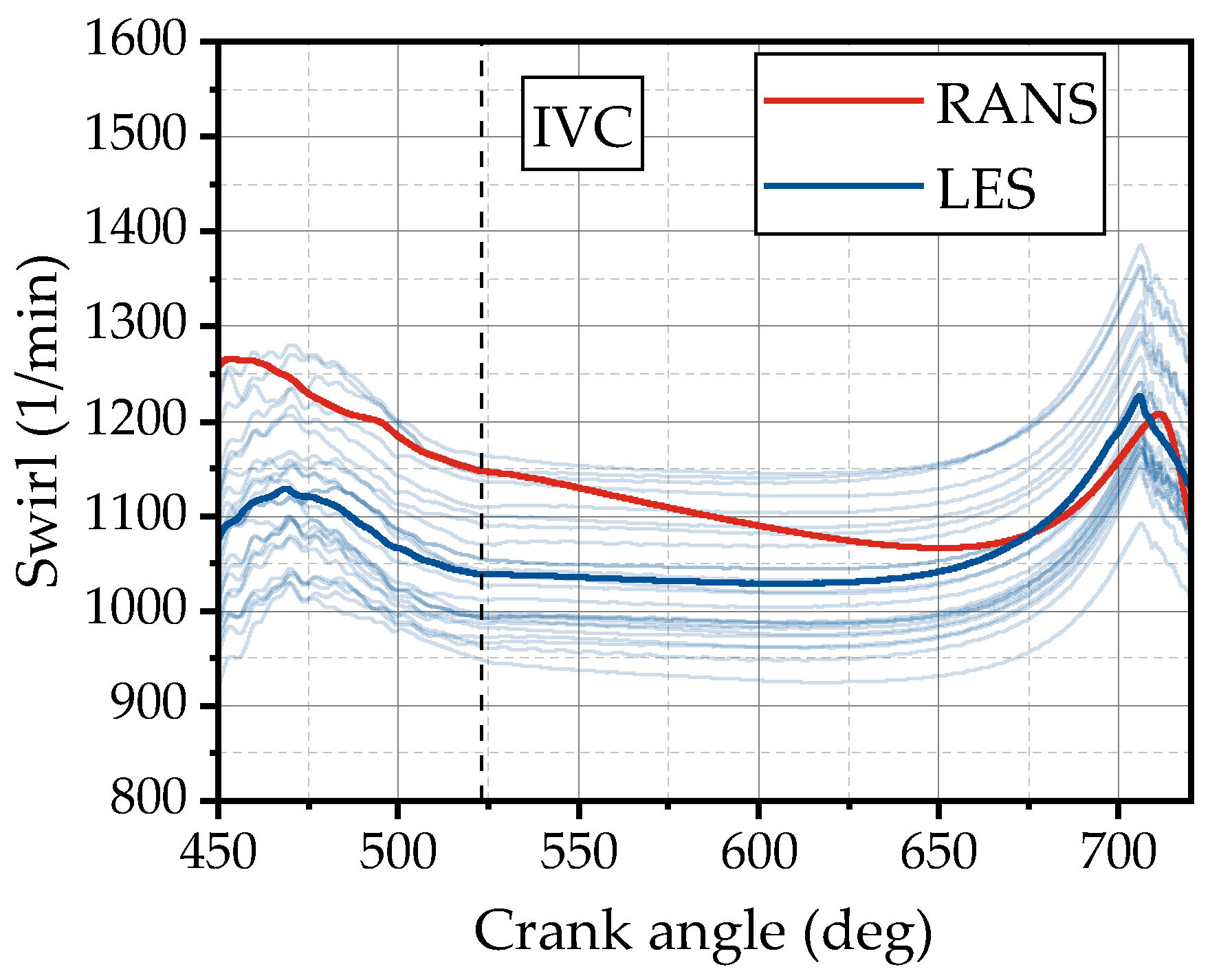
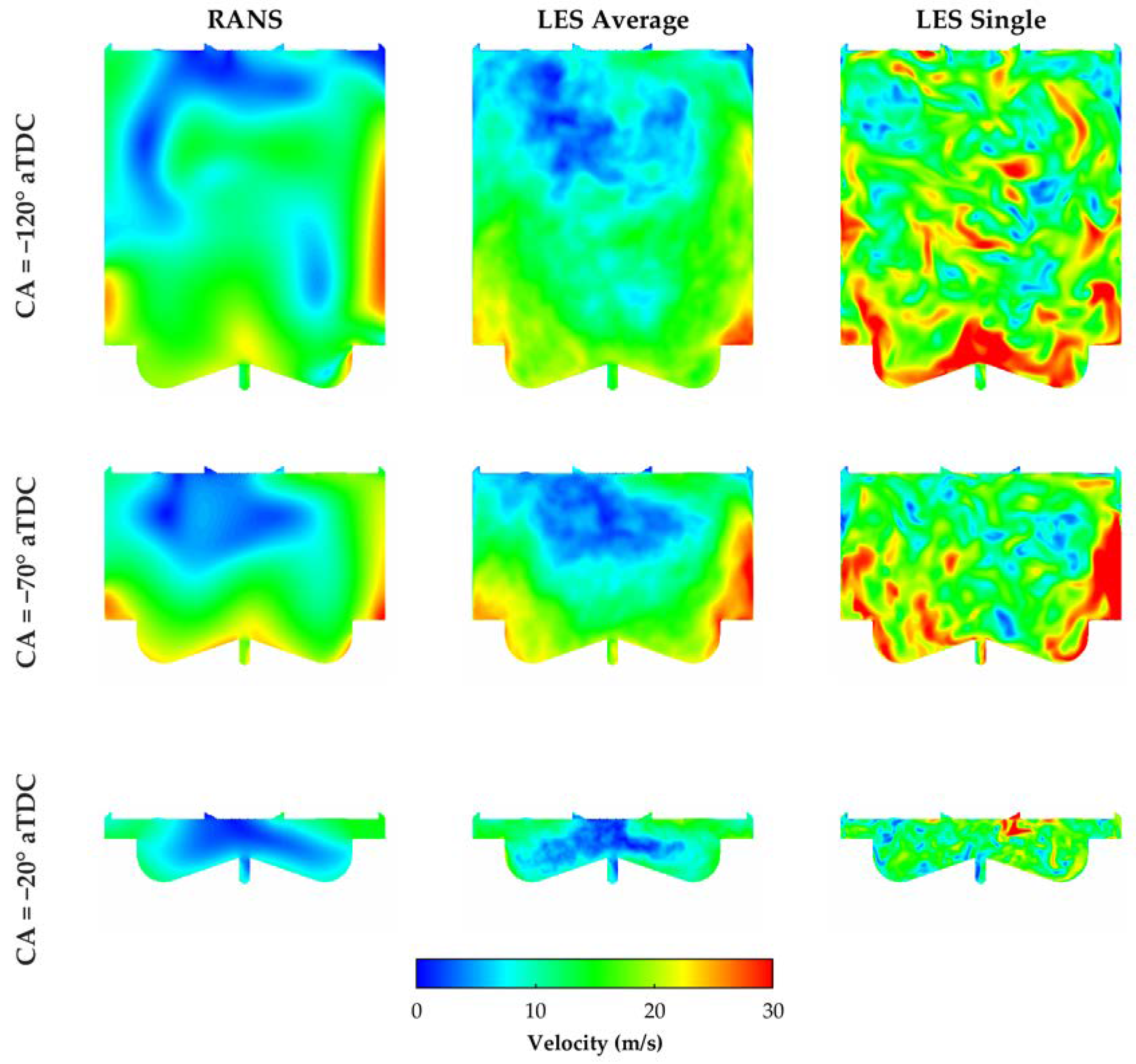
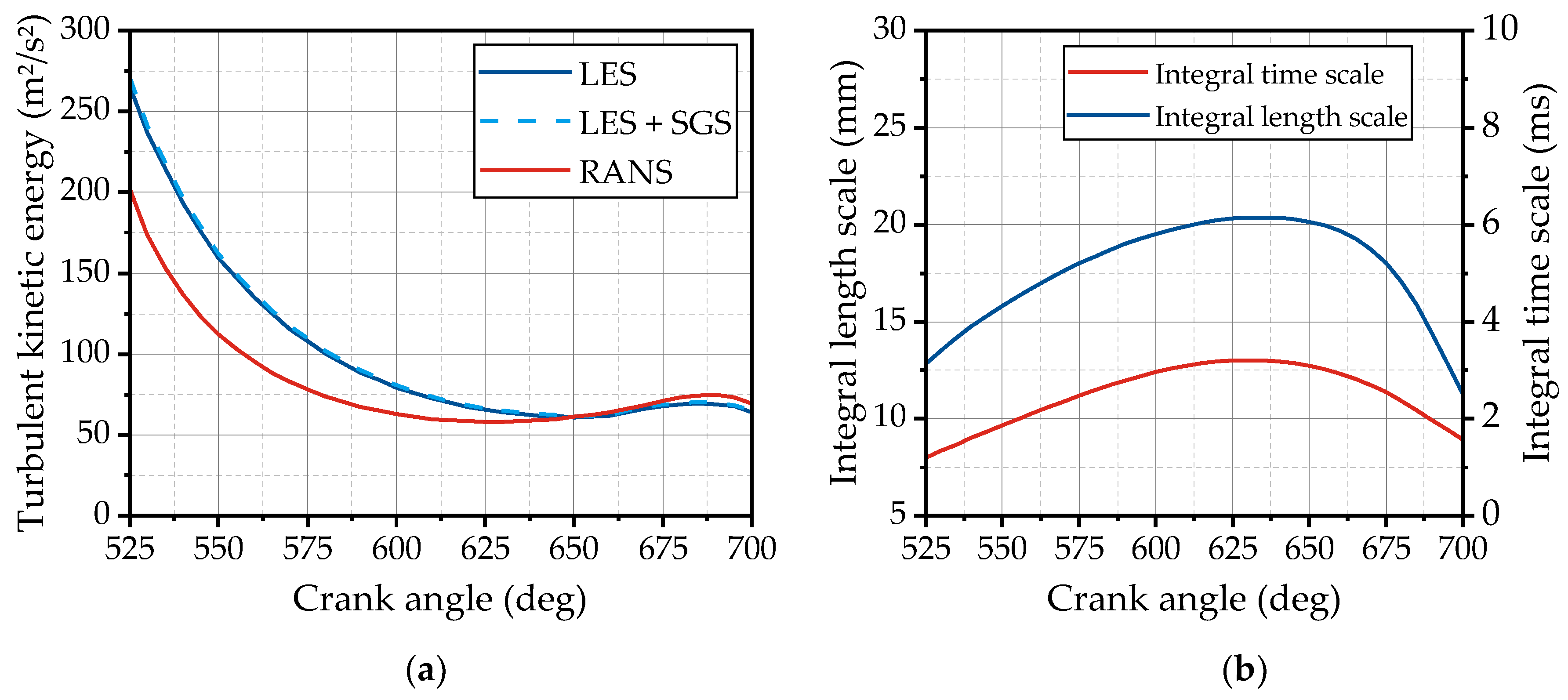
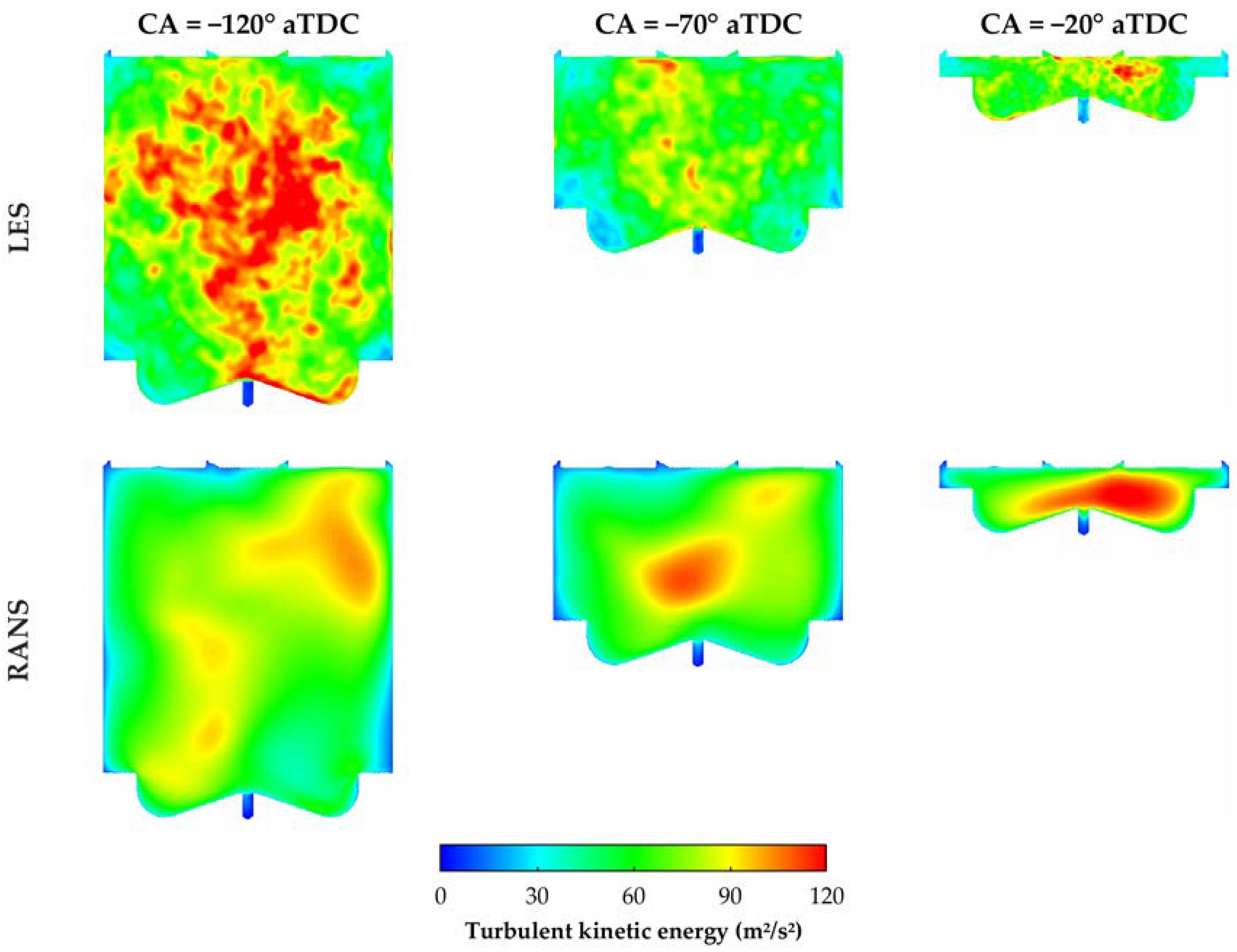
3.2. Evaluation of the Flow Field

In this subsection, the in-cylinder flow field is investigated. For this purpose, a RANS simulation is utilized and compared with the cycle-averaged results of the LES multicycle calculations. A detailed validation of the simulated flow field would raise the need for experimental data from an optically accessible engine test rig, which was not available in the present study. Following this, the flow field could only be investigated utilizing simulations. An important value to quantify the in-cylinder flow in the case of compression-ignition engines is the swirl intensity. The swirl within the cylinder was evaluated for every LES cycle and the RANS solution. Figure 5 depicts the resulting course of the swirl during the compression stroke. For an engine speed of 1800 rpm, the resulting swirl number is in the range of 0.5 to 0.75, which is quite low compared to conventional CI engines.
The single LES cycles show a high variation in the swirl level in the range of 950–1150 1/min, while the swirl stays constant for a long period during compression after the intake valves are closed. When approaching TDC, the swirl level increases due to an amplification effect of the squish flow, which is mainly a result of the design of the piston bowl. The RANS simulation instead does not show a period of constant swirl level. At IVC, a high swirl is present for the RANS simulation, which is located at the upper bound of the scatter band of the LES simulations. Compared with the mean value of the LES cycles, marked as a thick line, the RANS simulation predicts a higher swirl of about 100 1/min. However, the swirl level decreases during the compression to a level similar to the LES close to TDC, due to a higher dissipation characteristic for RANS.
In addition to the swirl level, the detailed velocity distribution in the cylinder is evaluated for a single LES cycle and the ensemble-averaged values derived from all 25 cycles. The resulting distributions are compared to the RANS solution at three different positions during compression in Figure 6. Thereby, the effect of the ensemble averaging becomes obvious when comparing the single LES cycle with the averaged flow field. The averaged LES field is overall in good agreement with the RANS results. This can be attributed to the fact that the RANS solution always depicts the average flow field.
In contrast, the LES depicts the instantaneous flow field of an individual cycle and so a sufficient number of cycles is needed to derive the average flow field. In terms of the mean flow quantities, a number of 10 cycles could already provide reasonable results, while a higher amount of about 25 cycles is needed to derive the RMS quantities with sufficient accuracy [42]. To minimize statistical inaccuracies, a number of 25 cycles is proposed to predict the mean quantities and a number of 50 cycles is recommended for the prediction of CCVs in [24]. However, the 25 cycles calculated in this study depict a compromise between accuracy and computational effort.
Furthermore, the turbulent kinetic energy is a decisive parameter when it comes to combustion. A higher level of turbulence promotes the mixture preparation of the pilot fuel and the flame speed in the premixed gas–air mixture. The traces of the in-cylinder turbulent kinetic energy (TKE) during compression are illustrated in Figure 7a for RANS and LES. While the TKE is in the case of RANS directly delivered by the turbulence model, it is not straightforward to derive the TKE from the LES. An approach to extract the TKE from LES results calculates the TKE as a function of the mean RMS velocities derived from the ensemble averaging proposed in [23,43]. This methodology was also chosen for evaluating the TKE due to its feasibility in terms of computational effort. However, it depicts a simplification as it partially allocates the CCVs of the mean flow to the TKE [41]. An overview of more detailed methods to derive the TKE from velocity data is given in [44].
In the case of LES, the TKE is additionally depicted including the subgrid-scale turbulence (SGS). Comparing this curve to the one without subgrid-scale turbulence illustrates the high amount of resolved turbulence, which is significantly over 90%. Following the chosen mesh resolution seems to be fine enough to fulfill the criterion proposed by Pope.
Shortly after the intake valves are closed at 525 °CA, the LES shows a higher value for the TKE than the RANS. This behavior was also observed in [43] and may result from an inadequate prediction of the turbulence generated by the flow through the intake valves and the shear flow generated by the inflow of the RANS. Furthermore, the RANS is limited due to the fact that it assumes isotropic turbulence, while the LES resolves the bigger turbulent eddies and captures the anisotropy of these complex flow structures. The TKE decreases during compression for both RANS and LES, while it starts to increase again when the piston approaches TDC due to turbulence generation by the squish flow. The values of the TKE are in good agreement between RANS and LES, starting from a crank angle of 630° until the start of injection at a crank angle of 700°.
In addition to the TKE, the integral length and time scales in the cylinder were evaluated based on the RANS solution and are depicted in Figure 7b during compression. The integral length depicts the size of the turbulent eddies, which are mainly responsible for turbulence production. During the intake airflow, the integral length scale can be related to the local thickness of the air jet entering the cylinder [41]. After the closing of the intake valves on the left edge in Figure 7b, the integral length shows a value of 12.8 mm, which is in the area of the maximum valve lift that is a decisive parameter for the air jet thickness. The integral length reaches its maximum in the middle of the compression stroke at 630 °CA and then rapidly decreases when the piston approaches TDC. Heywood [41] proposed estimating the integral length around TDC as 0.22 times the clearance height. The clearance height for the present engine at the start of injection at 700 °CA is 40 mm and can be defined as the highest distance from the piston bowl to the cylinder head. The length scale results in 8.8 mm, which is in the area of the calculated value of 11.3 mm derived from the RANS.
The distribution of the TKE in the cylinder is depicted in Figure 8 for three different crank angles for RANS and LES. On the left side, after a third of the compression stroke, the overall TKE predicted by the LES is still higher than the TKE derived from the RANS (see Figure 7a), which can be observed by a wider area captured by high TKE values. From a qualitative perspective, the agreement between RANS and LES increases in the second half of the compression stroke. However, there are still higher differences than for the mean velocity fields. This may be a result of the simplified turbulence treatment of the RANS, as already mentioned. In this case, LES provides an improvement of turbulence description and depicts an interesting alternative for future applications in the field of in-cylinder CFD.

4. Results

This section covers the detailed investigation of the combustion process conducted based on the results discussed in Section 3. At first, the heat release characteristics in terms of dual fuel are investigated, followed by a detailed analysis of the physics of the turbulent flame front. Finally, possible reasons for the occurrence of CCVs are ascertained.

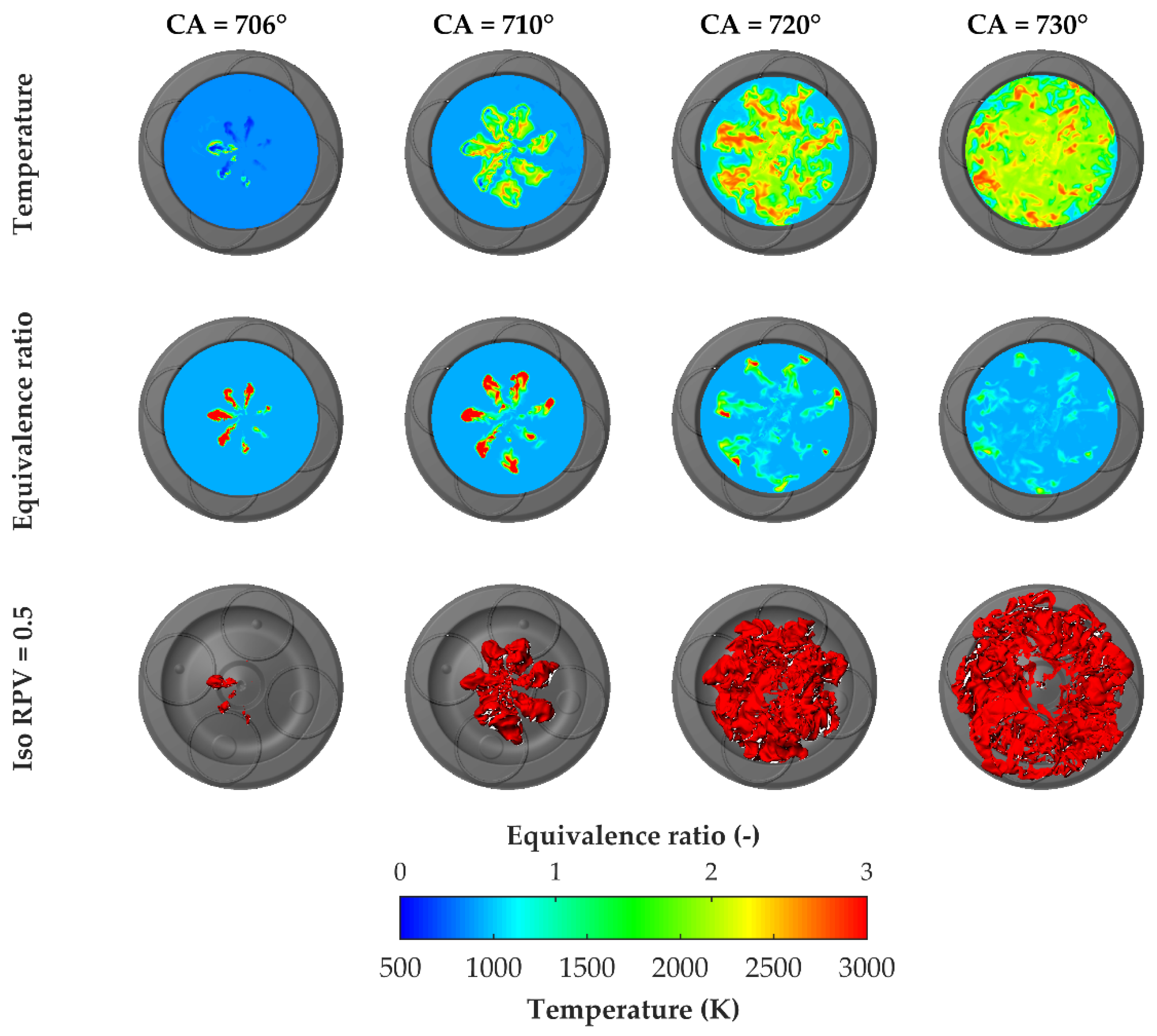
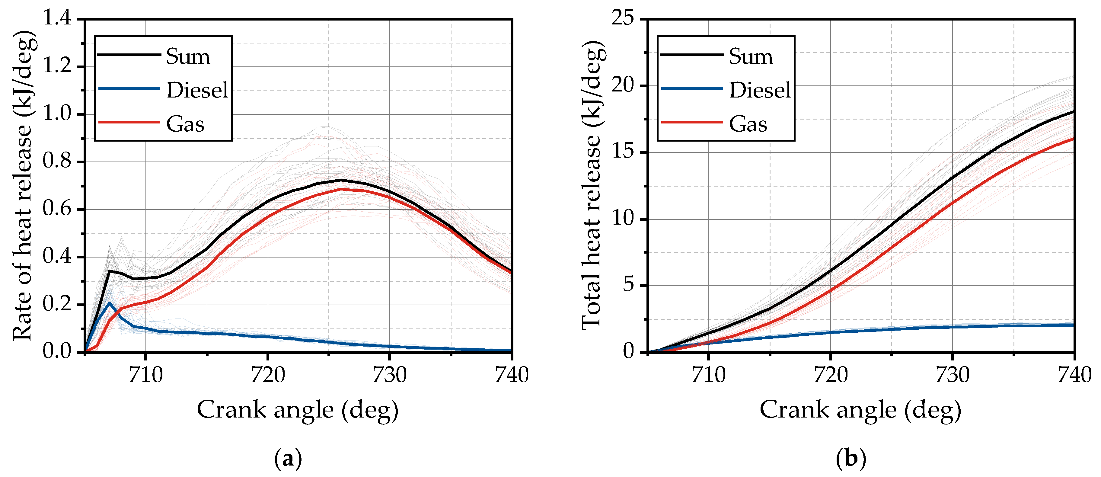
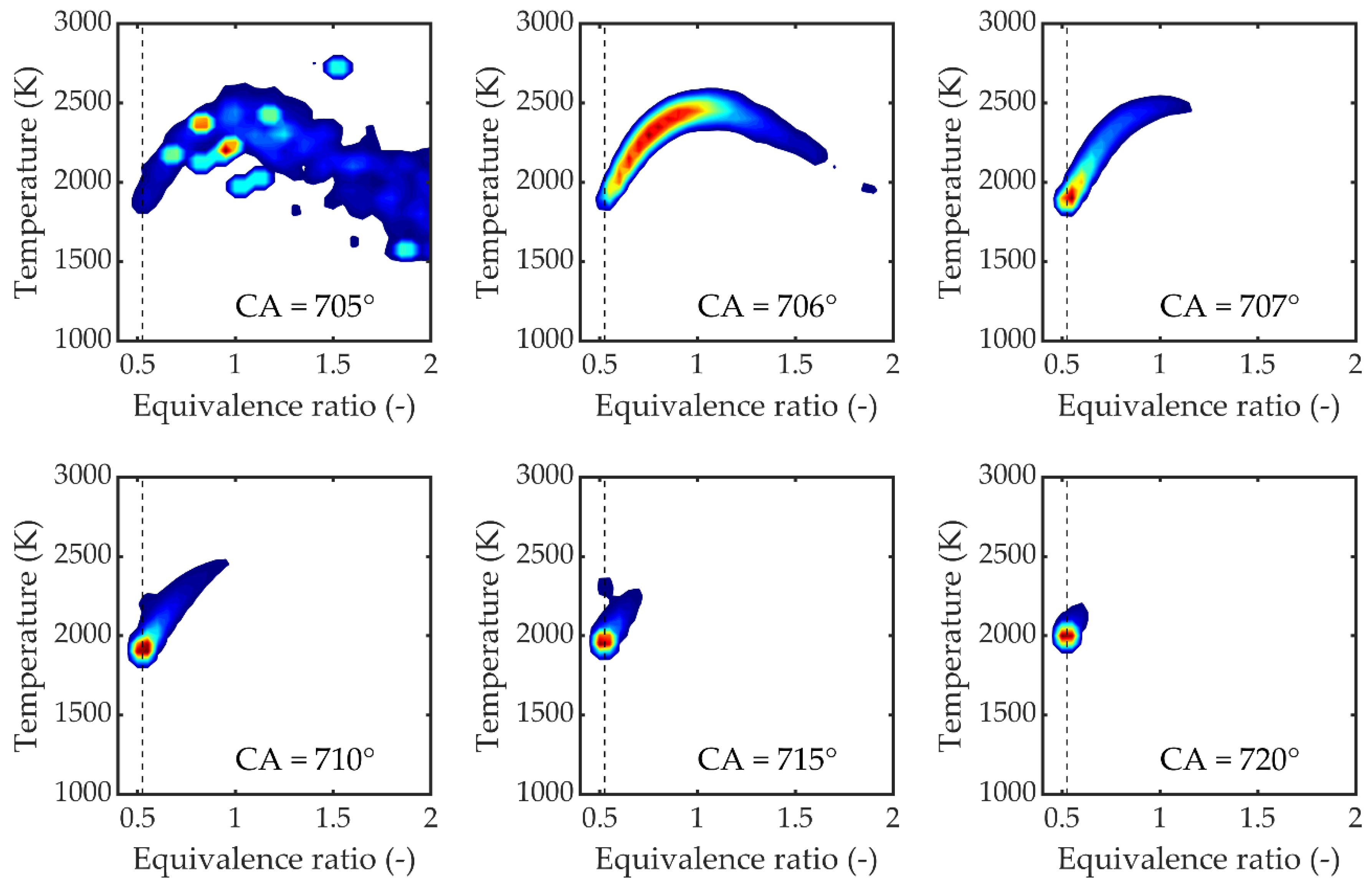
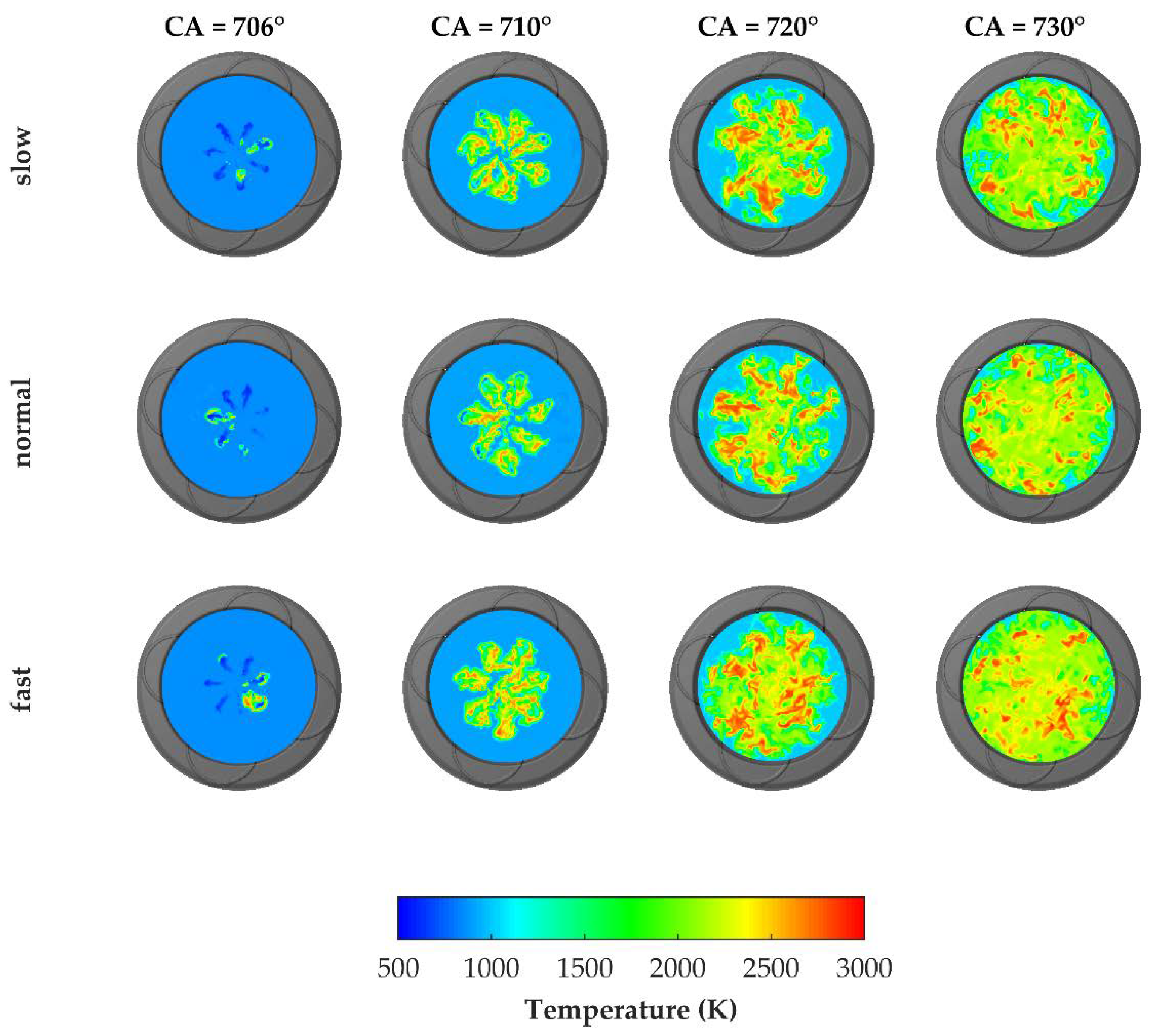
4.1. Dual Fuel Combustion

DF combustion constitutes, as already mentioned, a complex process that covers a wide range of combustion regimes. Figure 9 illustrates the distribution of temperature, equivalence ratio and the reaction progress variable (RPV) for three different crank angles around TDC to gain a deeper insight into the course of combustion. The RPV is defined as the ratio of the current combustion products and the theoretical maximum combustion products for a given fuel–air mixture. Temperature and equivalence ratio are evaluated on a conical surface located in the center axis of the spray plumes. The RPV is depicted as an isosurface with a value of 0.5 corresponding to the location of the flame front.
The ignition of the pilot fuel occurs at 706 °CA, indicated by temperature spots with more than 1500 K at three of the seven spray plumes. These plumes are located in the lower-left area and show wide regions of high equivalence ratio. On the right side of the piston bowl, the equivalence ratio is lower, which may be a hint to a higher interaction of the spray with the turbulent flow field, leading to a faster dilution of the ignition precursors and following a longer ignition delay. At 710 °CA, all spray plumes are burning, while there are still gaps between the plumes recognizable, indicating that no coherent flame front has yet formed. This changes at 720 °CA (TDC), where no distinct burning plumes can be spotted and the structure rather resembles a coherent flame front. At 730 °CA, almost the whole piston bowl is captured by the flame and it starts to enter the squish area indicated by the isosurface of the RPV.
During the combustion, a decisive process is the transition from the conversion of the pilot fuel to the premixed combustion of the lean natural gas–air mixture. The investigation of this process requires an analysis of the share of diesel and gas in the heat release given in Figure 10a for the rate of heat release and in Figure 10b for the total heat release. Thereby, the single LES cycles and the ensemble-averaged values (thick lines) are plotted. It is crucial to note that the heat release in Figure 10a,b is derived from the combustion model and can therefore not be directly compared to the heat release derived from the pressure traces in Figure 3b.
At the start of combustion, the rate of heat release shows a rapid rise caused by the instantaneous conversion of the ignitable pilot fuel that mixed up with the gas–air mixture during the ignition delay time. The blue diesel curve includes the natural gas entrained into the spray plume since the combustion model only utilizes one fuel component. Thus, the distinction between diesel and gas combustion can only be made by means of the equivalence ratio in the computational cells, whereby the limit was set to 0.6. This value was chosen because it represents an equivalence ratio slightly above the equivalence ratio of the background mixture. Higher equivalence ratios are only present in the spray area, where the diesel combustion occurs. One has to consider that based on this methodology, the heat release of the diesel combustion is calculated as a little too high due to the entrained natural gas that is attributed to it. The amount of entrained gas depends mainly on the injection properties and the gas concentration in the background mixture [45]. The red curve representing the lean gas combustion rapidly rises about 1 °CA after the blue diesel curve and reaches the same level of 0.2 kJ/deg as the diesel curve. This indicates that a significant amount of the lean natural gas–air mixture in the vicinity of the spray plumes is burnt and contributes almost half of the first peak of the sum curve. After the first peak, the heat release of the pilot fuel shows a persistent decline but still significantly contributes to the sum of the heat release. This phase can be characterized as diffusive combustion of the diesel fuel inside the spray plume. The gradient of the gas combustion shows a slight decrease after the first peak but then rises again rapidly. This behavior can be related to the conversion of the natural gas between the spray plumes and the formation of a coherent flame structure that rapidly expands, driven by turbulence, which can be seen in the transition from 710 °CA to 720 °CA in Figure 10. The heat release reaches its maximum at about 726 °CA and after that decreases due to a wide area of the combustion chamber being already captured by the flame and the beginning of the expansion. The observed phenomena during combustion are in good agreement with the experimental findings in [46].
In addition to the subdivision of the heat release conducted in Figure 10, the volume-based probability distribution of the temperature and the equivalence ratio, illustrated in Figure 11 for six different crank angles, can be investigated to gain a deeper insight into the combustion process. Thereby, the area at the back edge of the flame was evaluated based on the RPV limited by 0.9 and 0.95. This methodology was chosen to capture the maximum temperature that occurs in this area due to the fact that a large portion of the fuel is already converted in this area.
The values shown in Figure 11 represent the ensemble average of the LES cycles, whereby the evaluation of every single cycle was conducted before the averaging of the data. Thereby, the red color corresponds to a high probability of this regime in the evaluated area. At the point of ignition at 705 °CA, a wide area concerning the equivalence ratio is burning, including very rich areas in the pilot spray. Afterward, these areas are further mixed with air, leading to a shift in the regions of stoichiometric combustion at 706 °CA and 707 °CA. At 707 °CA, a significant proportion of heat is released in the area of the lean gas–air mixture, which is illustrated by the dashed line at an equivalence ratio of 0.55. This is further intensified in the following progress of combustion depicted at 710° CA and 715 °CA. Here, the share of heat release due to conversion of richer areas diminishes in importance, as already depicted in Figure 10. At 720 °CA (TDC), there is only a small area corresponding to richer combustion in the area of equivalence ratios higher than 0.55 recognizable. The observed distribution of temperature during combustion is the main reason for the lower formation of nitrogen oxides in the case of DF combustion, since high temperatures that promote the formation of nitrogen oxides only occur within a short time frame. Since the formation of nitrogen oxides is not the focus of this study, it is not discussed further.

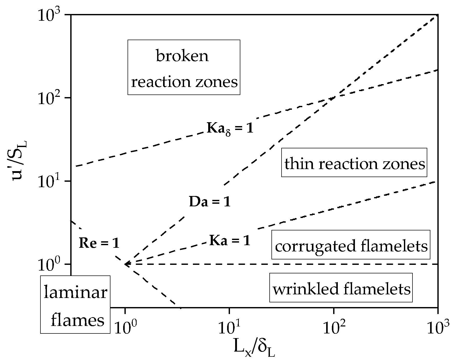
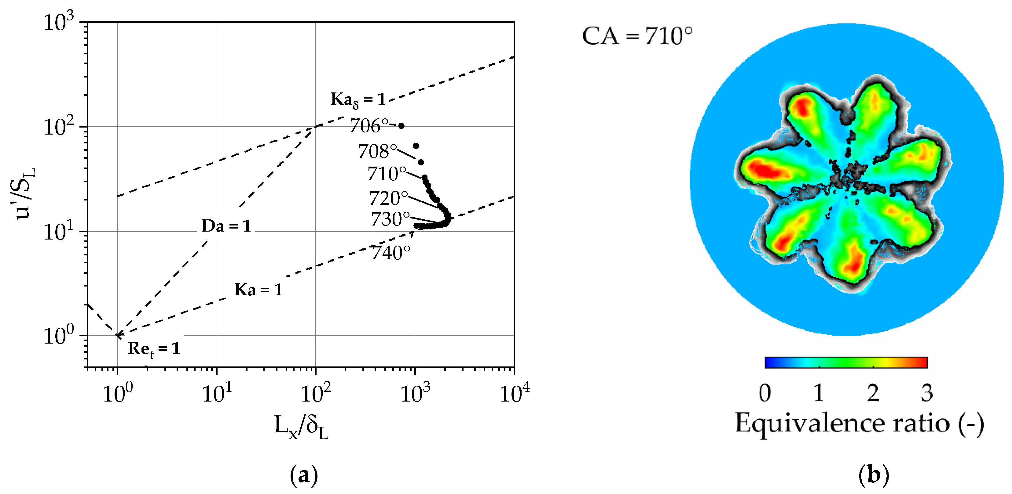
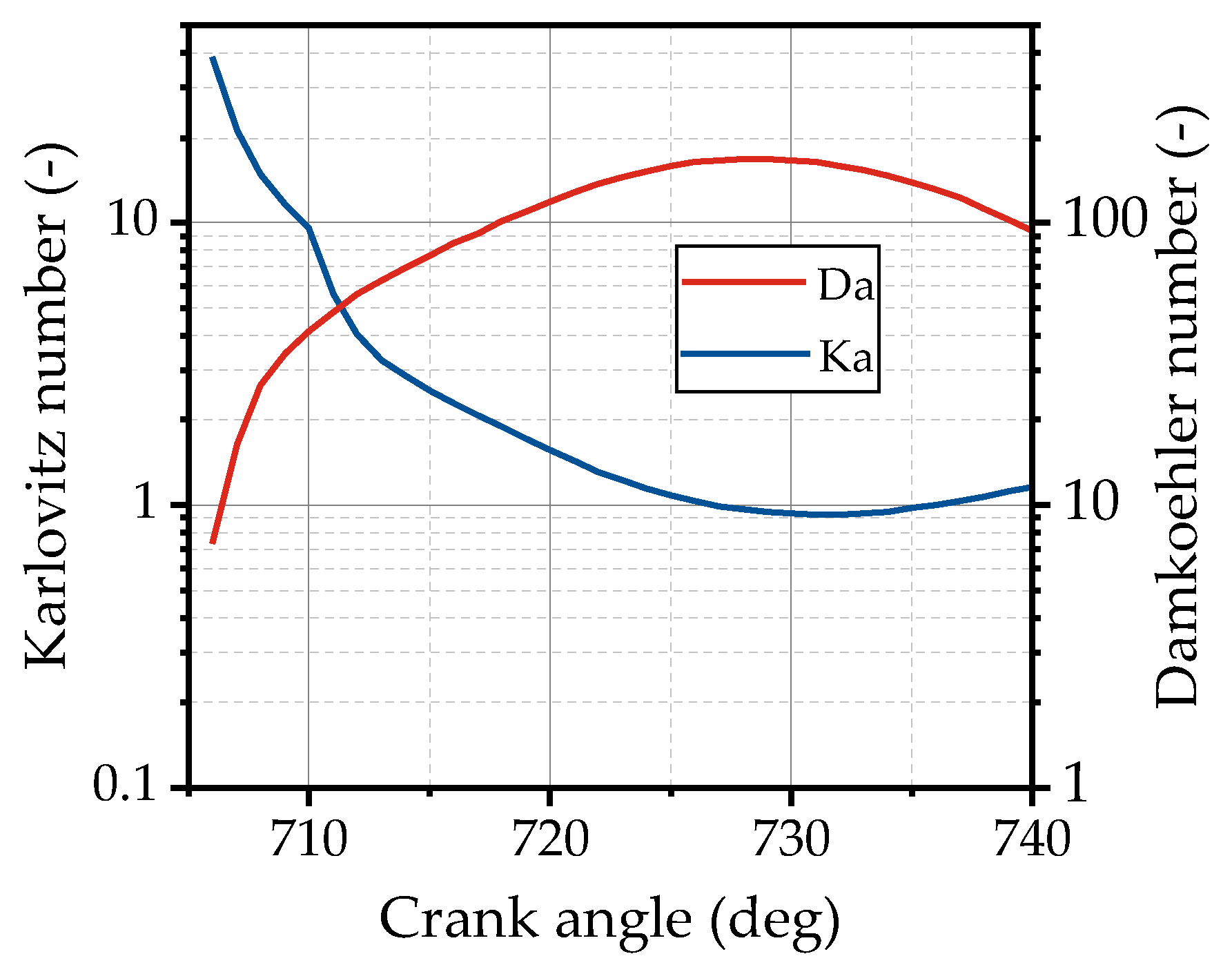
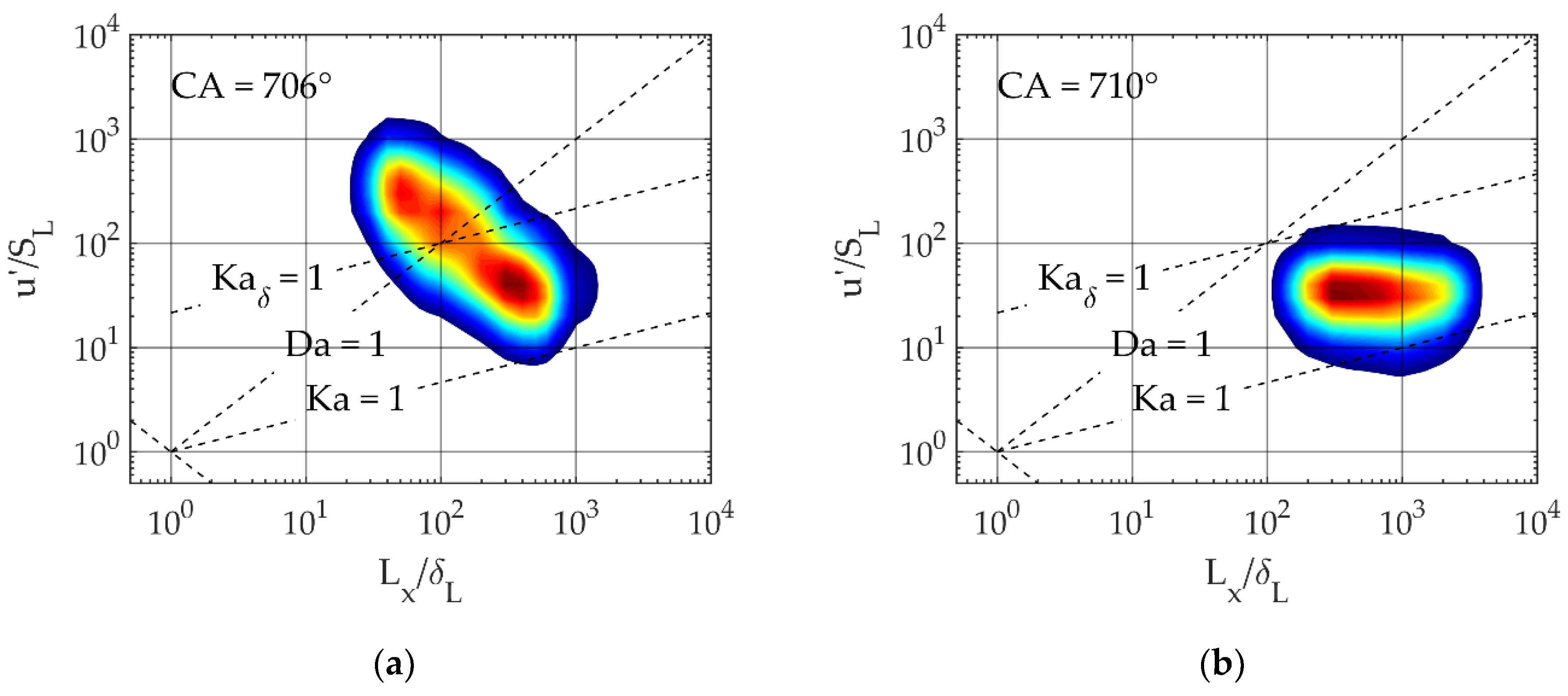
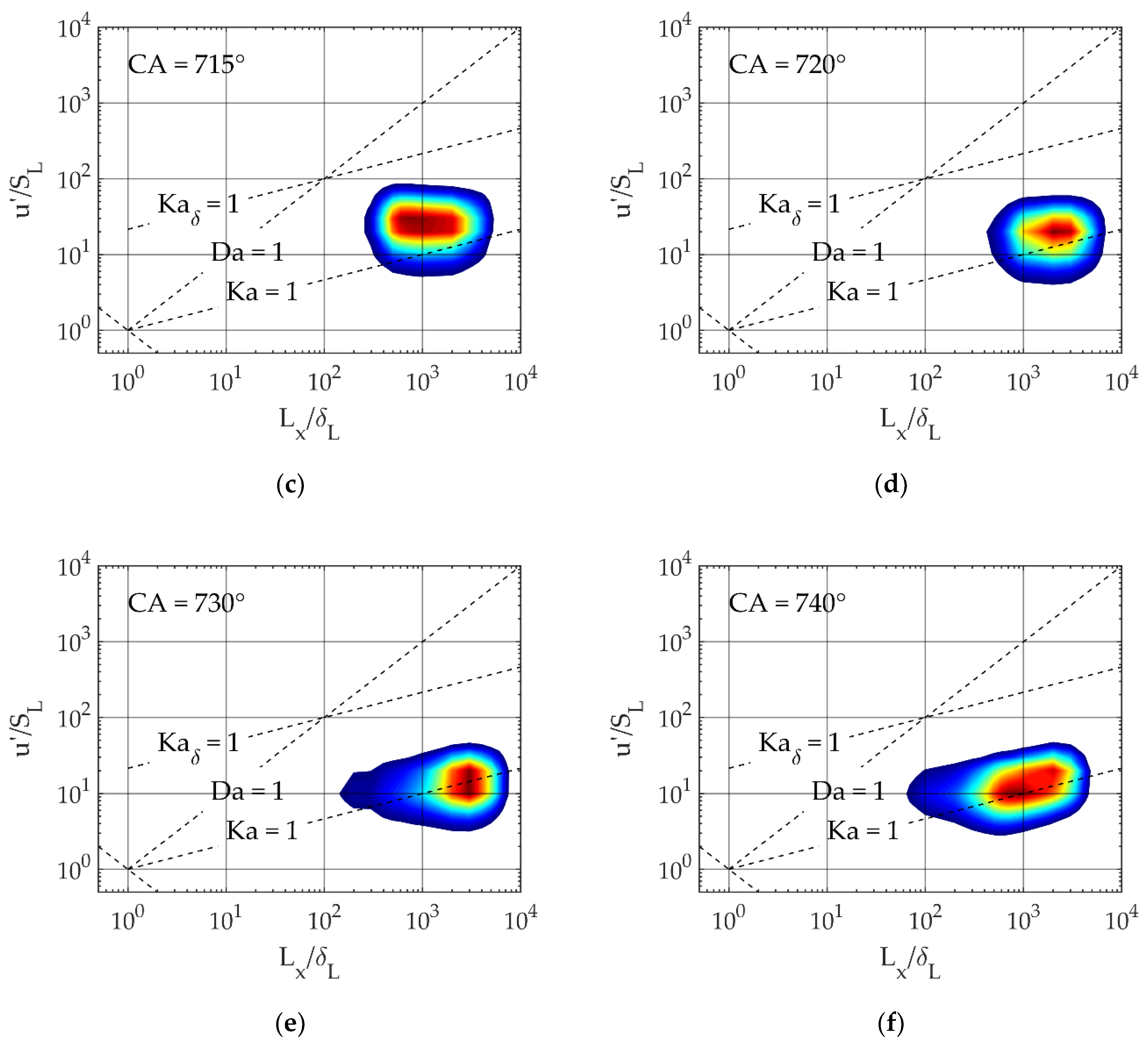
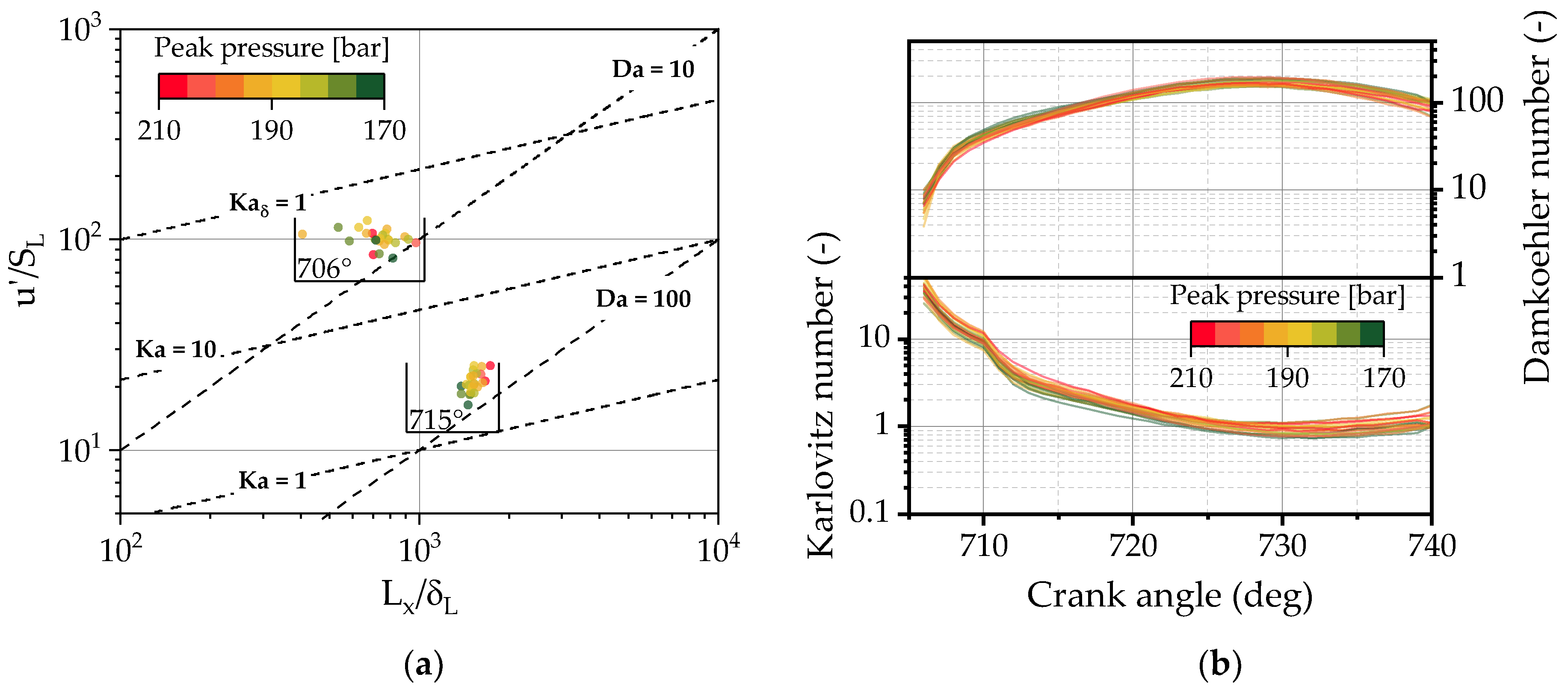
4.2. Analysis of Combustion Regimes

In this section, the characteristics of the turbulent flame are investigated in detail to gain a deeper insight into the phenomenology of DF combustion. An important tool for this purpose is the regime diagram proposed by Peters [47], which classifies the interactions of the turbulent flow and the flame front into different regimes depending on the ratio of the turbulent fluctuation intensity u’ to the laminar flame speed SL and the ratio of the turbulent length scale Lx to the laminar flame front thickness δL. The different regimes are shown in the so-called Borghi–Peters diagram in Figure 12. In the bottom left corner, the laminar flames are separated from the turbulent flames by the dashed line representing a Reynolds number of 1 according to Equation (7). The turbulent flame regime can be subdivided by means of the Damkoehler number (Da) and the Karlovitz number (Ka) defined by Equations (8) and (9). The Damkoehler number indicates the influence of the turbulent flow on the ongoing chemical processes inside the flame and is defined as the ratio of the turbulent time scales τT and the time scales of the flame τL. In addition, the Karlovitz number is a measure for the interaction of flame with the smallest scales of turbulence, the Kolmogorov scales. It is defined as the ratio of flame time to Kolmogorov time τK.
R e = u L x S L δ L
D a = τ T τ L = S L L x u δ L
K a = τ L τ K = δ L 2 η ²  
The dashed line represented by a Karlovitz number of one separates the corrugated flamelets, where the smallest eddies cannot enter the flame, from the regime of thin reaction zones. For Ka > 1, the smallest eddies enter the flame, which leads to a perturbation of the flame and influences scalar and temperature gradients. However, in the regime of thin reaction zones, the smallest eddies cannot penetrate into the reaction zone and do not influence the chemical processes. Peters [47] introduced a second Karlovitz number, Kaδ, where the laminar flame thickness in Equation (9) is replaced by the thickness of the reaction zone, which is usually in the range of one-tenth of the flame thickness. Kaδ = 1 functions as an upper bound for the regime of thin reaction zones. Above this limit, the eddies enter the reaction zone and affect the chemical reactions in the regime of broken reaction zones.
A methodology to extract the combustion regimes from the LES results was developed based on the evaluation of the area in the vicinity of the flame front. This area is specified by the reaction progress variable in the range of 0.1 to 0.5. The properties needed for the Borghi–Peters plot were extracted for every cycle and their ensemble average was used to calculate a mean value for the evaluated area. The integral length was taken from the RANS solution, which depicts a simplification since it is not straightforward to calculate the integral length from the LES. The results are shown in Figure 13a for different crank angles during combustion. To clarify the methodology, an example of the evaluated area is illustrated in Figure 13b as isolines starting from 0.1, represented by the white line, to 0.5, represented by the black line. The lines are shown on a conical surface of the equivalence ratio through the spray plumes at 710 °CA. At the beginning of the combustion at 706 °CA, the flame is situated close to Kaδ = 1. This is mainly a result of a high turbulence level generated by the pilot injection. After the start of combustion, the flame rapidly moves downwards in the regime diagram due to a transition into the lean gas combustion, driven by the turbulence of the in-cylinder flow.
From about 715 °CA to 740 °CA, the shape is similar to the shape observed by Linse et al. [48] in terms of gasoline engines. From a quantitative point of view, the results in the case of DF combustion are shifted to the upper right compared to gasoline combustion. This is mainly the result of an increased turbulence level and a higher in-cylinder pressure during combustion that reduces the laminar flame thickness. From 725 °CA on, the flame is close to the limit of the corrugated flamelet regime represented by Ka = 1. The course of DF combustion covers a wide area of the thin reaction zone’s regime and therefore has to deal with a strongly varying interaction of the turbulent eddies and the flame.
The width of the covered interactions becomes obvious when evaluating the Damkoehler and Karlovitz number during combustion, as illustrated in Figure 14. The Damkoehler number increases by an order of magnitude, clarifying the increasing importance of turbulence on flame propagation. This effect is attributed to the transition from the rapid conversion of the pilot fuel to turbulence-driven gas combustion. In addition, the Karlovitz number decreases by an order of magnitude, indicating a waning influence of the small scales of turbulence on the flame front, which is mainly an effect of the decreasing flame thickness due to a higher cylinder pressure close to TDC.
A more detailed investigation of the flame is given in Figure 15, whereby the volume-based probability of the occurrence of the different regimes inside the flame is depicted as surface for six different crank angles. At 706 °CA, a wide area of the thin reaction zone’s regime and a significant part of the broken reaction zone’s regime are covered. Inside the broken reaction zone’s regime, the smallest eddies enter the inner reaction zone of the flame and affect the ongoing chemical reactions. This indicates that turbulence–chemistry interaction (TCI) significantly contributes to the ignition and the conversion of the pilot fuel, while it becomes less important during lean gas combustion. Following these findings, integrating a TCI model may improve the simulation results in the first part of combustion. At 710 °CA, the flame covers a large part of the thin reaction zone’s regime, demonstrating that the transition from the conversion of the pilot fuel to the lean gas combustion is already hardly affected by TCI. Afterward, the surface moves downwards in the regime diagram until a significant share of the flame reaches the regime of corrugated flamelets. Thus, a substantial part of the flame is not affected by entering the smallest eddies into the flame front. In this region, the turbulent flame speed is mainly dependent on the surface increase through the interaction of the flame front with the turbulent flow structures. The findings in this subsection illustrate the complexity of the turbulent flame and deliver detailed information with regard to the phenomena that are necessary to capture by the development of future combustion models in terms of DF combustion.

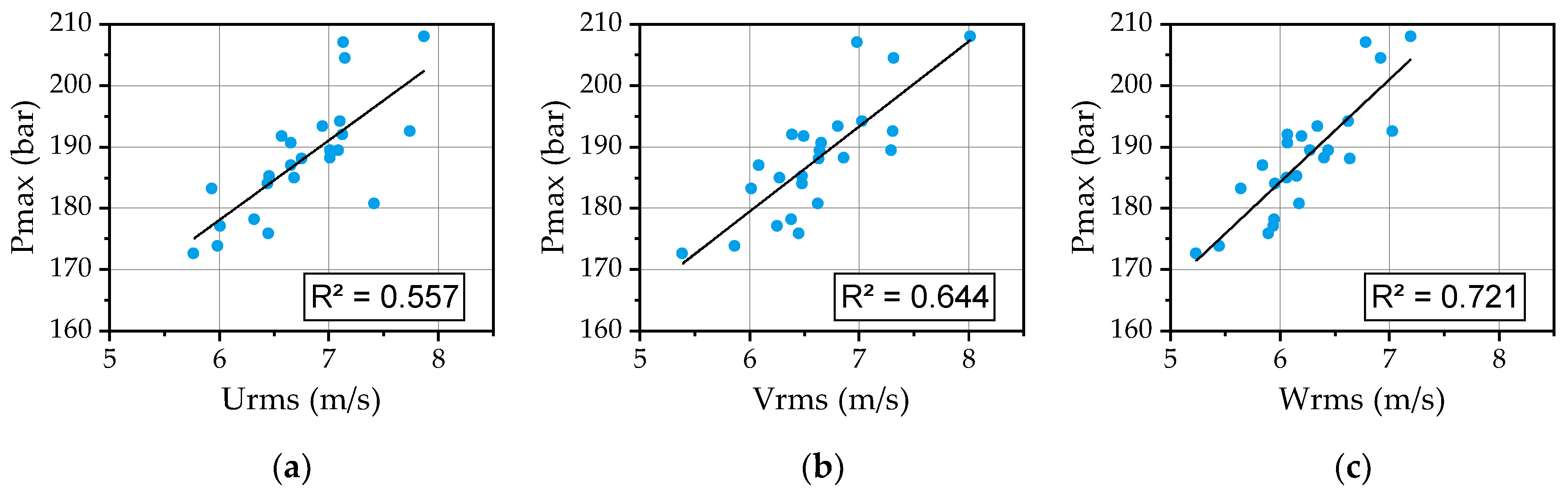
4.3. Cycle-to-Cycle Variations

In this subsection, the occurrence of CCVs and their possible origins are addressed in detail. CCVs depict an important factor in ensuring stable engine operation and should be kept as low as possible. There are many different reasons for the occurrence of CCVs in terms of DF combustion that the present study in its entirety cannot investigate. The focus here was on the impact of the turbulent fluctuations of the in-cylinder flow on flame propagation. As mentioned in [7], the pilot injection is also a possible source of CCVs due to strong varying conditions at the nozzle exit. However, this was not considered in the present study.
A crucial factor for CCVs is the interaction of the turbulence with the pilot spray and the flame front. The influence of the turbulence on the peak pressure and thus the combustion speed can be clarified by evaluating the RMS velocities of the in-cylinder flow in the three spatial directions. Figure 16a illustrates the peak pressure’s dependence on the RMS velocity in the x-direction Urms. A certain correlation between the increase in the RMS velocity and the peak pressure can be found. This correlation becomes more obvious in Figure 16b, where the RMS velocity in y-direction Vrms is evaluated. A distinct correlation is present in terms of the RMS velocity in z-direction Wrms depicted in Figure 16c. This observation may result from the turbulence generated by the fluctuations of the squish flow, which enhances scalar transport and flame propagation in the piston bowl. However, an adequate assessment of this effect needs further investigations of the spatial intensity distribution of the turbulent fluctuations.
The ignition and flame propagation for different fast-burning cycles can be visualized using the temperature distribution in the piston bowl depicted as a conical surface through the spray plumes in Figure 17. Thereby, three different cycles are illustrated at four different crank angles around TDC. At the start of combustion at 706 °CA, the fastest cycle in the bottom row shows the largest area initially captured by the flame, although only three of the seven spray plumes are already burning. The first ignited spray plumes vary from cycle to cycle and depend on the interaction with the local flow structures. Moving on to 710 °CA, the transition into the gas combustion begins. Thereby, the area between the spray plumes mainly containing a lean natural gas–air mixture starts to burn in the fast-burning cycle, while this cannot be observed for the slow-burning cycle. For the intermediate burning cycle in the middle row, there is only one burning gap recognizable. This phenomenon results in an earlier formation of a flame front that propagates through the lean gas–air mixture and enhances heat release. The origin of the higher heat release clarifies at 720 °CA, where the flame captures almost the whole piston bowl in the fast-burning case. At 730 °CA, this is the case for all cycles and the flame starts to pass into the squish area, which cannot be seen in this illustration due to the position of the conical surface. Finally, the phenomenon of the flame initiation inside the lean gas–air mixture between the spray plumes can be identified as one trigger for fast-burning cycles.
The CCVs can also be addressed by employing the Borghi–Peters diagram, as depicted in Figure 18a. Thereby, the mean values of the evaluated area described in Figure 13b are depicted for the single LES cycle as a function of the corresponding peak pressure for two different crank angles.
The first point at 706 °CA represents the start of combustion and the second point at 715 °CA depicts the angle at which the lean gas combustion is already dominant concerning the rate of heat release. At 706 °CA, there is no recognizable correlation between the combustion regimes and the peak pressure of the corresponding cycle. This changes with increasing gas combustion at 715 °CA, where a distinct correlation between the combustion regime and the peak pressure is recognizable. A higher peak pressure can be related to a higher interaction of the turbulent structures with the flame in terms of enhancement of scalar transport inside the flame front and wrinkling of the flame front. This effect is also recognizable in Figure 18b, where the Damkoehler and Karlovitz number are plotted as a function of the peak pressure over crank angle. In the case of the Karlovitz number, a correlation with the peak pressure is present. The fast-burning cycles line up at the upper bound of the scatter band as soon as the gas combustion becomes dominant at 715 °CA. This results from an enhanced interaction of the turbulent structures with the flame front that speeds up scalar transport and increases the flame surface by wrinkling.

5. Conclusions

In the present work, an extended coherent flame model was adapted to consider the effect of a delayed ignition due to the presence of natural gas. This was conducted by optimizing the parameters of the Arrhenius function utilized for the calculation of the ignition delay, based on tabulated ignition delays derived from a dual fuel reaction mechanism. Based on this model and on a model to describe the pilot injection of the diesel fuel in the ballistic working regime developed in a previous study, 25 consecutive engine cycles were simulated employing LES. The model was validated against experimentally determined pressure traces derived from a single-cylinder engine test rig. Thereby, a good agreement of the pressure traces and the deduced rate of heat release could be achieved. Furthermore, cycle-to-cycle variations were predicted with sufficient accuracy, whereby a large share of the experimentally determined scatter band was captured.
The flow field derived from the LES was ensemble averaged and compared to a RANS solution during the compression stroke, whereby the mean flow quantities were in good agreement. In addition, the turbulence kinetic energy was calculated based on the velocity fluctuations around the ensemble average of the LES. Although this methodology represents a simplification, the results are reasonable and give an insight into the ability of LES to improve the prediction of turbulence. This is caused by a direct resolution of the flow structures containing over 90% of the turbulent kinetic energy. Even the flow around the intake valves and the shear flow in the area of the air jet inside the cylinder during the intake stroke can be captured by LES more suitably.
Furthermore, the dual fuel combustion process was investigated in detail by analyzing the contribution of regimes with different equivalence ratios to the rate of heat release. In the first few degrees of crank angle of combustion, the diesel fuel mixed with air is rapidly converted. Thereby, a significant amount of natural gas that was sucked into the spray plume and in the vicinity of the pilot spray was also burnt. It could be clarified that natural gas contributes almost half of the rate of heat release at this point. In addition, the transition into the premixed gas combustion could be spotted when the area between the spray plumes started to burn and formed a coherent flame front together with the burning spray tips.
A detailed analysis of the turbulent combustion regimes using the Borghi–Peters diagram showed that the dual fuel combustion covers a wide area of different combustion regimes. It mainly occurs in thin reaction zones, wherein the smallest eddies can enter the flame and enhance the scalar transport inside the flame front. At the point of ignition, there is also a significant share of the flame in the regimes of broken reaction zones detectable, where the smallest eddies enter the reaction zone. This leads to the conclusion that including turbulence–chemistry interaction in the modeling approach may improve the prediction of the ignition delay. During the flame propagation in the lean natural gas–air mixture, turbulence–chemistry interaction hardly matters.
Cycle-to-cycle variations were addressed and a distinct dependency of the peak pressure of a single-engine cycle on the velocity fluctuations in the direction of the cylinder axis could be found. This indicated that the turbulence of the squish flow might have a significant influence on cycle-to-cycle variations. Furthermore, the ignition of the natural gas between the spray plumes during the transition to the premixed gas combustion could be spotted as a trigger for cycle-to-cycle variations. Another factor is depicted by the intensity of the interaction with the turbulent flow field, whereby high Karlovitz numbers accompany high peak pressures.
Finally, the findings contribute to the understanding of the dual fuel combustion process and serve as a basis for the development of further combustion models. Thereby, the initialization of the flame surface density in terms of ECFMs and the transition into the premixed gas combustion are the most important points that should be addressed in the future from the authors’ point of view. However, due to the wide area of turbulent combustion regimes that have to be addressed by the modeling, this depicts a great challenge.

Author Contributions

Conceptualization, J.F. and T.L.; methodology, J.F. and T.L.; software, J.F.; validation, J.F; formal analysis, J.F.; investigation, J.F. and T.L.; resources, T.L.; data curation, J.F.; writing—original draft preparation, J.F.; writing—review and editing, J.F. and T.L.; visualization, J.F.; supervision, T.L.; funding acquisition, T.L. All authors have read and agreed to the published version of the manuscript.

Funding

This work was funded by Österreichische Forschungsförderungsgesellschaft in the framework of the BRIDGE project “DualFlame”, grant number 850690.

Institutional Review Board Statement

Not applicable.

Informed Consent Statement

Not applicable.

Data Availability Statement

All the data of the reported results can be found in the paper text.

Acknowledgments

The authors would like to thank the team of the Vienna Scientific Cluster (VSC) for providing the computational power for the multicycle simulations.

Conflicts of Interest

The authors declare no conflict of interest.

Abbreviations

The following abbreviations are used in this manuscript:
BDCBottom Dead Center
CACrank Angle
CCVCycle-to-Cycle Variation
CFDComputational Fluid Dynamics
COVCoefficient of Variation
LESLarge Eddy Simulation
DFDual Fuel
DIGEDiesel Ignited Gas Engine
ECAEmission Controlled Area
ECFMExtended Coherent Flame Model
IMOInternational Maritime Organization
IVCIntake Valve Close
MFBMass Fraction Burnt
RANSReynolds-Averaged Navier–Stokes
RPVReaction Progress Variable
RMSRoot Mean Square
SGSSubgrid-scale
TCITurbulence Chemistry Interaction
TDCTop Dead Center

Nomenclature

AArea
B0,1Wave model constants
CdDrag coefficient
DDestruction term
DaDamkoehler number
FDDrag force
Ka, KaδKarlovitz number
LxTurbulent length scale
PPressure
P1,2,3Production terms
rRadius
ReReynolds number
sFlame speed
ScSchmidt number
U, u, V, v, WVelocity
u’Turbulent fluctuation intensity
VVolume
xDistance
yMass fraction
δFlame thickness
ηKolmogorov length
ΛWave length
μViscosity
ρDensity
ΣFlame surface density
σStandard deviation
τTime scale
ΩGrowth rate
ωReaction rate

Subscripts

dDroplet
FFuel
gGas
iCoordinate direction (x, y, z)
KKolmogorov
LLaminar
lLiquid
pParent droplet
TTurbulent
uUnburnt

References

  1. International Maritime Organization. Resolution MEPC.176(58)—Revised MARPOL Annex VI; International Maritime Organization: London, UK, 2008; (MEPC.176(58)). [Google Scholar]
  2. Schlemmer-Kelling, U. Agenda 2030—mega trends in the large-bore marine engine business. In Proceedings of the Heavy-Duty-, On- and Off-Highway Engines Conference, Augsburg, Germany, 28–29 November 2017. [Google Scholar] [CrossRef]
  3. van Basshuysen, R. Natural Gas and Renewable Methane for Powertrains: Future Strategies for a Climate-Neutral Mobility, 1st ed.; Springer: Berlin/Heidelberg, Germany, 2016; ISBN 9783319232256. [Google Scholar]
  4. Karim, G.A. Dual-Fuel Diesel Engines; CRC Press: Boca Raton, FL, USA; London, UK; New York, NY, USA, 2015; ISBN 9781498703086. [Google Scholar]
  5. Baufeld, T.; Mohr, H.; Phillipp, H. Future Perspectives and technical Challenges for large-bore Dual-Fuel Engines. In Proceedings of the Dessau Gas Engine Conference, Dessau-Roßlau, Germany, 21–22 March 2013. [Google Scholar]
  6. Senghass, C.; Willmann, M.; Koch, H.-J. Simplified L’Orange fuel injection system for Dual Fuel applications. In Proceedings of the CIMAC Congress 2016, Helsinki, Finland, 6–9 June 2016. [Google Scholar]
  7. Königsson, F. On Combustion in the CNG-Diesel Dual Fuel Engine; Industrial Engineering and Management, KTH Royal Institute of Technology: Stockholm, Sweden, 2014; ISBN 978-91-7595-243-7. [Google Scholar]
  8. Frühhaber, J.; Peter, A.; Schuh, S.; Lauer, T.; Wensing, M.; Winter, F.; Priesching, P.; Pachler, K. Modeling the Pilot Injection and the Ignition Process of a Dual Fuel Injector with Experimental Data from a Combustion Chamber Using Detailed Reaction Kinetics. In SAE Technical Paper 2018-01-1724; SAE International: Warrendale, PA, USA, 2017. [Google Scholar] [CrossRef]
  9. Kahila, H.; Wehrfritz, A.; Kaario, O.; Vuorinen, V. Large-eddy simulation of dual-fuel ignition: Diesel spray injection into a lean methane-air mixture. Combust. Flame 2019, 199, 131–151. [Google Scholar] [CrossRef]
  10. Zhao, W.; Zhou, L.; Liu, Z.; Qi, J.; Lu, Z.; Wei, H.; Shu, G. Numerical Study on the Combustion Process of n-heptane Spray Flame in Methane Environment Using Large Eddy Simulation. Combust. Sci. Technol. 2021, 193, 142–166. [Google Scholar] [CrossRef]
  11. Demosthenous, E.; Borghesi, G.; Mastorakos, E.; Cant, R.S. Direct Numerical Simulations of premixed methane flame initiation by pilot n-heptane spray autoignition. Combust. Flame 2016, 163, 122–137. [Google Scholar] [CrossRef] [Green Version]
  12. Tekgül, B.; Kahila, H.; Kaario, O.; Vuorinen, V. Large-eddy simulation of dual-fuel spray ignition at different ambient temperatures. Combust. Flame 2020, 215, 51–65. [Google Scholar] [CrossRef]
  13. Ratzke, A.; Dinkelacker, F. Modellierung der Flammenausbreitung und des Flammenlöschens im Gasmotor; PZH-Verlag: Garbsen, Germany, 2013. [Google Scholar]
  14. Hockett, A.; Hampson, G.; Marchese, A.J. Development and Validation of a Reduced Chemical Kinetic Mechanism for Computational Fluid Dynamics Simulations of Natural Gas/Diesel Dual-Fuel Engines. Energy Fuels 2016, 30, 2414–2427. [Google Scholar] [CrossRef]
  15. Frankl, S.; Gleis, S.; Wachtmeister, G. Interpretation of Ignition and Combustion in a Full-Optical High-Pressure-Dual-Fuel (HPDF) Engine using 3D-CFD Methods. In Proceedings of the 29th CIMAC World Congress on Combustion Engine, Meeting the Future of Combustion Engines, Vancouver, BC, Canada, 10–14 June 2019. [Google Scholar]
  16. Li, Y.; Li, H.; Guo, H.; Li, Y.; Yao, M. A numerical investigation on methane combustion and emissions from a natural gas-diesel dual fuel engine using CFD model. Appl. Energy 2017, 205, 153–162. [Google Scholar] [CrossRef]
  17. Wijeyakulasuriya, S.; Jupudi, R.S.; Givler, S.; Primus, R.J.; Klingbeil, A.E.; Raju, M.; Raman, A. Multidimensional Modeling and Validation of Dual-Fuel Combustion in a Large Bore Medium Speed Diesel Engine. In Proceedings of the ASME 2015 Internal Combustion Engine Division Fall Technical Conference, Houston, TX, USA, 8–11 November 2015; The American Society of Mechanical Engineers: New York, NY, USA, 2016. ISBN 978-0-7918-5727-. [Google Scholar]
  18. Wang, H.; Gan, H.; Theotokatos, G. Parametric investigation of pre-injection on the combustion, knocking and emissions behaviour of a large marine four-stroke dual-fuel engine. Fuel 2020, 281, 118744. [Google Scholar] [CrossRef]
  19. Andree, S.; Goryntsev, D.; Theile, M.; Henke, B.; Schleef, K.; Nocke, J.; Tap, F.; Buchholz, B.; Hassel, E. Numerical Simulation of a Large Bore Dual Fuel Marine Engine Using Tabulated Detailed Reaction Mechanisms. In Proceedings of the ASME 2019 Internal Combustion Engine Division Fall Technical Conference, Chicago, IL, USA, 20–23 October 2019. [Google Scholar]
  20. Eder, L.; Kiesling, C.; Priesching, P.; Pirker, G.; Wimmer, A. Multidimensional Modeling of Injection and Combustion Phenomena in a Diesel Ignited Gas Engine. In SAE Technical Paper 2017-01-0559; SAE International: Warrendale, PA, USA, 2017. [Google Scholar] [CrossRef]
  21. Decan, G.; Lucchini, T.; D’Errico, G.; Verhelst, S. A novel technique for detailed and time-efficient combustion modeling of fumigated dual-fuel internal combustion engines. Appl. Therm. Eng. 2020, 174, 115224. [Google Scholar] [CrossRef]
  22. Ameen, M.M.; Yang, X.; Kuo, T.-W.; Som, S. Parallel methodology to capture cyclic variability in motored engines. Int. J. Engine Res. 2017, 18, 366–377. [Google Scholar] [CrossRef]
  23. Fontanesi, S.; Paltrinieri, S.; Tiberi, A.; D’Adamo, A. LES Multi-cycle Analysis of a High Performance GDI Engine. In SAE Technical Paper Series; SAE 2013 World Congress & Exhibition, APR. 16, 2013; SAE International400 Commonwealth Drive: Warrendale, PA, USA, 2013. [Google Scholar]
  24. Goryntsev, D.; Sadiki, A.; Klein, M.; Janicka, J. Large eddy simulation based analysis of the effects of cycle-to-cycle variations on air–fuel mixing in realistic DISI IC-engines. Proc. Combust. Inst. 2009, 32, 2759–2766. [Google Scholar] [CrossRef]
  25. Vermorel, O.; Richard, S.; Colin, O.; Angelberger, C.; Benkenida, A.; Veynante, D. Towards the understanding of cyclic variability in a spark ignited engine using multi-cycle LES. Combust. Flame 2009, 156, 1525–1541. [Google Scholar] [CrossRef]
  26. Schmitt, M.; Hu, R.; Wright, Y.M.; Soltic, P.; Boulouchos, K. Multiple Cycle LES Simulations of a Direct Injection Natural Gas Engine. Flow Turbul. Combust. 2015, 95, 645–668. [Google Scholar] [CrossRef]
  27. Pope, S.B. Turbulent Flows; Cambridge University Press: Cambridge, NY, USA, 2000; ISBN 1316179478. [Google Scholar]
  28. Rutland, C.J. Large-eddy simulations for internal combustion engines—A review. Int. J. Engine Res. 2011, 12, 421–451. [Google Scholar] [CrossRef] [Green Version]
  29. Kobayashi, H.; Ham, F.; Wu, X. Application of a local SGS model based on coherent structures to complex geometries. Int. J. Heat Fluid Flow 2008, 29, 640–653. [Google Scholar] [CrossRef]
  30. Hanjalić, K.; Popovac, M.; Hadžiabdić, M. A robust near-wall elliptic-relaxation eddy-viscosity turbulence model for CFD. Int. J. Heat Fluid Flow 2004, 25, 1047–1051. [Google Scholar] [CrossRef]
  31. Stiesch, G. Modeling Engine Spray and Combustion Processes; Springer: Berlin/Heidelberg, Germany, 2003; ISBN 9783662087909. [Google Scholar]
  32. Liu, A.B.; Mather, D.; Reitz, R.D. Modeling the Effects of Drop Drag and Breakup on Fuel Sprays. SAE Trans. 1993, 102, 83–95. [Google Scholar]
  33. Dukowicz, J.K. Quasi-Steady Droplet Phase Change in the Presence of Convection; United States. 1979. Available online: http://inis.iaea.org/search/search.aspx?orig_q=RN:11517838 (accessed on 18 June 2021).
  34. Lauer, T.; Frühhaber, J. Towards a Predictive Simulation of Turbulent Combustion?—An Assessment for Large Internal Combustion Engines. Energies 2021, 14, 43. [Google Scholar] [CrossRef]
  35. van Pham, C.; Choi, J.-H.; Rho, B.-S.; Kim, J.-S.; Park, K.; Park, S.-K.; van Le, V.; Lee, W.-J. A Numerical Study on the Combustion Process and Emission Characteristics of a Natural Gas-Diesel Dual-Fuel Marine Engine at Full Load. Energies 2021, 14, 1342. [Google Scholar] [CrossRef]
  36. AVL List GmbH. Combustion Module—AVL FIRE; Version 2018.1; AVL List GmbH: Graz, Austria, 2018. [Google Scholar]
  37. Srna, A.; Bolla, M.; Wright, Y.M.; Herrmann, K.; Bombach, R.; Pandurangi, S.S.; Boulouchos, K.; Bruneaux, G. Effect of methane on pilot-fuel auto-ignition in dual-fuel engines. Proc. Combust. Inst. 2019, 37, 4741–4749. [Google Scholar] [CrossRef]
  38. Schuh, S.; Frühhaber, J.; Lauer, T.; Winter, F. A Novel Dual Fuel Reaction Mechanism for Ignition in Natural Gas–Diesel Combustion. Energies 2019, 12, 4396. [Google Scholar] [CrossRef] [Green Version]
  39. Ritzke, J.; Andree, S.; Theile, M.; Henke, B.; Schleef, K.; Nocke, J.; Hassel, E. Simulation of a Dual-Fuel Large Marine Engines using combined 0/1-D and 3-D Approaches. In Proceedings of the CIMAC Congress, Helsinki, Finland, 6–9 June 2016. [Google Scholar]
  40. Colin, O.; Benkenida, A.; Angelberger, C. 3d Modeling of Mixing, Ignition and Combustion Phenomena in Highly Stratified Gasoline Engines. Oil Gas Sci. Technol.—Rev. IFP 2003, 58, 47–62. [Google Scholar] [CrossRef] [Green Version]
  41. Heywood, J.B. Internal Combustion Engine Fundamentals; McGraw-Hill: New York, NY, USA, 1988; ISBN 007028637X. [Google Scholar]
  42. Enaux, B.; Granet, V.; Vermorel, O.; Lacour, C.; Thobois, L.; Dugué, V.; Poinsot, T. Large Eddy Simulation of a Motored Single-Cylinder Piston Engine: Numerical Strategies and Validation. Flow Turbul. Combust 2011, 86, 153–177. [Google Scholar] [CrossRef]
  43. Brußies, E. Simulation der Zylinderinnenströmung eines Zweiventil-Dieselmotors mit einem Skalenauflösenden Turbulenzmodell; Technical University of Darmstadt: Darmstadt, Germany, 2014. [Google Scholar]
  44. Catania, A.E.; Mittica, A. Extraction Techniques and Analysis of Turbulence Quantities from In-Cylinder Velocity Data. J. Eng. Gas Turbines Power 1989, 111, 466–478. [Google Scholar] [CrossRef]
  45. Liu, Z.; Karim, G.A. Simulation of combustion processes in gas-fuelled diesel engines. Proc. Inst. Mech. Eng. Part A J. Power Energy 1997, 211, 159–169. [Google Scholar] [CrossRef]
  46. Ahmad, Z.; Kaario, O.; Qiang, C.; Vuorinen, V.; Larmi, M. A parametric investigation of diesel/methane dual-fuel combustion progression/stages in a heavy-duty optical engine. Appl. Energy 2019, 251, 113191. [Google Scholar] [CrossRef]
  47. PETERS, N. The turbulent burning velocity for large-scale and small-scale turbulence. J. Fluid Mech. 1999, 384, 107–132. [Google Scholar] [CrossRef]
  48. Linse, D.; Hasse, C.; Durst, B. An experimental and numerical investigation of turbulent flame propagation and flame structure in a turbo-charged direct injection gasoline engine. Combust. Theory Model. 2009, 13, 167–188. [Google Scholar] [CrossRef]
Figure 1. (a) Schematic diagram of the engine geometry covered by the computational mesh. (b) Plane cut through the implemented spray refinements.
Energies 14 05036 g001
Figure 2. Ignition delay over temperature and equivalence ratio predicted by the reaction mechanism and the ignition function for an ambient pressure of 60 bar (a) and 100 bar (b).
Energies 14 05036 g002
Figure 3. (a) Measured and simulated in-cylinder pressure traces with their corresponding averaged traces. (b) Rate of heat release calculated from experimental and simulated pressure traces.
Energies 14 05036 g003
Figure 4. COV of peak pressure, 50% mass fraction burnt and 90% mass fraction burnt, derived from the simulated and the experimentally determined pressure traces.
Energies 14 05036 g004
Figure 5. Swirl within the cylinder during the compression stroke predicted by RANS and LES.
Energies 14 05036 g005
Figure 6. In-cylinder velocity field of the RANS, the average LES and a single LES cycle at three different positions during compression.
Energies 14 05036 g006
Figure 7. (a) Turbulent kinetic energy during compression for RANS and LES. (b) Integral length and time scale derived from the RANS solution during compression.
Energies 14 05036 g007
Figure 8. In-cylinder turbulent kinetic energy of RANS and LES at three different positions during compression.
Energies 14 05036 g008
Figure 9. Distribution of temperature, equivalence ratio and reaction progress variable (RPV) in the cylinder for three different crank angles around TDC.
Energies 14 05036 g009
Figure 10. (a) Rate of heat release and (b) total heat release divided into the share of diesel and gas for the single LES cycles and the ensemble average.
Energies 14 05036 g010
Figure 11. Volume-based probability distribution of temperature and equivalence ratio in the flame for six different crank angles.
Energies 14 05036 g011
Figure 12. Regime diagram of turbulent premixed combustion according to Peters [47].
Energies 14 05036 g012
Figure 13. (a) Turbulent combustion regimes of the ensemble-averaged LES results plotted in the Borghi–Peters diagram for different crank angles. (b) Conical surface through the spray plumes depicting the equivalence ratio and the area in front of the flame by isolines of the RPV.
Energies 14 05036 g013
Figure 14. Karlovitz and Damkoehler number as functions of the crank angle.
Energies 14 05036 g014
Figure 15. Volume-based probability of the combustion regimes present in the evaluated area in front of the flame for a crank angle of 706° (a), 710° (b), 715° (c), 720° (d), 730° (e) and 740° (f).
Energies 14 05036 g015aEnergies 14 05036 g015b
Figure 16. Peak pressure (Pmax) as a function of the cylinder-averaged RMS velocities (a) U and (b) V parallel to the cylinder head and (c) W in the direction of the piston axis evaluated at the start of injection.
Energies 14 05036 g016
Figure 17. Conical surface through the spray plumes representing the temperature field for three different fast-burning cycles at four different crank angles.
Energies 14 05036 g017
Figure 18. (a) Borghi–Peters diagram of the single LES cycles’ dependence on the peak pressure at two different crank angles. (b) Damkoehler and Karlovitz number evaluated for every single LES cycle dependent on the peak pressure.
Energies 14 05036 g018
Table 1. Specifications of the research engine.
Bore170 mm
Stroke210 mm
Displacement4960 cm³
Compression ratio13.25
Table 2. Engine operating conditions.
Engine speed (rpm)1800
Mean effective pressure (bar)19.5
Energetic diesel share5%
Equivalence ratio gas mixture0.55
EGR rate0.5%
Injection pressure (bar)1000
Start of injection (deg)−20 aTDC
Publisher’s Note: MDPI stays neutral with regard to jurisdictional claims in published maps and institutional affiliations.

