A New Approach for Satellite-Based Probabilistic Solar Forecasting with Cloud Motion Vectors

Abstract

Probabilistic solar forecasting is an issue of growing relevance for the integration of photovoltaic (PV) energy. However, for short-term applications, estimating the forecast uncertainty is challenging and usually delegated to statistical models. To address this limitation, the present work proposes an approach which combines physical and statistical foundations and leverages on satellite-derived clear-sky index ($k_c$) and cloud motion vectors (CMV), both traditionally used for deterministic forecasting. The forecast uncertainty is estimated by using the CMV in a different way than the one generally used by standard CMV-based forecasting approach and by implementing an ensemble approach based on a Gaussian noise-adding step to both the $k_c$ and the CMV estimations. Using 15-min average ground-measured Global Horizontal Irradiance (GHI) data for two locations in France as reference, the proposed model shows to largely surpass the baseline probabilistic forecast Complete History Persistence Ensemble (CH-PeEn), reducing the Continuous Ranked Probability Score (CRPS) between 37% and 62%, depending on the forecast horizon. Results also show that this is mainly driven by improving the model’s sharpness, which was measured using the Prediction Interval Normalized Average Width (PINAW) metric.

1. Introduction

The effect of the variability of renewable power production increases with the growing penetration of photovoltaic (PV) generations. This raises challenges to power systems operators, increasing their operational costs [1]. As a result, PV power generation forecasting has become an active field of research to mitigate the effects of this variability [2].

The gains from integrating deterministic solar forecasts in different contexts have been shown [3,4,5,6]. Nonetheless, generating information on the uncertainty associated with forecasts has been acknowledged to increase the value of forecasting itself [7,8]. Examples of this include electricity trading on power markets [9], resource estimation for the financing of new PV power plants [10], smart grids or microgrids operation [11], or unit commitment for the balancing of power grids [12]. The relevance of this topic has also motivated the publication of several benchmark [13,14,15] and verification works [16].

However, characterizing this uncertainty is a difficult task. The variability of PV production is strongly related to that of surface solar irradiance (SSI), which is present at different time and space scales and caused by complex underlying physical phenomena [17]. Short-term variability, i.e., a few minutes to a few hours, is mainly driven by the formation and motion of clouds, which both belong to the most challenging issues in meteorological forecast. Thus, most research efforts on solar forecasting in this time range address this source of variability [18]. The sources of observation used to forecast irradiance are largely dependent on the considered forecast horizon. Review works commonly highlight how Numerical Weather Predictions (NWP) are used for hours to days ahead forecasts, satellite imagery for a few minutes to a few hours ahead forecasts, ground measurements, and sky imaging for minutes to one-hour ahead forecasts [18,19,20]. Probabilistic forecasting of both PV power and irradiance mainly began with hours and day-ahead forecasts, but an increasing share of research now focuses on minutes to hours ahead probabilistic forecasting [21].

However, short-term probabilistic solar forecasts present some challenges. The methods that are the most commonly used in this range of time horizon rely on historical data, but ground-based measurements and instantaneous maps of irradiance derived from satellite images or all-sky pictures cannot grasp the uncertainty beyond the tendency observed in the latest records. In such cases, the uncertainty estimation is delegated to statistical data-driven models, generally by learning through the model a relationship between the current observed tendency and existing patterns observed in similar conditions in the past.

More precisely, various approaches have been proposed to relate the uncertainty of an observed situation to those of similar situation observed in the past. On one hand, non-parametric approaches either model the forecast distribution by a non-parametric bootstrap of errors conditional to the Sun position [22] or rely on experimentally observed correlations between the derivative of the SSI and the forecast errors [23]. Other works explore statistical methods with in-situ records. For example, in Reference [24], the authors used quantile regression solved with an Extreme Learning Machine (ELM) with past measurements of PV power, wind speed, and temperature. Other authors address autoregressive models [25,26], only considering past values of the forecasted variable. More recently, new methods have appeared, such as Markov-chain mixture distribution models [27]. Another approach consists of leveraging spatially distributed solar time series to better grasp weather dynamics. In Reference [28], the authors explore, for an hourly time scale, a small but significant cross-correlation between the irradiance forecast errors of three different sites. Integrating past PV measurements from neighboring PV systems has also been shown to improve forecasting performance, by using them as input for a quantile regression with an $L_1$ regularization [29] or a gradient boosting model [30]. Another possible source of such data is satellite imagery, with various authors directly ingesting satellite-derived irradiance values into a statistical model. In Reference [31], the authors used satellite derived irradiance as one of the inputs for an Artificial Neural Network (ANN). Similarly, in Reference [32], consecutive satellite images were used as input of an ANN. In Reference [33], the authors used satellite images as a conditioning feature of a k-Nearest-Neighbor searches to provide probabilistic forecasts at a single location. Quantile regression combining ground-based measurements, a 10-min running variability estimation based on standard deviation and satellite-derived albedo was used in Reference [34]. On the other hand, in Reference [35], a Gaussian Process model is used with a reduced version of consecutive satellite images to forecast PV power, as to lower the dimensionality of the problem. However, none of these approaches leverage on the cloud motion vectors (CMV), which can be extracted from a sequence of images [36,37]. CMV is the foundation for advective forecasting methods [38,39], where motion vectors are derived for all pixels of an image, and a forecast is produced by extrapolating the latest image accordingly. However, the results of such methods are often deterministic, making it difficult to derive the uncertainty associated with the forecast. The aim of this work is to propose a CMV-based probabilistic forecasting method of global horizontal irradiance (GHI). This is achieved by adding Gaussian noise on the CMVs. This noise is meant to account for the uncertainty in the estimation of the norm and direction of the cloud motion vectors.

2. Proposed CMV-Based Probabilistic Approach

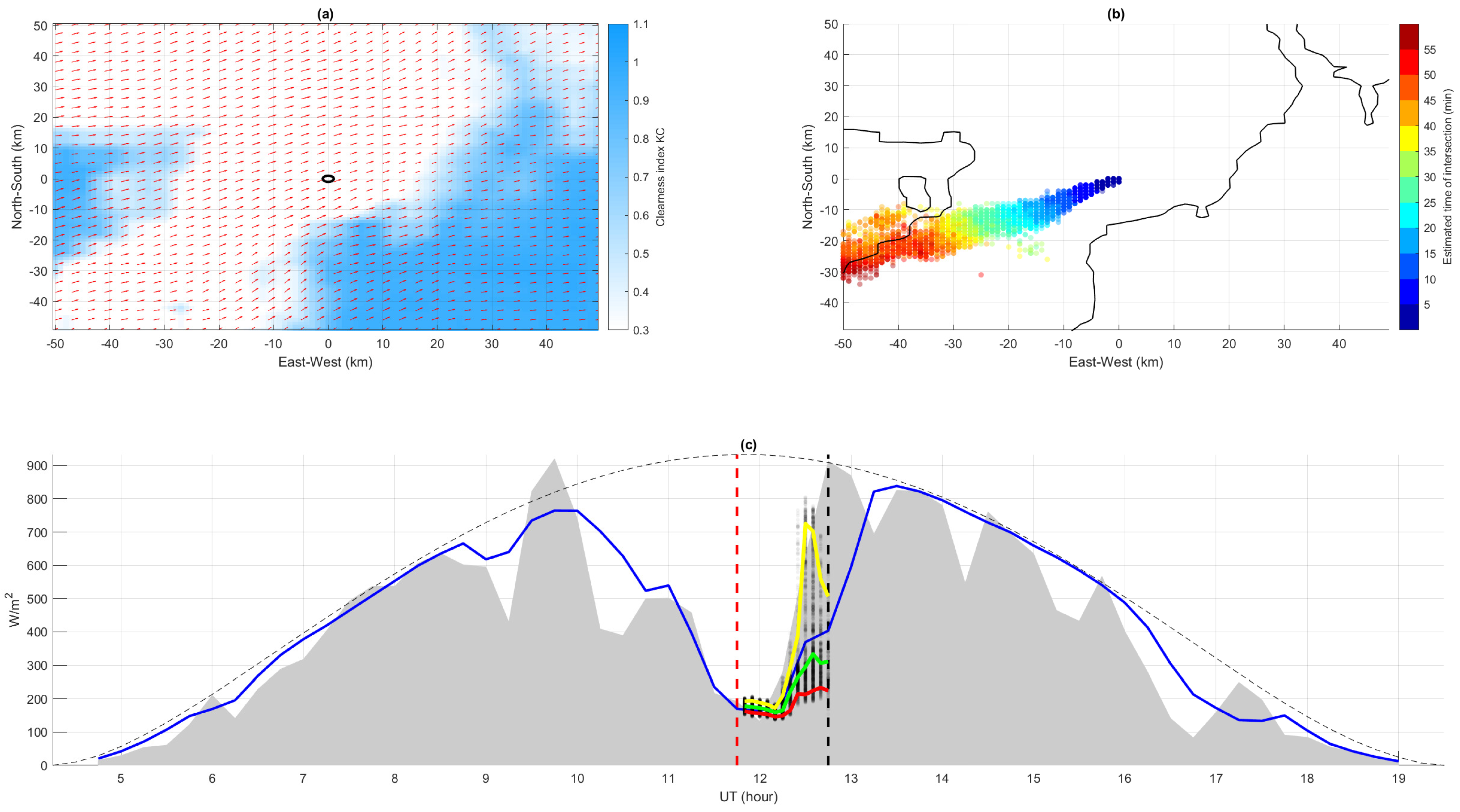
In this section, we present the method we developed to obtain probabilistic forecasts of Global Horizontal Irradiance (GHI) at a given location. This method consists of four steps:

• calculation of the clear-sky index $k_c$ for each pixel of a given satellite sub-image, centered at the location of interest with a radius of typically 50 km to 100 km; n this paper, a radius of roughly 50 km is used;
• estimation of the Cloud Motion Vectors (CMV) using an approach of Optical Flow (OF);
• identification of the pixels that are likely to advect to the location of interest for different time horizons (named hereinafter upcoming or converging $k_c$ pixels or values); and
• building of the Probability Distribution Function (PDF) of the upcoming $k_c$ based on the candidate pixels.

2.1. Calculation of the Clear-Sky Index $k_c$

The first step is to estimate the clear-sky index $k_c$ from images of upwelling radiance acquired every 15 min by the sensor SEVIRI on the geostationary satellite Meteosat Second Generation at longitude $0^{\circ }$. The clear-sky index is defined as:

$$k_c=\frac{GHI}{GH{I}_{cls}},$$

(1)

where $GH{I}_{cls}$ is the GHI under clear-sky conditions. Thus, the $k_c$ varies between 1 when the sky is perfectly clear to values close to 0 in overcast conditions. To assess this clear-sky index from the satellite images, we use the Heliosat-2 method [40].

2.2. Identification of the Cloud Motion Vectors

To obtain the motion vectors of the pixels of the transformed satellite images, we used an OF technique. This technique refers to the apparent motion of patterns in a sequence of images that results from the individual motions moving objects in the observed scene. This means that 3D movements are summarized to 2D flows that can be evaluated using image processing techniques. OF methods use two consecutive images to derive the motion vectors, and have been in use for a long time, with a wealth of related publications [41].

The basic assumption of the OF method is the brightness constancy assumption. Assuming that the picture is a field of intensity values for each pixel located with coordinates $(x,y)$ at a time t, i.e., $I(x,y,t)$, the brightness constancy states that:

$$I(x+dx,y+dy,t+dt)=I(x,y,t).$$

(2)

This assumption means that the intensity structures will remain the same between two consecutive images, which can be decomposed in two points: (i) that there is no change in lighting between two images (thus, $k_c$ is used instead of GHI, which can also be derived from the Heliosat-2 method but is more sensitive to the Sun relative position); and (ii) that no clouds are supposed to appear, disappear or transform between two consecutive images. Using a first-order Taylor expansion, this assumption writes:

$$\frac{\partial I}{\partial x}dx+\frac{\partial I}{\partial y}dy+\frac{\partial I}{\partial t}dt=0.$$

(3)

The elements that we want to identify are the pixel velocities $v_x=\frac{dx}{dt}$ and $v_y=\frac{dy}{dt}$. Rewriting the brightness constancy assumption gives:

$$\frac{\partial I}{\partial x}{v}_x+\frac{\partial I}{\partial y}{v}_y+\frac{\partial I}{\partial t}=0.$$

(4)

The x- and y-derivatives $\frac{\partial I}{\partial x}$ and $\frac{\partial I}{\partial y}$ can be estimated from the current picture, and the temporal derivative $\frac{\partial I}{\partial t}$ can be estimated from two consecutive pictures. There are then two unknowns, $v_x$ and $v_y$, and one equation, so that one additional constraint is required to derive the motion vectors (ill-posed problem).

There are various methods used to obtain a well-designed system to eventually derive the motion vectors, notably the use of a regularization term [41]. In this paper, we pursued the work of Reference [42] and used an efficient method from Reference [43] which combines a Gaussian-pyramid-based coarse-to-fine approach with Iteratively Reweighted Least Squares (IRLS).

In addition, many works showed that smoothing is beneficial to CMV approaches using OF, as it reduces spatial uncertainty [44]. In the typical spatial smoothing, all pixels in the neighborhood are typically used to smooth a forecast field. It results in a very smooth forecast that will minimize the risk of high error values. However, in our approach, we do not consider all pixels in the neighborhood but, rather, selected pixels based on the characteristics of the optical flow. A second difference is that, while the smoothing approach takes the average values, our algorithm provides the probability distribution of the forecast value, which contains more information. If we take the ensemble mean, our approach would be very close to the well-known smoothing approach. From this perspective, our approach can be thought of as a generalization of the smoothing approach, which contains more information, so we did not used standard spatial smoothing.

2.3. Identification of the Candidate Pixels

Once we derived the clear-sky index $k_c$ for each pixel, along with the motion vectors $v_x$ and $v_y$, the next step is to identify the pixels that can potentially have an impact on the location of interest. To do so, we define a monitored perimeter around this location of interest. Then, we compute for each pixel if the motion indicates that it will enter this perimeter, and at what time. It is important to note that to perform this computation, we use an Eulerian approach where each pixel is assumed to have a constant motion vector and to move in a straight line. Many works using CMV approaches consider, rather, a Lagrangian approach, where each pixel moves in the motion field and, thus, follows a trajectory that can be different from a straight line. However, Eulerian approach is simpler and more efficient to compute; since we are working on forecast horizons shorter than 1 h, no significant difference is to be expected between the two approaches.

For each forecast horizon, we can determine the pixels that can potentially have an impact for that forecast horizon, and we consider that the $k_c$ values identified for these pixels are plausible values for the upcoming $k_c$ values at the location of interest.

Standard CMV-based forecasting approaches generally proceeds in a different way. Indeed, as described by the recent paper from Reference [38], a standard CMV-based forecasting approach uses CMV to “extrapolate the cloud index map” from the time when the forecast is initiated to the leading time. This extrapolation is performed with a simple 2D resampling, generally followed by the application of a smoothing kernel.

This “forward” extrapolation approach presents the advantage of providing forecasted cloud-index maps for each pixel at the same time. However, this approach does not handle CMV situations when different locations appears to “converge” for the same time of horizon to the monitored perimeter. Depending on the implementation of the resampling, this procedure will, at best, do an average on the converging $k_c$ values and more plausible a “random choice” of the $k_c$ value eventually selected.

The proposed approach is a “backward” one, i.e., on the contrary, centered to a given monitored perimeter of interest and is enabled to handle explicitly situations of convergence from different locations as superposition of possible states as an ensemble of plausible clear-sky indexes, from which will be derived empirical Cumulative Distribution Function (CDF).

Considering a cloud on a pixel with coordinates $(x,y)$ and motion components $v_x$ and $v_y$, we can estimate the distance at time t between the cloud and the location of interest at coordinates $(0,0)$ with:

$$d\left(t\right)=\sqrt{{(x+t{v}_x)}^2+{(y+t{v}_y)}^2}.$$

(5)

By equating the derivative of this distance with respect to time to 0, we can find the time for which this distance is the smallest with:

$$t_{closest}=-\frac{x{v}_x+y{v}_y}{v_x^2+v_y^2}.$$

(6)

Then, the distance between the cloud and the sensor at that time is:

$$\begin{array}{cc}\hfill d_{closest}& =d\left(t_{closest}\right)=\hfill \end{array}$$

(7)

$$\begin{array}{cc}\hfill & \sqrt{{(x+v_x{t}_{closest})}^2+{(y+v_y{t}_{closest})}^2}.\hfill \end{array}$$

(8)

So, the candidate pixels that can potentially impact at the location of interest between future times $t_1$ and $t_2$ are identified with the condition:

$$t_1\le t_{closest}\le t_2 \mathrm{and} d_{closest}\le R_m,$$

(9)

where $R_m$ is the radius of the monitoring perimeter.

To improve the calibration properties of the probabilistic forecasts, we followed a Monte-Carlo procedure by adding a centered Gaussian noise to the norm and direction of the motion vectors. We consider that the noise realization is the same over each image. For a given image, an error on the motion vector direction and norm $d\theta$ and $dr$ are drawn from a centered Gaussian distribution. Then, the new motion vectors can be estimated as:

$$\begin{array}{c}\hfill v_x^{{}^{\prime }}=\sqrt{v_x^2+v_y^2+dr}\ast cos\left(ta{n}^{-1}\left(\frac{v_y}{v_x}\right)+d\theta \right),\end{array}$$

(10)

$$\begin{array}{c}\hfill v_y^{{}^{\prime }}=\sqrt{v_x^2+v_y^2+dr}\ast sin\left(ta{n}^{-1}\left(\frac{v_y}{v_x}\right)+d\theta \right).\end{array}$$

(11)

Thus, to obtain the candidate pixels, we identify the pixels that satisfy the conditions from Equation (9) not only for the motion vector map calculated with the OF method but also for an arbitrary number of maps $N_{mc}$ obtained by drawing the noise of the motion vectors $N_{mc}$ times.

This Monte-Carlo procedure improves the calibration properties of the model. Since we draw the error components from centered Gaussian distribution i.e., $dr\sim \mathcal{N}(0,{\sigma }_r),d\theta \sim \mathcal{N}(0,{\sigma }_{\theta })$, the application of the Monte-Carlo procedure requires the estimation of two additional parameters, ${\sigma }_r$ and ${\sigma }_{\theta }$.

We found that standard quadratic error measures, such as the Continuous Ranked Probability Score (CRPS; see definition in Section 3) tend to favor smooth forecasts that avoid large errors. Using an optimization loop with such criteria to obtain optimized parameters would then result in very large parameters, so the noise added would be very important. In the end, forecasts would simply be the average of the satellite pictures, and all information about the cloud motions would be lost. A similar trade-off has been reported for deterministic settings when performance assessment relies in quadratic error measures (such as CRPS) [45]. Such metrics tend to favor smooth forecasts as to avoid large errors. Devising an adequate error measure is a research task on its own, and it is out of the scope of this work.

Thus, we adopted a trial-and-error approach to estimate the parameters, while having the physical mechanisms at play in consideration:

• a standard deviation of 2 km/h for the Gaussian noise added to the cloud speed (${\sigma }_r$), which is roughly one order of magnitude lower than the typical wind speed in the lower atmosphere (a few dozen km/h);
• a standard deviation of $\pi /12$ radians for the Gaussian noise added to the cloud direction (${\sigma }_{theta}$); significantly higher values were considered, as to represent the difficulty in accurately estimating a CMV and the fact that it varies over time (which the Eulerian approach here used disregards), but larger values resulted in the loss of all information regarding trajectories (i.e., considerably worse sharpness values); and
• a monitoring radius of 1 km, intentionally lower than the 3 km satellite resolution; larger values increase the number of selected candidates (with the new ones being farther from the sensor location), which would then describe a variability that is less similar to that of a point sensor.

Regarding the monitoring perimeter, it is important to emphasize that these parameters consider not the original position of a given neighboring pixel but, instead, where it would be after considering a given CMV and time interval. Thus, it should be seen as giving some flexibility to the candidate selection process, as it is very unlikely that any advected pixel overlaps perfectly with the sensor. At the same time, it accounts for CMV uncertainty as a perimeter deems a range of vectors as suitable candidates (i.e., compliant with this selection criterion).

Additionally, we chose a single set of parameters which lead to good performance and reliability for the two test locations as to avoid overfitting and further validate the model (and its parameter choice). Although extremely high or low values result in bad quality forecasts, we found that, once reasonable values were found, the resulting forecasts were not much sensitive to these parameters. This explains why the same parameters could be used for two different locations with similar forecasting performance.

2.4. Building of the Empirical Distribution of the Clear-Sky Index $k_c$

Once we obtained a set of candidate pixels, we consider that the corresponding $k_c$ values are plausible for the location of interest at a given horizon. However, to improve the calibration of the forecasting system, we add a Heliosat-2 $k_c$ estimation error component. To do so, estimation errors are collected at the location of interest based on the GHI measurements and the corresponding Heliosat-2 $k_c$ estimations on a training set. The CDF of these errors is then estimated conditionally to the Sun’s elevation and the level of $k_c$. To do so, both the Sun’s elevation and the $k_c$ level were binned into 5 intervals of equal population (i.e., intervals defined by the 20th, 40th, 60th, 80th, and 100th quantiles). This results in 25 possible CDFs. When an additional noise is drawn for the $k_c$ at a given pixel, it is drawn from the appropriate CDF, depending on the $k_c$ level of that pixel and the Sun’s elevation at the time when the image was acquired. This constitutes a second loop of Monte-Carlo drawings.

The $k_c$ values of the candidate pixels calibrated with an estimation error component define a set of candidate clear-sky indexes $k_{c_{candidates}}$. We consider that the closest the cloud passes from the location of interest, the more plausible its $k_c$ value is. Thus, we construct the CDF as the empirical CDF of the set $k_{c_{candidates}}$, each $k_c$ being weighted by the inverse of $d_{candidates}$, the minimal distance at which the cloud passes, computed by Equation (7).

In other words, the CDF is computed as:

$$\begin{array}{cc}\hfill w_i& =\frac{1}{d_{candidates,i}},\hfill \end{array}$$

(12)

$$\begin{array}{cc}\hfill CDF\left(x\right)& =\frac{{\sum }_i{w}_{i|k_{c_{candidates,i}}\le x}}{{\sum }_i{w}_i}.\hfill \end{array}$$

(13)

This is the same as modeling the PDF as a sum of Dirac distributions with weights $w_i$:

$$PDF\left(x\right)=\sum _i{w}_i\delta \left(x-k_{c_{candidates,i}}\right).$$

(14)

Finally, we can obtain the CDF of the irradiance by multiplying the clear-sky index of the CDF by the clear-sky GHI which was estimated using the McClear model, notably accounting for water vapor and aerosol effects as forcasted by Copernicus Atmospheric Monitoring Services (CAMS) [46].

For illustration purposes, Figure 1 presents a “snapshot” of the CMV-based probabilistic forecasting for one of the considered test locations, described in more detail in a later section, for an arbitrary date (11 July 2016). at 12:00 UT and 1-h ahead horizon. An overall flowchart summarizing all the components of the method is proposed in Figure 2.

3. Performance Assessment

The proposed probabilistic forecasting approach is evaluated in both a deterministic and a probabilistic setting. We used the following acronyms in the evaluation section:

• The proposed probabilistic CMV approach is noted Pr-CMV.
• We can also provide deterministic forecasts using the Pr-CMV, by taking the median of the forecast distribution as the deterministic forecast. This method of obtaining deterministic forecasts is noted Pr-CMV-Det.

We also used several baseline models to compare with our approach. These are:

• A standard CMV approach with no Monte-Carlo procedure noted St-CMV. With this method, the motion vectors are propagated assuming an Eulerian approach to estimate the upcoming GHI map for the next time step.
• Two baseline models that make no use of satellite information: the Smart Persistence model noted persistence, for deterministic evaluation, and the Complete-History Persistence Ensemble noted CH-PeEn, for probabilistic evaluation. These models are defined in Section 3.2.

The deterministic evaluation is essentially performed as a preliminary validation step. As the median motion vectors of the probabilistic approach are identical to a traditional CMV, using the Pr-CMV-Det approach is expected to perform similarly to the deterministic St-CMV.

3.1. Metrics

Three classical normalized indicators of performance for the deterministic evaluation were considered: the normalized bias ($nBIAS$); the normalized mean absolute error ($nMAE$); and the normalized root mean squared error ($nRMSE$). These are notably defined in Reference [47], and, in this paper, the normalization is performed relative to the mean value of the observations of daylight period (i.e., when the sun elevation is larger than ${10}^{\circ }$.

Evaluating the performance of probabilistic forecasts is considerably more complex than deterministic forecasts as there are numerous desirable properties which can be contradictory to each other. In this paper, we follow the evaluation paradigm presented in Reference [48], focusing on the reliability and sharpness of a forecasting model.

Reliability is defined as the consistency between the forecast probability of a given event and its observed frequency. This is assessed using reliability diagrams, where the empirical frequency of the quantiles obtained on the testing set are plotted against their nominal quantile levels. For example, for the quantile of level $25\%$, we quantify the frequency at which the ground measurement fall below the $25\%$ level quantile and plot it against the value $0.25$. For a perfectly reliable forecast, the measurement should fall below the forecast quantile of level $\alpha$ exactly $\alpha \%$ of the time. Visually, the diagram of a perfectly reliable system corresponds to an identity line, whereas large deviations from this indicate a lack of calibration. Deviations from the diagonal line can also occur because of the finite size of the testing set. To address this, we use Reference [49] to draw intervals that show the range in which a perfectly calibrated system could be located due to the finite size of the evaluation set with a $\alpha =5\%$ confidence level. This means that any deviations outside the interval allow us to reject the null hypothesis that the probabilistic CMV is perfectly calibrated, with a $5\%$ significance level.

To numerically quantify the reliability property, we use the Mean Reliability Deviation (MRD), which is the mean of the absolute deviations between the diagonal line and the actual reliability diagram. For a set of N quantile $q_{\alpha }$ of levels $\alpha$ and their actual frequencies $\widehat{\alpha }$, the MRD is defined as:

$$MRD=\frac{1}{N}\sum |\alpha -\widehat{\alpha }|.$$

(15)

While the reliability property is highly desirable, it does not guarantee a model is of practical use. For example, a climatological model that forecasts each quantile of the upcoming distribution as the empirical quantile observed on a given training set is perfectly reliable, although it contains no predictive information besides the averages of the training set. Thus, it is important to assess a model’s sharpness, as it quantifies the typical width of the forecast distribution. While a climatological system has a perfect reliability, it has a very low sharpness since it considers all observations from the training set equally, so that the forecast interval is large. On the other hand, a model that has forecasts conditional to some predictive exogenous inputs is generally sharper.

Sharpness is quantified using the Prediction Interval Normalized Average Width (PINAW), which is the average width of the interquantile for a given level of confidence. For a confidence level $\beta$, and a number $N_f$ of quantile forecasts $\widehat{q}$, along with the GHI measurements $y_i$, the PINAW is defined as:

$$PINA{W}_{\beta }=\frac{1}{N_f}\sum _{i=1}^{N_f}\frac{{\widehat{q_i}}_{1-\beta /2}-{\widehat{q_i}}_{\beta /2}}{y_i}.$$

(16)

In our evaluation, we will also use the Mean Prediction Interval Normalized Average Width ($MPINAW$), which is the average $PINAW$ over all possible $\beta$ values, given the available forecast quantiles:

$$MPINAW=\overline{PINA{W}_{\beta }}.$$

(17)

Both concepts are often contradictory: improving the reliability of a model can worsen its sharpness and vice-versa. However, forecasts can always be re-calibrated to have a good reliability, while sharpness is usually an inherent property of the forecasting model that can not be modified. Thus, in Reference [48], it is stated that reliability should be a requisite for a model, while sharpness should be quantified after verifying that the model is reliable. Thus, we will first evaluate the reliability of the probabilistic CMV, and then we assess its sharpness.

Finally, the Continuous Rank Probabilistic Score (CRPS), a composite metric which considers both reliability and sharpness, is calculated. For a forecast CDF F and a verification value y, the CDF is defined as:

$$CRPS={\int }_{-\infty }^{\infty }{\left(F\left(x\right)-1_{\{y\le x\}}\right)}^{2}dx.$$

(18)

The CRPS is then derived for each individual forecast, and the average value is considered. In this work, the CRPS is presented in %, with respect to the mean value of GHI during the daylight periods, over the whole dataset of reference.

3.2. Baseline Models

As a deterministic baseline, the smart persistence (Persistence) model was considered, which can be defined as follows:

$$GH{I}_{Pers}(t+h)=k_c\left(t\right)GH{I}_{cls}(t+h),\forall h.$$

(19)

For probabilistic forecasting, the Complete-History Persistence Ensemble (CH-PeEn) [50] was considered. The CH-PeEn consists of building an ensemble of $k_c$ values by taking all the $k_c$ in the history that have the same forecast time, independently of the lead time (i.e., no dependency with respect the time horizon). For example, to perform a forecast for a given day at 09:00 a.m., all the available $k_c$ values measured at the same time of day are used to build the ensemble. The quantiles of the distribution are then computed as the empirical quantiles of the ensemble. Thus, the forecast distribution depends only on the time of the day.

3.3. Data

To perform our probabilistic forecasts, we used data from two sites located in France. For each case, we have ground-based GHI measurements from pyranometers, as well as satellite-derived GHI maps on radius larger than 50 km around the locations of the sensors. The characteristics of both sites and the period for which data is available are summarized in

Table 1. Summary of the sites location and description of the yearly dataset of measured 15-min GHI used for training and for evaluation.

Location	Latitude (°)	Longitude (°)	Elevation (m)	Training Period	Evaluation Period
Carpentras	44.0830	5.0590	100	2015: 14,573 data	2016: 13,995 data
Signes	43.25551	5.8	441	2015: 14,686 data	2016: 13,693 data

.

The satellite-derived data used are time-series of GHI maps with a native time step of 15 min and a spatial resolution of approximately 3 × 4.5 km. This satellite dataset has been extracted from the database HelioClim-3 version 5, based on the Heliosat-2 method applied on images from the sensor SEVIRI of Meteosat Second Generation ($0^{\circ }$ Service). This database available online at http://www.soda-pro.com (last access: 23 June 2021) and is used both for research and industrial developments. It can be used for historical analysis, starting at February 2014 up to the current day, and is also available at near real-time with a time lag of less than few minutes. Numerous validation and performance analyses of HelioClim-3 for different regions and climates have been performed [51,52,53,54] and demonstrate the good reliability of this database to capture the spatial and temporal variability of the surface solar irradiance.

The ground-based measurements of GHI used as reference are first quality-checked at their native time resolution: 1-min and 5-min time steps, respectively, for Carpentras and Signes. This quality check first uses an automatic procedure based on upper and lower limits for extremely rare intervals, as described by Reference [55], and then on a visual inspection. These time-series of GHI are then averaged to 15-min to be consistent with the satellite data acquired every 15-min. Only data corresponding to a sun elevation angle larger than ${10}^{\circ }$ is considered both for ground measurements and satellite estimations.

Due to the native time resolution of the considered data, forecasts were completed for 15-min intervals, up to a 1-h horizon. However, it is important to note that, just as in the deterministic CMV-based models, the Pr-CMV is very flexible: without being constrained by the resolution of the data, it can be adapted to any choice of time horizons.

The CDF of the Heliosat-2 estimation errors are obtained based on a whole year used for the training period (2015), different for the whole year 2016 used for the performance analyses, in order to have a dataset representative for the four seasons. The values of the different parameters required in the simulation are reported in

Table 2. Parameters used in the simulations.

${\mathit{\sigma }}_{\mathit{r}}$ (km/h)	${\mathit{\sigma }}_{\mathit{\theta }}$ (radians)	${\mathit{R}}_{\mathit{m}}$ (km)	${\mathit{N}}_{\mathit{mc}}$
2	$\pi$/12	1	5000

.

3.4. Deterministic Performance

As discussed in Section 3, a preliminary validation of the proposed approach is performed by comparing its deterministic performance to the St-CMV model. All the indicators are computed and then reported in

Table 3. Evaluation results.

Deterministic Evaluation (Carpentras)
Category (reference value)	Low variability days 217 days (540.3 W/m${}^2$)					High variability days 148 days (441.3 W/m${}^2$)					All days 365 days (500.2 W/m${}^2$)
Horizon (minutes)	15	30	45	60	All	15	30	45	60	All	15	30	45	60	All
nBIAS - Persistence (%)	0	−0.1	−0.2	−0.4	−0.2	0.1	0.1	−0.1	−0.3	0	0	0	−0.2	−0.4	−0.1
nBIAS - St-CMV (%)	0.2	0	−0.3	−0.8	−0.2	0	−0.2	−0.4	-1	−0.4	0.1	−0.1	−0.4	−0.9	−0.3
nBIAS - Det-Pr-CMV (%)	0.3	0	−0.4	−0.9	−0.2	0.9	0.2	−0.6	−1.7	−0.3	0.5	0.1	−0.5	−1.2	−0.3
nMAE - Persistence (%)	2.6	3.5	4.2	4.9	3.8	16.1	21.7	25	27.2	22.6	7.4	10.1	11.7	12.9	10.5
nMAE - St-CMV (%)	4	4.4	4.9	5.6	4.7	17.2	19.5	22.2	24.7	20.9	8.7	9.8	11.1	12.5	10.5
nMAE - Det-Pr-CMV (%)	4	4.3	4.9	5.6	4.7	17	18.3	19.9	21.9	19.3	8.6	9.3	10.3	11.4	9.9
nRMSE - Persistence (%)	6.2	8	9.3	10.5	8.6	24.8	32.1	36.2	38.9	33.5	14.9	19.2	21.8	23.6	20.1
nRMSE - St-CMV (%)	7.2	8.2	9.2	10.4	8.8	24.5	27.6	31.2	34.3	29.7	15	16.9	19.1	21.2	18.2
nRMSE - Det-Pr-CMV (%)	7.1	7.7	8.8	9.9	8.4	24.3	25.7	27.7	30.2	27.1	14.9	15.8	17.2	18.8	16.7
Probabilistic Evaluation (Carpentras)
Category (reference value)	Low variability days 217 days (540.3 W/m${}^2$)					High variability days 148 days (441.3 W/m${}^2$)					All days 365 days (500.2 W/m${}^2$)
Horizon (minutes)	15	30	45	60	All	15	30	45	60	All	15	30	45	60	All
MRD - CH-PeEn (%)	8.4	8.4	8.4	8.4	8.4	12.2	12.2	12.2	12.2	12.2	0.1	0.1	0.1	0.1	0.1
MRD - Pr-CMV (%)	5.2	4.8	5.2	6.5	4.7	5.3	5.9	6.5	7.3	6.3	2.2	3.5	4.8	6	4.1
MPINAW - CH-PeEn (%)	46.1	46.1	46.1	46.1	46.1	57.1	57.1	57.1	57.1	57.1	50.2	50.2	50.2	50.2	50.2
MPINAW - Pr-CMV (%)	11.3	11.7	12.0	12.6	11.8	22.9	25.0	27.4	29.1	26.1	15.4	16.4	17.6	18.6	17.0
CRPS - CH-PeEn (%)	13.8	13.8	13.8	13.8	13.8	25.2	25.2	25.2	25.2	25.2	17.8	17.8	17.8	17.8	17.8
CRPS - Pr-CMV (%)	3.2	3.5	3.9	4.4	3.7	12.8	13.6	14.8	16.2	14.3	6.6	7.1	7.8	8.6	7.5
Deterministic Evaluation (Signes)
Category (reference value)	Low variability days 178 days (599.2 W/m${}^2$)					High variability days 187 days (452.1 W/m${}^2$)					All days (530.7 W/m${}^2$)
Horizon (minutes)	15	30	45	60	All	15	30	45	60	All	15	30	45	60	All
nBIAS - Persistence (%)	0.5	0.8	1	0.9	0.8	0.4	0.7	0.9	0.8	0.7	0.5	0.8	0.9	0.8	0.7
nBIAS - St-CMV (%)	0.7	0.5	0.2	−0.4	0.3	1.7	1.6	1.3	0.6	1.3	1.1	0.9	0.6	0	0.7
nBIAS - Det-Pr-CMV (%)	0.7	0.5	0	−0.8	0.1	1.4	1.4	0.7	−0.1	0.8	0.9	0.9	0.3	−0.5	0.4
nMAE - Persistence (%)	2.6	3.8	4.8	5.8	4.2	17.8	23.5	26.3	28.6	24.1	8.6	11.6	13.3	14.8	12.1
nMAE - St-CMV (%)	6.5	6.8	7.3	8.3	7.2	19.9	22.6	24.9	27	23.6	11.8	13.1	14.3	15.5	13.7
nMAE - Det-Pr-CMV (%)	6.5	6.9	7.5	8.2	7.3	19.6	21.7	23.2	25.1	22.4	11.7	12.8	13.7	14.9	13.3
nRMSE - Persistence (%)	5.7	7.6	8.9	10	8.2	27.2	34.7	38	40.5	35.4	16.5	21.1	23.2	24.9	21.7
nRMSE - St-CMV (%)	8.9	9.5	10.2	11.3	10	28	31.6	34.8	37.4	33.1	17.8	20	21.9	23.6	21
nRMSE - Det-Pr-CMV (%)	8.8	9.5	10.3	11.6	10.1	27.4	30.2	32.4	34.7	31.3	17.5	19.2	20.6	22.3	20
Probabilistic Evaluation (Signes)
Category (reference value)	Low variability days 178 days (599.2 W/m${}^2$)					High variability days 187 days (452.1 W/m${}^2$)					All days (530.7 W/m${}^2$)
Horizon (minutes)	15	30	45	60	All	15	30	45	60	All	15	30	45	60	All
MRD - CH-PeEn (%)	10	10	10	10	10	11	11	11	11	11	0.2	0.2	0.2	0.2	0.2
MRD - Pr-CMV (%)	2	1.5	2.1	3	2.1	432	4.7	4.7	5.1	4.6	1.3	1.7	2	2.8	1.8
MPINAW - CH-PeEn (%)	45.6	45.6	45.6	45.6	45.6	58.0	58.0	58.0	58.0	58.0	50.5	50.5	50.5	50.5	50.5
MPINAW - Pr-CMV (%)	16.3	16.7	17.0	17.5	16.9	28.0	29.9	32.2	33.9	31.0	20.9	21.9	23.1	24.0	22.5
CRPS - CH-PeEn (%)	12.8	12.8	12.8	12.8	12.8	25.0	25.0	25.0	25.0	25.0	17.6	17.6	17.6	17.6	17.6
CRPS - Pr-CMV (%)	4.9	5.2	5.6	6.2	5.5	14.4	15.7	17.0	18.4	16.4	8.6	9.4	10.1	11.0	9.8

. They are reported depending on forecast horizon and class of day variability.

This classification is based on a simple threshold for the mean of absolute $k_c$ variations over a given day. To estimate the threshold, we realized a scatter plot of the mean $k_c$ variation against the irradiation level. We found a threshold of 0.075, which we believe to separate well the days when persistence is most efficient (either very cloudy or sunny days, i.e., low or high mean daily $k_c$), from the more variable days. Thus, low variability days were considered those with a mean $k_c$ variation below 0.075.

The results over all forecast horizons are summarized in Table 3. On average, persistence-based forecasts perform better for low variability days and for horizons shorter than 30 min, while the CMV-based forecasts perform better for high variability days and horizons longer than 30 min. This is in accordance with literature results that recommend the use of in-situ measurements for better forecast performance in the very short term, as well as satellite imagery for larger horizon ranges.

All the proposed models have very good calibration properties with low nBIAS values. However, the persistence model seems to have the best calibration properties, with a nBIAS always lower than 1%, while it can go up to 2% for the CMV-based forecasts. There is also a trend that the persistence generally performs better in terms of nMAE, while the CMV has a lower spread and performs better in terms of RMSE.

Finally, the Pr-CMV-Det behaves as expected: the difference between the two satellite-based approaches is minimal, so there is no drawback to using the Pr-CMV in a deterministic setting, as the performance is very similar to a standard one.

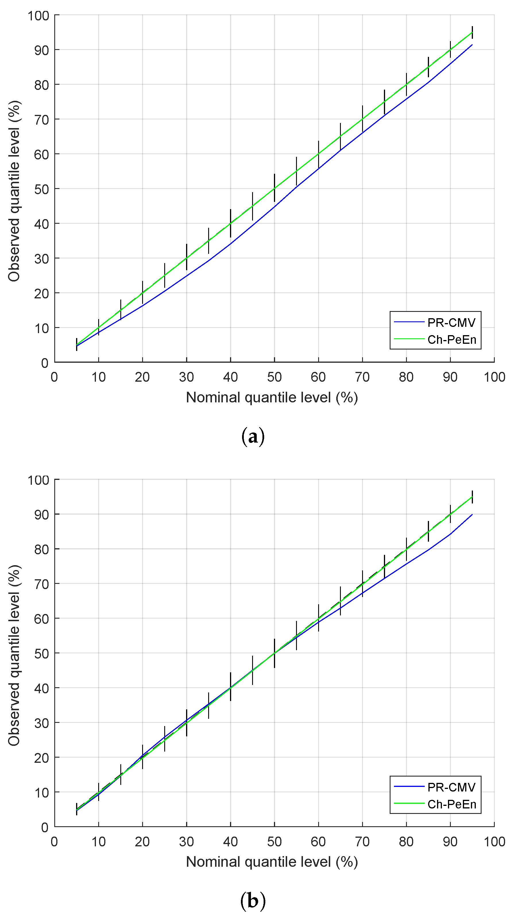
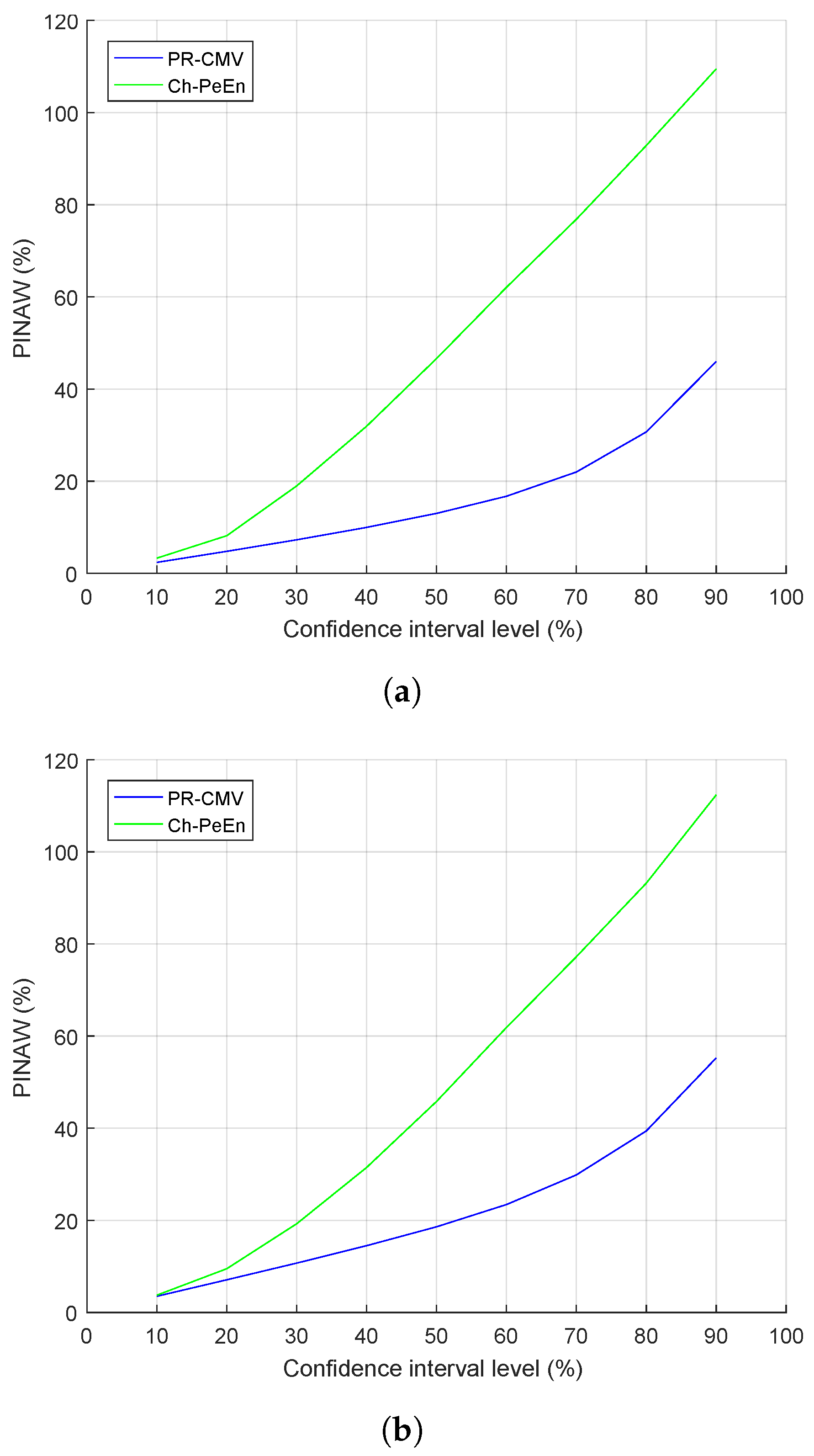
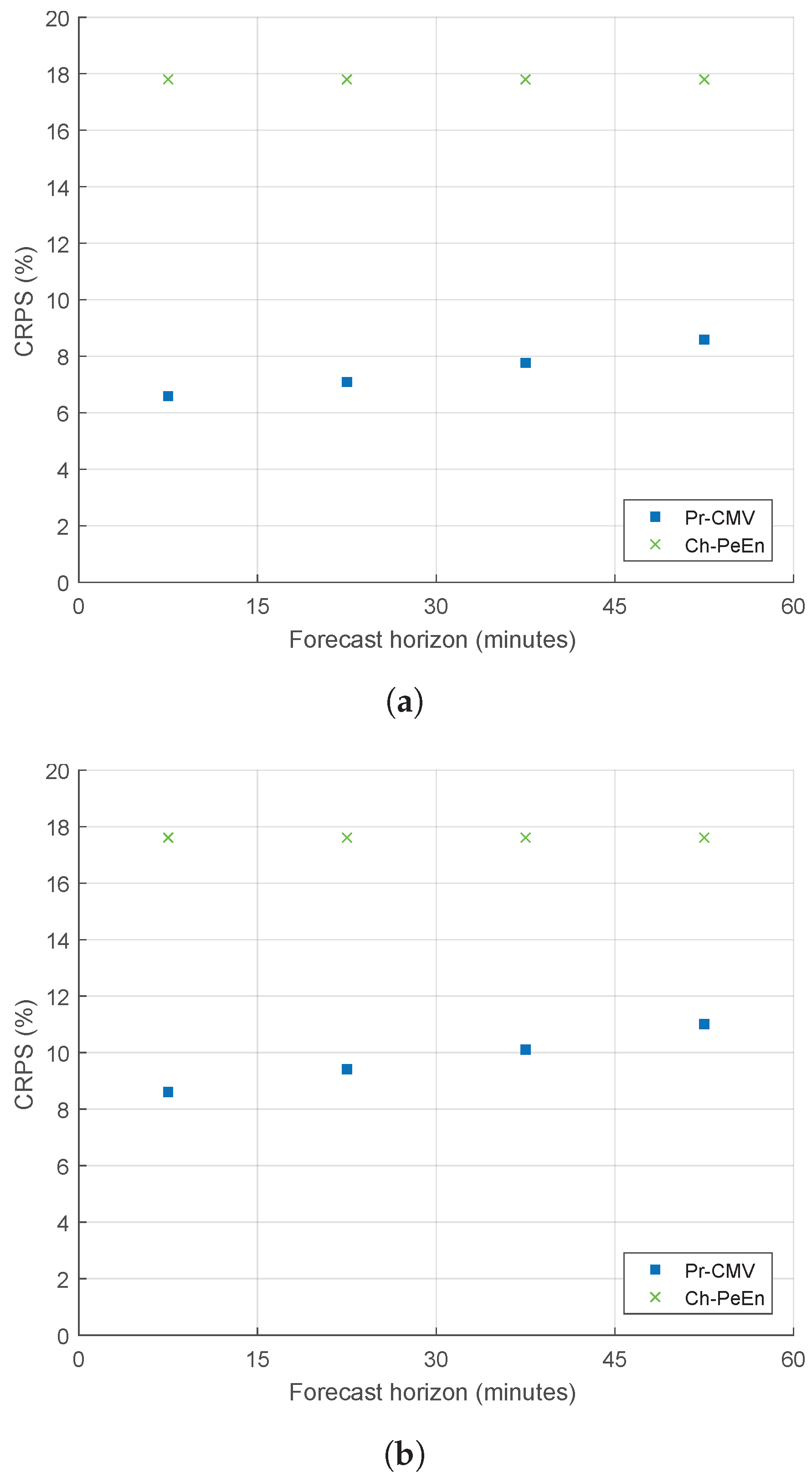
3.5. Probabilistic Performance

We derived the reliability diagrams, the PINAW, and the CRPS of the Pr-CMV and CH-PeEn models. The results are presented in Table 3, and reliability, sharpness, and CRPS, with the two latter being presented by time horizon every 15 min up to 1 h, for the two sites, which are presented, respectively, by Figure 3, Figure 4 and Figure 5.

Results show that the calibration of the CH-PeEn is better, on average, with very low MRD values. However, when comparing the models depending on the day variability, the reliability of the CH-PeEn decreases, while the reliability of the Pr-CMV remains similar. In any case, both models show sufficient reliability properties, with deviations from the diagonal line lower than 10%, in the worst case.

Plotting the reliability diagrams reveals further that, for Carpentras, there is a global tendency of underestimating the forecasts. For the Signes power plant, the lower-level quantiles of the CDF are slightly overestimated, while the higher-level quantiles are underestimated. This results in a forecast distribution that is globally too narrow. These issues could be corrected with a fine tuning of the parameters ${\sigma }_r$, ${\sigma }_{\theta }$, and $R_m$.

On the other hand, the forecasts from the Pr-CMV are much sharper than the CH-PeEn, which seems natural as the CH-PeEn uses all the history for computing the forecasts independently on the state of the atmosphere, which results in very wide forecast intervals, as for a climatological forecast. However, an increase in sharpness is not necessarily an improvement, as it can be obtained at the cost of decreasing the reliability. By computing the CRPS, we can assess if the forecast from the Pr-CMV is closer to the true distribution than the CH-PeEn. The CRPS values are indeed lower for the Pr-CMV for any time horizon and any class of days than the CH-PeEn, which ultimately proves that the cloud motion modeling step that we added in the Pr-CMV method effectively has an added value compared to a naive method, such as the CH-PeEn.

4. Conclusions

This paper addresses the difficulty in estimating the uncertainty in the upcoming irradiance for forecast horizons shorter than one hour. In this horizon range, forecasts are typically obtained by using in-situ measurements, which contain few predictive information on the future state of the atmosphere. This ultimately results in forecast intervals that are too narrow and do not accurately represent the upcoming uncertainty.

Several approaches use satellite information to incorporate knowledge of the future state of the atmosphere, thanks to its spatial and temporal perspectives. However, they provide deterministic forecasts, while most decision-making problems in the energy sector require estimation of the uncertainty.

In this paper, we propose a probabilistic forecast model that uses satellite information and generates probabilistic forecasts. We showed that this model performs well compared to standard CMV approaches in a deterministic setting. Besides, it has good probabilistic properties, so the uncertainty information it provides can be reliably used in a decision-making problem. The paper does not intend to propose a definitive method but, rather, aims at opening a new way of using CMV for short-term probabilistic forecasting using satellite as a source of real-time observation.

References

1. Wu, J.; Botterud, A.; Mills, A.; Zhou, Z.; Hodge, B.M.; Heaney, M. Integrating solar PV (photovoltaics) in utility system operations: Analytical framework and Arizona case study. Energy 2015, 85, 1–9. [Google Scholar] [CrossRef] [Green Version]
2. Notton, G.; Nivet, M.L.; Voyant, C.; Paoli, C.; Darras, C.; Motte, F.; Fouilloy, A. Intermittent and stochastic character of renewable energy sources: Consequences, cost of intermittence and benefit of forecasting. Renew. Sustain. Energy Rev. 2018, 87, 96–105. [Google Scholar] [CrossRef]
3. Litjens, G.; Worrell, E.; van Sark, W. Assessment of forecasting methods on performance of photovoltaic-battery systems. Appl. Energy 2018, 221, 358–373. [Google Scholar] [CrossRef]
4. Masa-Bote, D.; Castillo-Cagigal, M.; Matallanas, E.; Caamaño-Martín, E.; Gutiérrez, A.; Monasterio-Huelín, F.; Jiménez-Leube, J. Improving photovoltaics grid integration through short time forecasting and self-consumption. Appl. Energy 2014, 125, 103–113. [Google Scholar] [CrossRef] [Green Version]
5. Antonanzas, J.; Pozo-Vázquez, D.; Fernandez-Jimenez, L.; Martinez-de Pison, F. The value of day-ahead forecasting for photovoltaics in the Spanish electricity market. Sol. Energy 2017, 158, 140–146. [Google Scholar] [CrossRef]
6. Martinez-Anido, C.B.; Botor, B.; Florita, A.R.; Draxl, C.; Lu, S.; Hamann, H.F.; Hodge, B.M. The value of day-ahead solar power forecasting improvement. Sol. Energy 2016, 129, 192–203. [Google Scholar] [CrossRef] [Green Version]
7. Bessa, R.J.; Möhrlen, C.; Fundel, V.; Siefert, M.; Browell, J.; Haglund El Gaidi, S.; Hodge, B.M.; Cali, U.; Kariniotakis, G. Towards improved understanding of the applicability of uncertainty forecasts in the electric power industry. Energies 2017, 10, 1402. [Google Scholar] [CrossRef]
8. Li, B.; Zhang, J. A review on the integration of probabilistic solar forecasting in power systems. Sol. Energy 2020, 207, 777–795. [Google Scholar]
9. Camal, S.; Michiorri, A.; Kariniotakis, G. Optimal offer of automatic frequency restoration reserve from a combined PV/wind virtual power plant. IEEE Trans. Power Syst. 2018, 33, 6155–6170. [Google Scholar] [CrossRef] [Green Version]
10. Reise, C.; Müller, B.; Moser, D.; Belluardo, G.; Ingenhoven, P. Uncertainties in PV System Yield Predictions and Assessments. IEA-PVPS Report IEA-PVPS T13-12. 2018. Available online: https://iea-pvps.org/wp-content/uploads/2020/01/Uncertainties_in_PV_System_Yield_Predictions_and_Assessments_by_Task_13.pdf (accessed on 6 August 2021).
11. Grover-Silva, E.; Heleno, M.; Mashayekh, S.; Cardoso, G.; Girard, R.; Kariniotakis, G. A stochastic optimal power flow for scheduling flexible resources in microgrids operation. Appl. Energy 2018, 229, 201–208. [Google Scholar] [CrossRef] [Green Version]
12. Furukakoi, M.; Adewuyi, O.B.; Matayoshi, H.; Howlader, A.M.; Senjyu, T. Multi objective unit commitment with voltage stability and PV uncertainty. Appl. Energy 2018, 228, 618–623. [Google Scholar] [CrossRef]
13. Zamo, M.; Mestre, O.; Arbogast, P.; Pannekoucke, O. A benchmark of statistical regression methods for short-term forecasting of photovoltaic electricity production. Part II: Probabilistic forecast of daily production. Sol. Energy 2014, 105, 804–816. [Google Scholar] [CrossRef]
14. Doubleday, K.; Hernandez, V.V.S.; Hodge, B.M. Benchmark probabilistic solar forecasts: Characteristics and recommendations. Sol. Energy 2020, 206, 52–67. [Google Scholar] [CrossRef]
15. Yang, D.; van der Meer, D.; Munkhammar, J. Probabilistic solar forecasting benchmarks on a standardized dataset at Folsom, California. Sol. Energy 2020, 206, 628–639. [Google Scholar] [CrossRef]
16. Lauret, P.; David, M.; Pinson, P. Verification of solar irradiance probabilistic forecasts. Sol. Energy 2019, 194, 254–271. [Google Scholar] [CrossRef] [Green Version]
17. Mills, A.; Ahlstrom, M.; Brower, M.; Ellis, A.; George, R.; Hoff, T.; Kroposki, B.; Lenox, C.; Miller, N.; Milligan, M.; et al. Dark shadows. IEEE Power Energy Mag. 2011, 9, 33–41. [Google Scholar] [CrossRef] [Green Version]
18. Yang, D.; Kleissl, J.; Gueymard, C.A.; Pedro, H.T.; Coimbra, C.F. History and trends in solar irradiance and PV power forecasting: A preliminary assessment and review using text mining. Sol. Energy 2018, 168, 60–101. [Google Scholar] [CrossRef]
19. Mellit, A.; Massi Pavan, A.; Ogliari, E.; Leva, S.; Lughi, V. Advanced Methods for Photovoltaic Output Power Forecasting: A Review. Appl. Sci. 2020, 10, 487. [Google Scholar] [CrossRef] [Green Version]
20. Diagne, H.M.; Lauret, P.; David, M. Solar irradiation forecasting: State-of-the-art and proposition for future developments for small-scale insular grids. In Proceedings of the WREF 2012-World Renewable Energy Forum, Denver, CO, USA, 13–17 May 2012. [Google Scholar]
21. Van der Meer, D.W.; Widén, J.; Munkhammar, J. Review on probabilistic forecasting of photovoltaic power production and electricity consumption. Renew. Sustain. Energy Rev. 2018, 81, 1484–1512. [Google Scholar] [CrossRef]
22. Grantham, A.; Gel, Y.R.; Boland, J. Nonparametric short-term probabilistic forecasting for solar radiation. Sol. Energy 2016, 133, 465–475. [Google Scholar] [CrossRef]
23. Torregrossa, D.; Le Boudec, J.Y.; Paolone, M. Model-free computation of ultra-short-term prediction intervals of solar irradiance. Sol. Energy 2016, 124, 57–67. [Google Scholar] [CrossRef]
24. Golestaneh, F.; Pinson, P.; Gooi, H.B. Very short-term nonparametric probabilistic forecasting of renewable energy generation—With application to solar energy. IEEE Trans. Power Syst. 2016, 31, 3850–3863. [Google Scholar] [CrossRef] [Green Version]
25. David, M.; Ramahatana, F.; Trombe, P.J.; Lauret, P. Probabilistic forecasting of the solar irradiance with recursive ARMA and GARCH models. Sol. Energy 2016, 133, 55–72. [Google Scholar] [CrossRef] [Green Version]
26. David, M.; Luis, M.A.; Lauret, P. Comparison of intraday probabilistic forecasting of solar irradiance using only endogenous data. Int. J. Forecast. 2018, 34, 529–547. [Google Scholar] [CrossRef]
27. Munkhammar, J.; van der Meer, D.; Widén, J. Probabilistic forecasting of high-resolution clear-sky index time-series using a Markov-chain mixture distribution model. Sol. Energy 2019, 184, 688–695. [Google Scholar] [CrossRef]
28. Boland, J. Spatial-temporal forecasting of solar radiation. Renew. Energy 2015, 75, 607–616. [Google Scholar] [CrossRef]
29. Agoua, X.G.; Girard, R.; Kariniotakis, G. Probabilistic models for spatio-temporal photovoltaic power forecasting. IEEE Trans. Sustain. Energy 2018, 10, 780–789. [Google Scholar] [CrossRef] [Green Version]
30. Bessa, R.J.; Trindade, A.; Silva, C.S.; Miranda, V. Probabilistic solar power forecasting in smart grids using distributed information. Int. J. Electr. Power Energy Syst. 2015, 72, 16–23. [Google Scholar] [CrossRef] [Green Version]
31. Pierro, M.; De Felice, M.; Maggioni, E.; Moser, D.; Perotto, A.; Spada, F.; Cornaro, C. Data-driven upscaling methods for regional photovoltaic power estimation and forecast using satellite and numerical weather prediction data. Sol. Energy 2017, 158, 1026–1038. [Google Scholar] [CrossRef]
32. Song, H.; Kim, G.; Kim, M.; Kim, Y. Short-Term Forecasting of Photovoltaic Power Integrating Multi-Temporal Meteorological Satellite Imagery in Deep Neural Network. In Proceedings of the 2019 IEEE PES Asia-Pacific Power and Energy Engineering Conference (APPEEC), Macao, China, 1–4 December 2019; pp. 1–5. [Google Scholar]
33. Carriere, T.; Vernay, C.; Pitaval, S.; Kariniotakis, G. A novel approach for seamless probabilistic photovoltaic power forecasting covering multiple time frames. IEEE Trans. Smart Grid 2019, 11, 2281–2292. [Google Scholar] [CrossRef] [Green Version]
34. Alonso-Suárez, R.; David, M.; Branco, V.; Lauret, P. Intra-day solar probabilistic forecasts including local short-term variability and satellite information. Renew. Energy 2020, 158, 554–573. [Google Scholar] [CrossRef]
35. Bilionis, I.; Constantinescu, E.M.; Anitescu, M. Data-driven model for solar irradiation based on satellite observations. Sol. Energy 2014, 110, 22–38. [Google Scholar] [CrossRef] [Green Version]
36. Hammer, A.; Heinemann, D.; Hoyer, C.; Kuhlemann, R.; Lorenz, E.; Müller, R.; Beyer, H.G. Solar energy assessment using remote sensing technologies. Remote Sens. Environ. 2003, 86, 423–432. [Google Scholar] [CrossRef]
37. Jang, H.S.; Bae, K.Y.; Park, H.S.; Sung, D.K. Solar power prediction based on satellite images and support vector machine. IEEE Trans. Sustain. Energy 2016, 7, 1255–1263. [Google Scholar] [CrossRef]
38. Cros, S.; Badosa, J.; Szantaï, A.; Haeffelin, M. Reliability Predictors for Solar Irradiance Satellite-Based Forecast. Energies 2020, 13, 5566. [Google Scholar] [CrossRef]
39. Lorenz, E.; Kühnert, J.; Wolff, B.; Hammer, A.; Kramer, O.; Heinemann, D. PV power predictions on different spatial and temporal scales integrating PV measurements, satellite data and numerical weather predictions. In Proceedings of the 29th European Photovoltaic Solar Energy Conference and Exhibition (EUPVSEC’14), Amsterdam, The Netherlands, 22–26 September 2014; pp. 22–26. [Google Scholar]
40. Rigollier, C.; Lefèvre, M.; Wald, L. The method Heliosat-2 for deriving shortwave solar radiation from satellite images. Sol. Energy 2004, 77, 159–169. [Google Scholar] [CrossRef] [Green Version]
41. Horn, B.K.; Schunck, B.G. Determining optical flow. Artif. Intell. 1981, 17, 185–203. [Google Scholar] [CrossRef] [Green Version]
42. Chow, C.W.; Belongie, S.; Kleissl, J. Cloud motion and stability estimation for intra-hour solar forecasting. Sol. Energy 2015, 115, 645–655. [Google Scholar] [CrossRef]
43. Liu, C. Beyond Pixels: Exploring New Representations and Applications for Motion Analysis. Ph.D. Thesis, Massachusetts Institute of Technology, Cambridge, MA, USA, 2009. [Google Scholar]
44. Kühnert, J.; Lorenz, E.; Heinemann, D. Chapter 11: Satellite-based irradiance and power forecasting for the German energy market. In Solar Energy Forecasting and Resource Assessment; Kleissl, J., Ed.; Academic Press: Cambridge, MA, USA, 2013; pp. 267–297. ISBN 9780123977724. [Google Scholar]
45. Verbois, H.; Blanc, P.; Huva, R.; Saint-Drenan, Y.M.; Rusydi, A.; Thiery, A. Beyond quadratic error: Case-study of a multiple criteria approach to the performance assessment of numerical forecasts of solar irradiance in the tropics. Renew. Sustain. Energy Rev. 2020, 117, 109471. [Google Scholar] [CrossRef]
46. Lefevre, M.; Oumbe, A.; Blanc, P.; Espinar, B.; Gschwind, B.; Qu, Z.; Wald, L.; Schroedter-Homscheidt, M.; Hoyer-Klick, C.; Arola, A.; et al. McClear: A new model estimating downwelling solar radiation at ground level in clear-sky conditions. Atmos. Meas. Tech. 2013, 6, 2403–2418. [Google Scholar] [CrossRef] [Green Version]
47. Zhang, J.; Florita, A.; Hodge, B.M.; Lu, S.; Hamann, H.F.; Banunarayanan, V.; Brockway, A.M. A suite of metrics for assessing the performance of solar power forecasting. Sol. Energy 2015, 111, 157–175. [Google Scholar] [CrossRef] [Green Version]
48. Gneiting, T.; Balabdaoui, F.; Raftery, A.E. Probabilistic forecasts, calibration and sharpness. J. R. Stat. Soc. Ser. B (Stat. Methodol.) 2007, 69, 243–268. [Google Scholar] [CrossRef] [Green Version]
49. Bröcker, J.; Smith, L.A. Increasing the reliability of reliability diagrams. Weather. Forecast. 2007, 22, 651–661. [Google Scholar] [CrossRef]
50. Yang, D. A universal benchmarking method for probabilistic solar irradiance forecasting. Sol. Energy 2019, 184, 410–416. [Google Scholar] [CrossRef]
51. Marchand, M.; Saint-Drenan, Y.M.; Saboret, L.; Wey, E.; Wald, L. Performance of CAMS Radiation Service and HelioClim-3 databases of solar radiation at surface: Evaluating the spatial variation in Germany. Adv. Sci. Res. 2020, 17, 143–152. [Google Scholar] [CrossRef]
52. Marchand, M.; Ghennioui, A.; Wey, E.; Wald, L. Comparison of several satellite-derived databases of surface solar radiation against ground measurement in Morocco. Adv. Sci. Res. 2018, 15, 21–29. [Google Scholar] [CrossRef]
53. Thomas, C.; Saboret, L.; Wey, E.; Blanc, P.; Wald, L. Validation of the new HelioClim-3 version 4 real-time and short-term forecast service using 14 BSRN stations. Adv. Sci. Res. 2016, 13, 129–136. [Google Scholar] [CrossRef] [Green Version]
54. Thomas, C.; Wey, E.; Blanc, P.; Wald, L.; Lefèvre, M. Validation of HelioClim-3 version 4, HelioClim-3 version 5 and MACC-RAD using 14 BSRN stations. Energy Procedia 2015, 91, 1059–1069. [Google Scholar] [CrossRef]
55. Roesch, A.; Wild, M.; Ohmura, A.; Dutton, E.G.; Long, C.N.; Zhang, T. Assessment of BSRN radiation records for the computation of monthly means. Atmos. Meas. Tech. 2011, 4, 339–354. [Google Scholar] [CrossRef] [Green Version]
Figure 1. Example of the CMV-based probabilistic forecast on Carpentras, 11 July 2016 at 12;00 UT, for 1-h ahead every 5 min. (a) Clear-sky index map at 12:00 UT, along with CMV (small red arrows), with a radius of 50 km around the location of interest. (b) Contour map of the clear-sky index map with 0.5 as a threshold, along with dots identifying pixels converging to the monitored perimeter of interest. The color of the dots represents the estimated time of intersection. (c) The gray area represents the reference measured GHI at 15-min time step. The blue line represents the corresponding estimation from satellite. The black-dash line represents the corresponding clear-sky GHI. The probabilistic forecasting issued at 12:00 UT (vertical red dash line) up to 2-h ahead (vertical black dash line) is represented by the ensemble of potential converging clear-sky index k c in black dots. For illustration purposes, the 10th, 50th, and 90th percentiles of this ensemble are represented, respectively, by the red, green, and yellow lines.
Energies 14 04951 g001
Figure 2. Overall flowchart of the probabilistic CMV forecasting algorithm.
Energies 14 04951 g002
Figure 3. Reliability of the probabilistic forecast models CH-PeEn and Pr-CMV for the two sites, Carpentras (a) and Signes (b).
Energies 14 04951 g003
Figure 4. Sharpness of the probabilistic forecast models CH-PeEn and Pr-CMV for the two sites, Carpentras (a) and Signes (b).
Energies 14 04951 g004
Figure 5. CRPS of the probabilistic forecast models CH-PeEn and Pr-CMV for the two sites, Carpentras (a) and Signes (b).
Energies 14 04951 g005