Long-Term Prediction of Weather for Analysis of Residential Building Energy Consumption in Australia

Abstract

Globally, buildings account for nearly 40% of the total primary energy consumption and are responsible for 20% of the total greenhouse gas emissions. Energy consumption in buildings is increasing with the increasing world population and improving standards of living. Current global warming conditions will inevitably impact building energy consumption. To address this issue, this report conducted a comprehensive study of the impact of climate change on residential building energy consumption. Using the methodology of morphing, the weather files were constructed based on the typical meteorological year (TMY) data and predicted data generated from eight typical global climate models (GCMs) for three representative concentration pathways (RCP2.6, RCP4.5, and RCP8.5) from 2020 to 2100. It was found that the most severe situation would occur in scenario RCP8.5, where the increase in temperature will reach 4.5 °C in eastern Australia from 2080–2099, which is 1 °C higher than that in other climate zones. With the construction of predicted weather files in 83 climate zones all across Australia, ten climate zones (cities)—ranging from heating-dominated to cooling-dominated regions—were selected as representative climate zones to illustrate the impact of climate change on heating and cooling energy consumption. The quantitative change in the energy requirements for space heating and cooling, along with the star rating, was simulated for two representative detached houses using the AccuRate software. It could be concluded that the RCP scenarios significantly affect the energy loads, which is consistent with changes in the ambient temperature. The heating load decreases for all climate zones, while the cooling load increases. Most regions in Australia will increase their energy consumption due to rising temperatures; however, the energy requirements of Adelaide and Perth would not change significantly, where the space heating and cooling loads are balanced due to decreasing heating and increasing cooling costs in most scenarios. The energy load in bigger houses will change more than that in smaller houses. Furthermore, Brisbane is the most sensitive region in terms of relative space energy changes, and Townsville appears to be the most sensitive area in terms of star rating change in this study. The impact of climate change on space building energy consumption in different climate zones should be considered in future design strategies due to the decades-long lifespans of Australian residential houses.

1. Introduction

Global warming has become a significant issue in recent years. With the changing climate, mitigation and adaptive measures should be developed for building design and operation. In Australia, the Council of Australian Governments (COAG) Energy Council proposed the National Energy Productivity Plan [1] in 2015, which stated that the Australian energy productivity should be improved by 40%. A goal for targeting low energy buildings was proposed based on the Paris Agreement, which stated that the rising temperatures should be controlled to under 2 °C by 2100 [2]. Considering that building energy consumption accounts for 32% of total energy consumption, and the fact that residential house lifespans are required to be at least 50 years [3,4], the design and operation of residential buildings must consider the effects of climate change.

Future greenhouse emission scenarios have been defined in the Intergovernmental Panel for Climate Change (IPCC) Fifth Assessment Report (AR5), published in 2014 [5]. A new series of representative concentration pathways (RCPs), covering the emission scenarios with and without climate mitigation policies, have been defined to illustrate the emission trajectory and subsequent radiative forcing, which are utilised as input data to provide the initial conditions for general circulation models (GCMs), the most advanced tools currently available for climate forecasting [6].

Building energy consumption varies according to the requirements of residential thermal comfort and changing climate. A number of studies have been carried out to estimate space heating and cooling (H/C) energy consumptions in the future, subject to climate change [7,8,9,10,11]. Xu et al. [7] determined the building heating and cooling energy demand patterns in California under the impact of climate change in three carbon scenarios (A1F1, A2, and B1), defined by the IPCC in their fourth assessment report. With the projected statistically downscaled weather data generated from the high-temperature sensitivity (HadCM3) and low-temperature sensitivity parallel climate model (PCM) for the high emission scenario (A1F1) and low emission scenario (B1), the building energy usage was quantitatively projected for the years 2040, 2070, and 2100. Shen [8] studied the residential and office building energy use with the downscaled weather data from HadCM3 in four representative U.S. cities in the period of 2040–2069, concluding that the annual building energy use would change from −1.64% to 14.07% for residential buildings and from −3.27% to −0.12% for office buildings in the A2 scenario. Invidiata and Ghisi [9] chose three cities in Brazil to investigate the space building energy load under the conditions of global warming. Using the MIROC3.2-H GCM, Wan et al. [10] investigated the impact of global warming on building energy use for five climate zones in China under two scenarios: B1 (low forcing) and A1B (high forcing) from 2001 to 2100. The increase in cooling energy was estimated to be about 11.4–24.2%, and the reduction in heating was estimated to be 13.8–55.7% for B1. Wang et al. [11] analysed the heating and cooling energy consumption of Australian residential buildings for five typical climate zones (Alice Springs, Darwin, Hobart, Melbourne, and Sydney) under A1B, A1F1, and 550 ppm scenarios. Using the morphing method [12], the future weather files were developed based on TMY weather data and predicted data from nine GCMs. For a typical 5-star (i.e., 5-star out of 10) house, the average increase in space energy requirements has been projected to be about −48% to 350% by 2100. It has been pointed out that Sydney would be the most sensitive to global warming, and higher star rating houses would experience fewer changes in energy usage [13,14,15]. Similar research has been conducted in other countries and regions such as Tokyo, Europe, and Singapore, which found consistent results [15,16,17,18,19,20,21].

Some studies have also been conducted on commercial buildings. After reviewing case studies on other countries and regions [22,23,24,25,26,27,28,29,30,31,32,33,34], energy demands for commercial buildings in Salt Lake County, Utah, USA were estimated by Mendoza et al. [35] by climate projections through to the year 2040 using the EnergyPlus building energy simulation model. It was found that a weighted average decrease in heating energy of 25% and an increase of 15% in cooling energy in 2040 are expected. Bianchi et al. [36] investigated the energy consumption of individual model buildings and a group of actual buildings in Salt Lake City using current weather data and climate projections through to the year 2040. Their results show that direct and indirect emissions tend to increase as the climate warms and temperature variability increases.

The aforementioned studies were conducted under the carbon emission scenarios defined in the IPCC report, and one or two GCMs were selected to generate the projected weather data [16,37,38]. Clark et al. [39,40] suggested that certain climate zones should be assigned to certain GCMs for projecting the weather files. With the RCPs defined in the relatively recent IPCC AR5, detailed research on residential H/C energy requirements using proper GCM selection has not been investigated in sufficient detail.

Unlike previous research on the prediction of weather files for calculating building energy requirements, this study used every climate zone for a certain period, and each RCP scenario was matched for the data from one proposed GCM with the climate-futures tool of Climate Framework [41]. This study aims to evaluate residential building energy performance under different RCP scenarios for four periods (the 2030s, 2050s, 2070s, and 2090s).

2. Methodology

To evaluate the energy performance of residential buildings under global warming, future weather files must be constructed, the process for which is described below.

2.1. Prediction of Future Weather Files

For residential building thermal (energy) simulation, air temperature, humidity, solar radiation, and wind speed are crucial variables. Typical meteorological year (TMY) weather files are widely used for building energy performance simulation. In this study, the ‘morphing’ methodology, developed by Belcher et al. [12], was adopted to construct future weather files, where the hourly data of the current weather (TMY) were adjusted with the predicted monthly mean changes from GCMs, downscaled to each region. The future hourly values can be estimated using Equations (1)–(5), as described below.

$$T=T_0+\mathsf{\Delta }{T}_m+{\alpha }_{Tm }\left(T_0-\langle T_0\rangle {}_m\right)$$

(1)

$$\mathrm{Here} {\alpha }_{Tm}=\frac{\mathsf{\Delta }TMA{X}_m-\mathsf{\Delta }TMI{N}_m}{\langle T_{0max}\rangle {}_m-\langle T_{0min}\rangle {}_m}$$

(2)

$$RH=R{H}_0\left(1+{\alpha }_{Hm}\right)$$

(3)

$$U=U_0\left(1+{\alpha }_{Um}\right)$$

(4)

$$I=I_0\left(1+I_{Rm}\right)$$

(5)

where T, RH, U, and I are the future hourly dry-bulb temperature (°C), relative humidity (%), wind speed (m/s), and solar radiation (W/m²), respectively. The T₀, RH₀, U₀, and I₀ are the corresponding TMY hourly weather data. α_Hm, α_Um, and α_Hm are the fractional monthly mean change in the relative humidity, wind speed, and solar radiation, respectively. ΔT_m, ΔTMAX_m, and ΔTMIN_m are the projected changes in the monthly mean of the ambient dry-bulb temperature, maximum temperature, and minimum temperature, respectively. $\langle T_0\rangle {}_m$, $\langle T_{0max}\rangle {}_m$, and $\langle T_{0min}\rangle {}_m$ are the monthly mean temperature, maximum temperature, and minimum temperature of the TMY weather data, respectively. In this study, the 2016 TMY weather data were applied, which was developed by Liley [42] for the NatHERS, based the climate data of the period 1990–2015.

For future weather projections, greenhouse emission scenarios (RCPs) and GCMs need to be determined.

2.1.1. RCP Scenarios

Recent updates to the definitions of carbon emission scenarios (RCPs) were released in IPCC AR5, necessitating more research into this field [5]. The fifth IPCC AR5 proposed different scenarios of RCPs to illustrate the future carbon emissions related to social and economic factors including population growth, economic circumstances, and land use. The RCP scenarios superseded the Special Report on Emission Scenario projections published in the IPCC report in 2000 [43]. The numbers in each RCP refer to the amount of radiative forcing produced by greenhouse gases in 2100. For example, in RCP8.5, the radiative forcing will be 8.5 W/m² in 2100. In this study, RCP8.5, RCP4.5, and RCP2.6 were chosen to represent high, intermediate, and low emissions, and future weather data were represented in four averaged time periods (2020–2039, 2040–2059, 2060–2079, and 2080–2099), hereinafter referred to as the 2030s, 2050s, 2070s, and 2090s, respectively.

2.1.2. Climate Zones

Due to the differing geographical features and economic factors, Australia has complex and diverse terrain conditions. According to the Nationwide House Energy Rating Scheme (NatHERS) [44], there are 69 climate zones across Australia. Recently, another 14 zones have been added, leading to a total of 83 climate zones, which have been defined to have an NCC 2022 residential building energy efficiency [4].

The Köppen climate classification system is one of the most widely used climate systems [45], which divides climates into five groups (A—tropical, B—dry, C—temperate, D—continental, and E—polar), with each group being divided based on seasonal precipitation and temperature patterns. Each group and subgroup are represented by a letter. In this study, ten cities (Darwin, Townsville, Alice Springs, Brisbane, Sydney, Melbourne, Canberra, Perth, Adelaide, and Hobart) were selected as representative regions for 83 climate zones. The climate features of the ten climate zones are listed in

Table 1. Climate features of the ten cities.

Locations	Climate Features	Köppen Climate Classification
Darwin	Tropical savanna climate with distinct wet and dry seasons	Aw
Townsville	Tropical savanna climate	Aw
Alice Springs	Subtropical hot desert climate with extremely hot, dry summers and short, mild winters	BWh
Brisbane	Humid subtropical climate with hot, wet summers and moderately dry, warm winters	Cfa
Sydney	Humid subtropical climate with warm, sometimes hot summers and cool winters	Cfa
Perth	Hot-summer Mediterranean climate	Csa
Adelaide	Mediterranean climate with hot, dry summers and cool winters	Csa
Melbourne	Temperate oceanic climate with warm to hot summers and mild winters	Cfb
Canberra	Oceanic climate	Cfb
Hobart	Mild temperate oceanic climate with cool summers and warm winters	Cfb

, which vary from cooling-dominated and heating and cooling balanced, to heating-dominated regions. The future weather data are represented with the four averaged time periods of the 2030s, 2050s, 2070s, and 2090s.

2.1.3. GCM Model Selections

In 2015, the Commonwealth Scientific and Industrial Research Organisation (CSIRO) and the Australian Bureau of Meteorology released the latest set of national climate projections for Australia. The Future Climate Change in Australia website [46] was also set up to allow registered users to access and download data regarding these projections. Since 2015, additional and updated information has been appended, as required. Annual, seasonal, and monthly data are available at 20-year intervals, centred on the 2030s, 2050s, 2070s, and 2090s for the four RCPs. The predictive weather data for this study were generated by downscaling the results of the eight GCMs [41] that were selected to provide application-ready data. The specifications of the eight GCMs are listed in

Table 2. Characteristics of the eight GCMs.

Selected Models	Developer
ACCESS1.0	CSIRO and the Australian Bureau of Meteorology
CESM1-CAM5	The Canadian Centre for Climate Modelling and Analysis
CNRM-CM5	National Science Foundation (NSF) and National Centre for Atmospheric Research, USA
GFDL-ESM2M	National Centre for Meteorological Research—Centre of Basic and Applied Research, France
HadGEM2-CC	National Oceanic and Atmospheric Administration, Geophysical Fluid Dynamics Laboratory, USA
CanESM2	Met Office Hadley Centre, the UK
MIROC5	Japan Agency for Marine-Earth Science and Technology
NorESM1-M	Nordic Construction Company, Norway

. The monthly mean temperature, maximum temperature, minimum temperature, relative humidity, solar radiation, and wind speed can be obtained from the eight GCMs in a grid square of 50 km × 50 km.

At present, there are 83 climate zones across Australia for use in residential building energy performance simulation. GCM model selections for each climate zone are required for each period under the RCPs. Therefore, there would be 996 (83 × 4 × 3) results in terms of model selections for the 83 climate zones under the three RCPs for the four time periods. In 2010, a method for model selection from a subset of climate models was developed by the CSIRO Marine and Atmosphere Research [40]. When using this approach, the most representative model in the specific climate zone will be recommended in accordance with the major variables and the future climate in the region (scenario and period) by ranking multiple variables. To illustrate this approach to model selection, we take Melbourne—under RCP8.5 in the 2090s—as an example. First, the future climate should be estimated after the key variables of temperature and humidity are identified through the Climate Future Framework [41]. The results are shown in Figure 1, which suggest that there is likely to be dryer and hotter weather according to the projections of 20/34 GCMs. Second, the multi-variable ranking method is used to identify the representative model for the case study. Third, temperature and humidity play a key role in the building energy performance simulation; therefore, the mean surface temperature and humidity are defined as the first-order parameters, the maximum daily temperature and minimum daily temperature are ranked as second-order parameters, and wind speed and solar radiation are rated as third-order parameters, as shown in Figure 2. Finally, the suitable models are selected (with lower scores and inherent concessions), which are listed on the website and used for dynamic downscaling to construct future weather data. The HadGEM2-CC GCM was a representative projection model for 2090s RCP8.5 in Melbourne.

Using this methodology, the model selections for the regions of the case study are listed in

Table 3. Selection of GCMs for representative climate zones under the three RCPs.

Climate Zone	RCP2.6				RCP4.5				RCP8.5
	2030s	2050s	2070s	2090s	2030s	2050s	2070s	2090s	2030s	2050s	2070s	2090s
Darwin	MIROC5	MIROC5	CNRM-CM5	CNRM-CM5	MIROC5	CESM1-CAM5	GFDL-ESM2M	CanESM	MIROC5	CanESM	CESM1-CAM5	CESM1-CAM5
Townsville	MIROC5	MIROC5	CNRM-CM5	CNRM-CM5	HadGEM2-CC	CESM1-CAM5	MIROC5	CanESM	MIROC5	CanESM	CESM1-CAM5	CESM1-CAM5
Alice Springs	CESM1-CAM5	CESM1-CAM5	CESM1-CAM5	CESM1-CAM5	ACCESS1-0	CESM1-CAM5	CNRM-CM5	CESM1-CAM5	HadGEM2-CC	ACCESS1-0	ACCESS1-0	CESM1-CAM5
Brisbane	MIROC5	MIROC5	CNRM-CM5	CNRM-CM5	CESM1-CAM5	CESM1-CAM5	CanESM	CESM1-CAM5	CESM1-CAM5	CESM1-CAM5	CESM1-CAM5	CESM1-CAM5
Perth	CNRM-CM5	CNRM-CM5	CNRM-CM5	MIROC5	CESM1-CAM5	ACCESS1-0	HadGEM2-CC	HadGEM2-CC	CESM1-CAM5	ACCESS1-0	HadGEM2-CC	HadGEM2-CC
Sydney	MIROC5	CanESM	MIROC5	MIROC5	MIROC5	MIROC5	CanESM	CanESM	CESM1-CAM5	CanESM	CESM1-CAM5	CESM1-CAM5
Adelaide	CNRM-CM5	CNRM-CM5	MIROC5	MIROC5	MIROC5	ACCESS1-0	CESM1-CAM5	HadGEM2-CC	CESM1-CAM5	ACCESS1-0	HadGEM2-CC	HadGEM2-CC
Melbourne	CNRM-CM5	CNRM-CM5	MIROC5	MIROC5	ACCESS1-0	ACCESS1-0	CESM1-CAM5	HadGEM2-CC	CESM1-CAM5	ACCESS1-0	HadGEM2-CC	HadGEM2-CC
Canberra	CNRM-CM5	MIROC5	MIROC5	CNRM-CM5	ACCESS1-0	ACCESS1-0	CESM1-CAM5	HadGEM2-CC	CESM1-CAM5	ACCESS1-0	HadGEM2-CC	HadGEM2-CC
Hobart	CNRM-CM5	CNRM-CM5	CNRM-CM5	MIROC5	ACCESS1-0	MIROC5	CESM1-CAM5	HadGEM2-CC	CESM1-CAM5	ACCESS1-0	HadGEM2-CC	HadGEM2-CC

. The results of model selection in adjacent or similar-climate areas were almost equal in the same RCP scenarios, which was the case in Adelaide, Perth, Canberra, Melbourne, and Hobart. However, the selection models obviously differ in heating-dominant regions such as Darwin, Alice Springs, and Townsville. This implies that there is a border in the Australian territory where the model selection would be the same in the cooling-dominated regions.

2.2. Simulation of the Heating and Cooling Loads

In Australia, several tools are used to estimate the star ratings for new residential buildings according to the Nationwide House Energy Rating Scheme [44]. Among these tools, ‘AccuRate’ is a benchmark software, developed by the CSIRO [3,47,48].

In this study, AccuRate was used to simulate the heating and cooling (H/C) loads of residential buildings. The hourly weather data over a period of one year are required to calculate the H/C loads. Using the calculated loads (MJ/m².annum), the house energy star rating was assigned (between 0 and 10 stars) based on the protocol defined by the Australian Building Codes Board [49].

Table 4. Area-adjusted H/C energy requirement thresholds (MJ/m²·annum) for six stars.

Darwin	Townsville	Alice Springs	Brisbane	Sydney	Perth	Adelaide	Melbourne	Canberra	Hobart
349	127	113	43	70	39	96	114	165	155

shows the star-band criteria for six stars in the ten climate zones considered in this study. The houses with lower star ratings indicate a higher H/C loads required per household.

3. Case Study

To illustrate the impacts of global warming on space heating and cooling energy requirements, two detached houses—representing 80% of the residential housing stock in Australia—were used in this study. The characteristics of the two houses are summarised in Table 5. House 1 is a modern one-storey brick veneer house, which is one of eight sample houses applied for the building energy rating platform by the Australian Building Codes Board. It has a gross floor area of 314.7 m², and the air-conditioned floor area is 207.4 m². It has four bedrooms, a living/dining area, a family/kitchen area, a rumpus room, a laundry room, a separate bathroom and toilet, a children’s TV room, and a double garage. House 2 is a typical detached house for a middle-income Australian family, with a gross floor area of 193 m² and an air-conditioned floor air of 127.1 m². It has four bedrooms, a kitchen/living/family area, a separate bathroom and toilet, a laundry, a theatre, and a double garage.

Table 5. Basic specifications of Houses 1 and 2.

Specification	House 1	House 2
External walls	Steel cladding on 90 mm studs with 1 R1.0 bulk insulation fitted between the studs and 10 mm plasterboard inner surface. Colour: Medium	230 mm brick veneer with bulk insulation fitted between a 40 mm vertical air gap and the 10 mm plasterboard’s inner surface Colour: Medium
Floor	Concrete slab on the ground	Concrete slab on the ground
Ceilings	13 mm plasterboard. R2.0 bulk insulation	13 mm plasterboard. Bulk insulation
Roof	Continuous surface. Steel deck, light colour	Continuous surface. Metal deck, light colour
Awning windows and sliding doors	Timber frames with single glazing. Medium gap size. No weather strips or seals. Internal Holland blinds. No flywire screens or doors. No external blinds.	Timber frames with double glazing. Weather-stripped. Internal Holland blinds. No flywire screens or doors. No external blinds.

¹ R quantifies the temperature difference per unit of heat flow rate needed to sustain one unit of heat flow rate. For instance, R2.0 means 2 (K·m²/W). In this study, for House 1 and 2, the floor plan (Figure 3) was maintained, while different combinations of infiltration controls, outdoor shading, ceiling insulation, window type, wall insulation, and floor insulation were used to achieve six stars for the TMY climate data in the ten cities (Table 1). The houses with six stars represent new housing stock, built since June 2011, which satisfy current ABCB energy efficiency standards [50].

Table 5. Basic specifications of Houses 1 and 2.

Specification	House 1	House 2
External walls	Steel cladding on 90 mm studs with 1 R1.0 bulk insulation fitted between the studs and 10 mm plasterboard inner surface. Colour: Medium	230 mm brick veneer with bulk insulation fitted between a 40 mm vertical air gap and the 10 mm plasterboard’s inner surface Colour: Medium
Floor	Concrete slab on the ground	Concrete slab on the ground
Ceilings	13 mm plasterboard. R2.0 bulk insulation	13 mm plasterboard. Bulk insulation
Roof	Continuous surface. Steel deck, light colour	Continuous surface. Metal deck, light colour
Awning windows and sliding doors	Timber frames with single glazing. Medium gap size. No weather strips or seals. Internal Holland blinds. No flywire screens or doors. No external blinds.	Timber frames with double glazing. Weather-stripped. Internal Holland blinds. No flywire screens or doors. No external blinds.

¹ R quantifies the temperature difference per unit of heat flow rate needed to sustain one unit of heat flow rate. For instance, R2.0 means 2 (K·m²/W). In this study, for House 1 and 2, the floor plan (Figure 3) was maintained, while different combinations of infiltration controls, outdoor shading, ceiling insulation, window type, wall insulation, and floor insulation were used to achieve six stars for the TMY climate data in the ten cities (Table 1). The houses with six stars represent new housing stock, built since June 2011, which satisfy current ABCB energy efficiency standards [50].

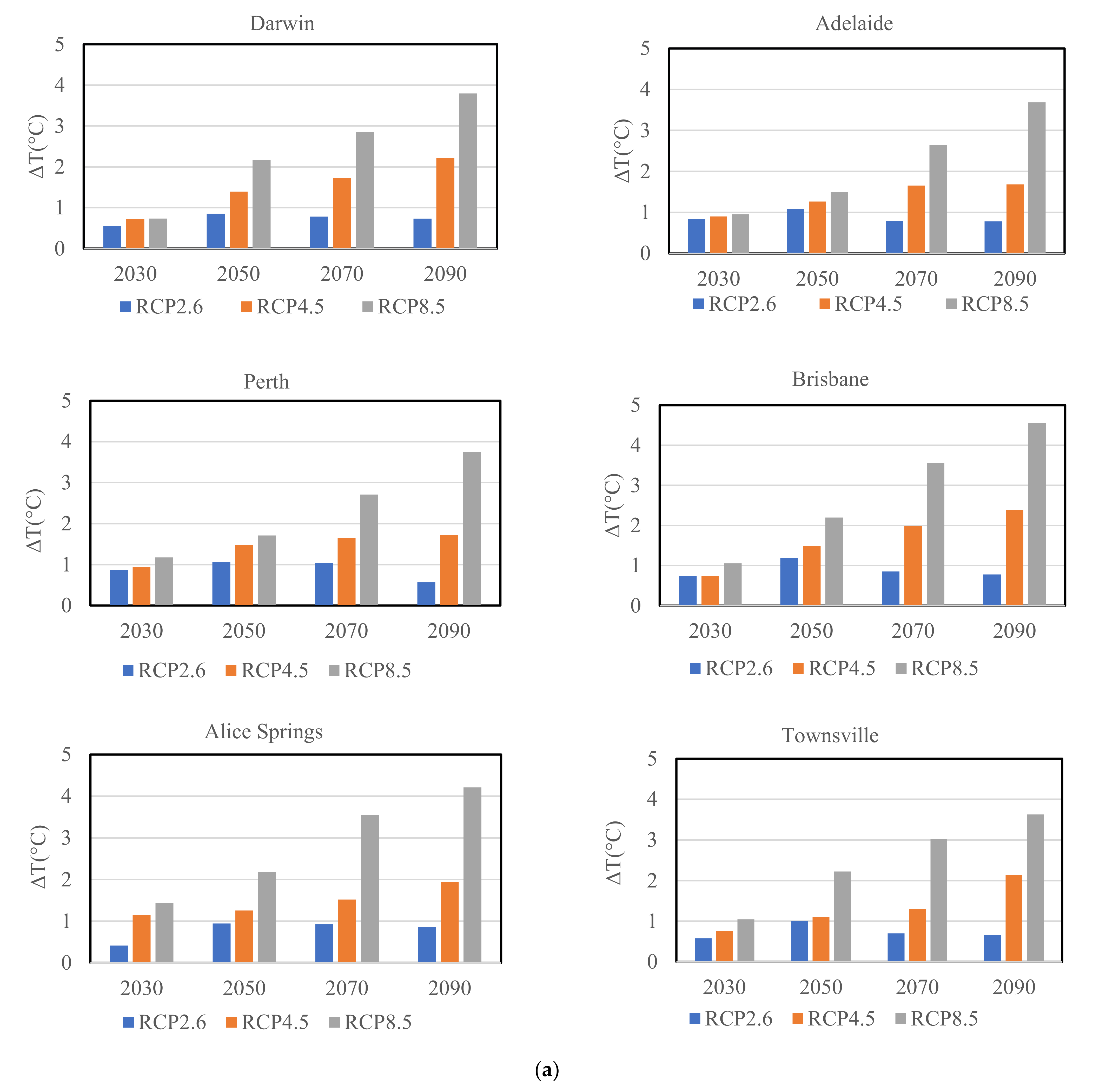
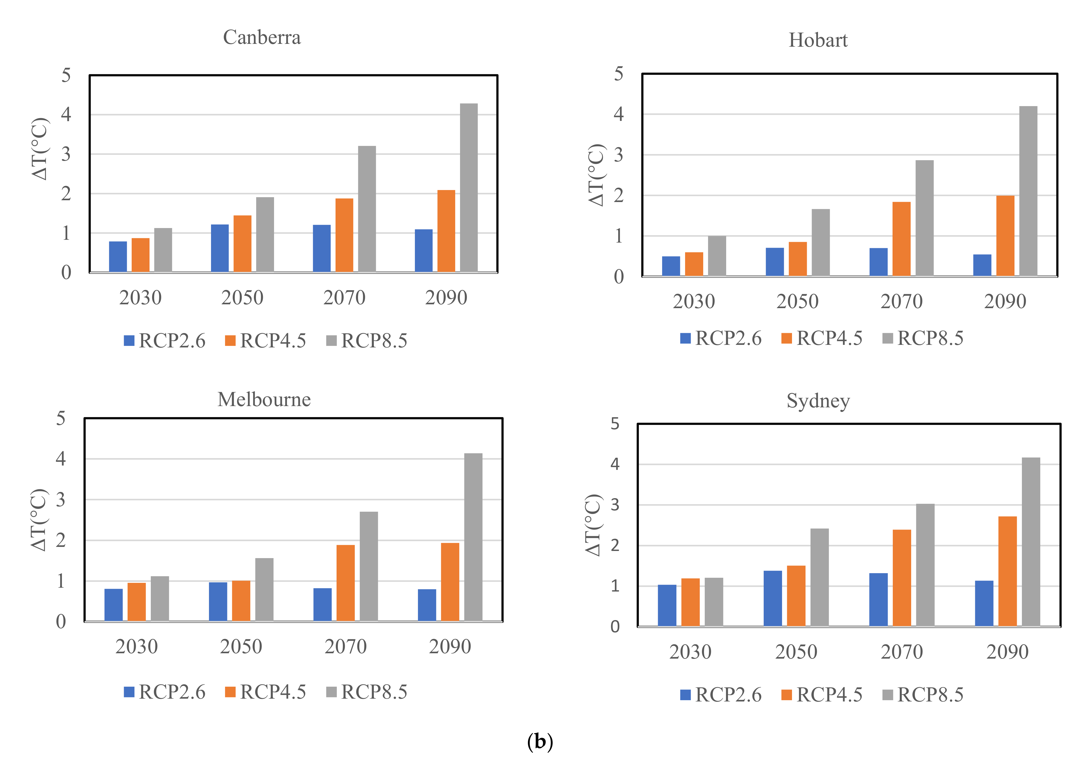
3.1. Future Temperatures

The projected temperature differences for the ten climate zones are given in Figure 4a,b. The temperature steadily rises with time under the RCP4.5 and RCP 8.5 conditions. For RCP2.6, the peak temperatures appear in the 2050s and 2070s for all climate zones. The projected temperatures were greater than 4 °C for RCP8.5 in the 2090s in Brisbane, Sydney, Canberra, Melbourne, and Hobart, which are on the east coast. In contrast, slower temperature rises were seen in most of the western cities, other than Alice Springs. This implies that the east coast regions are significantly affected by the severe carbon emission scenario of RCP8.5.

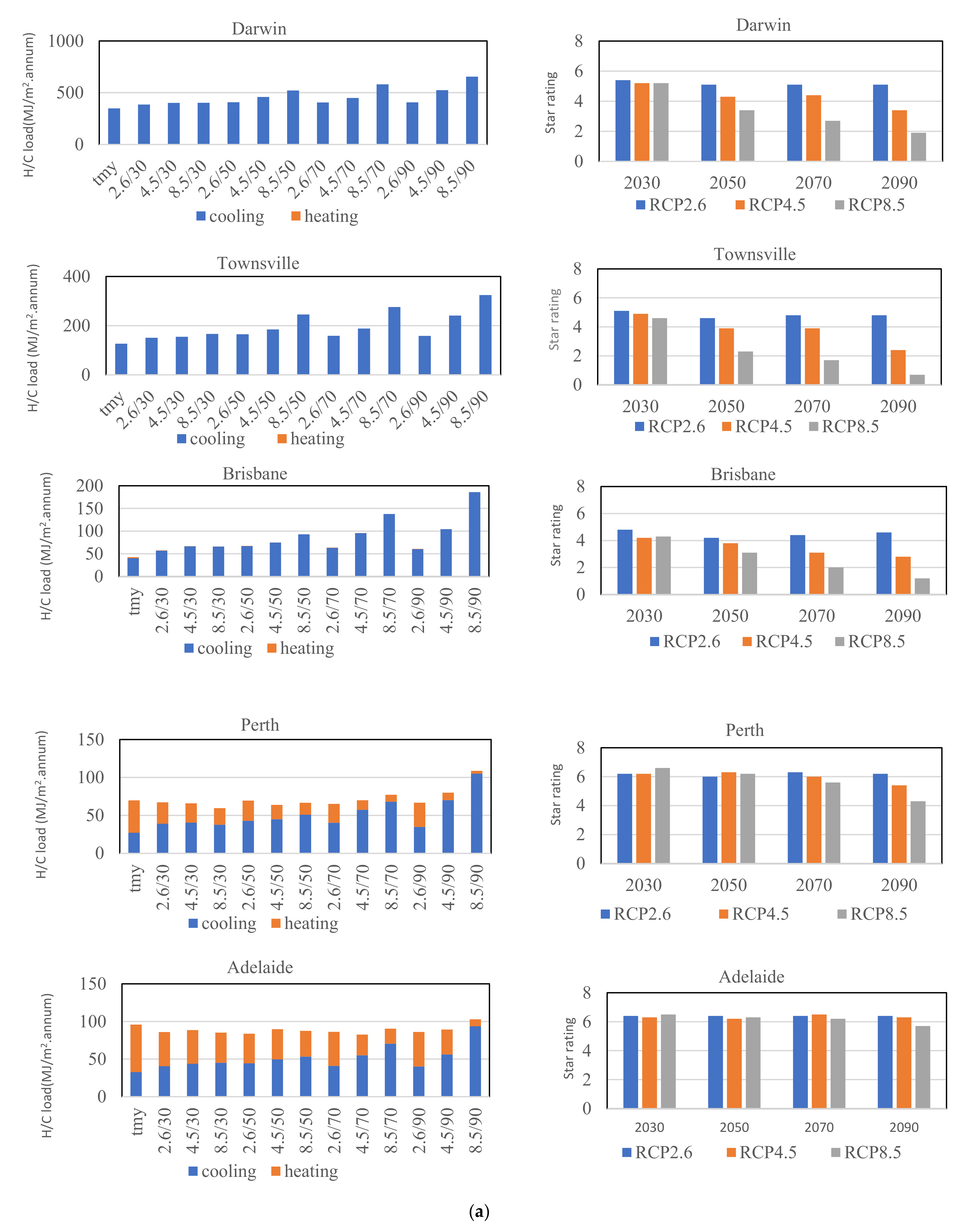
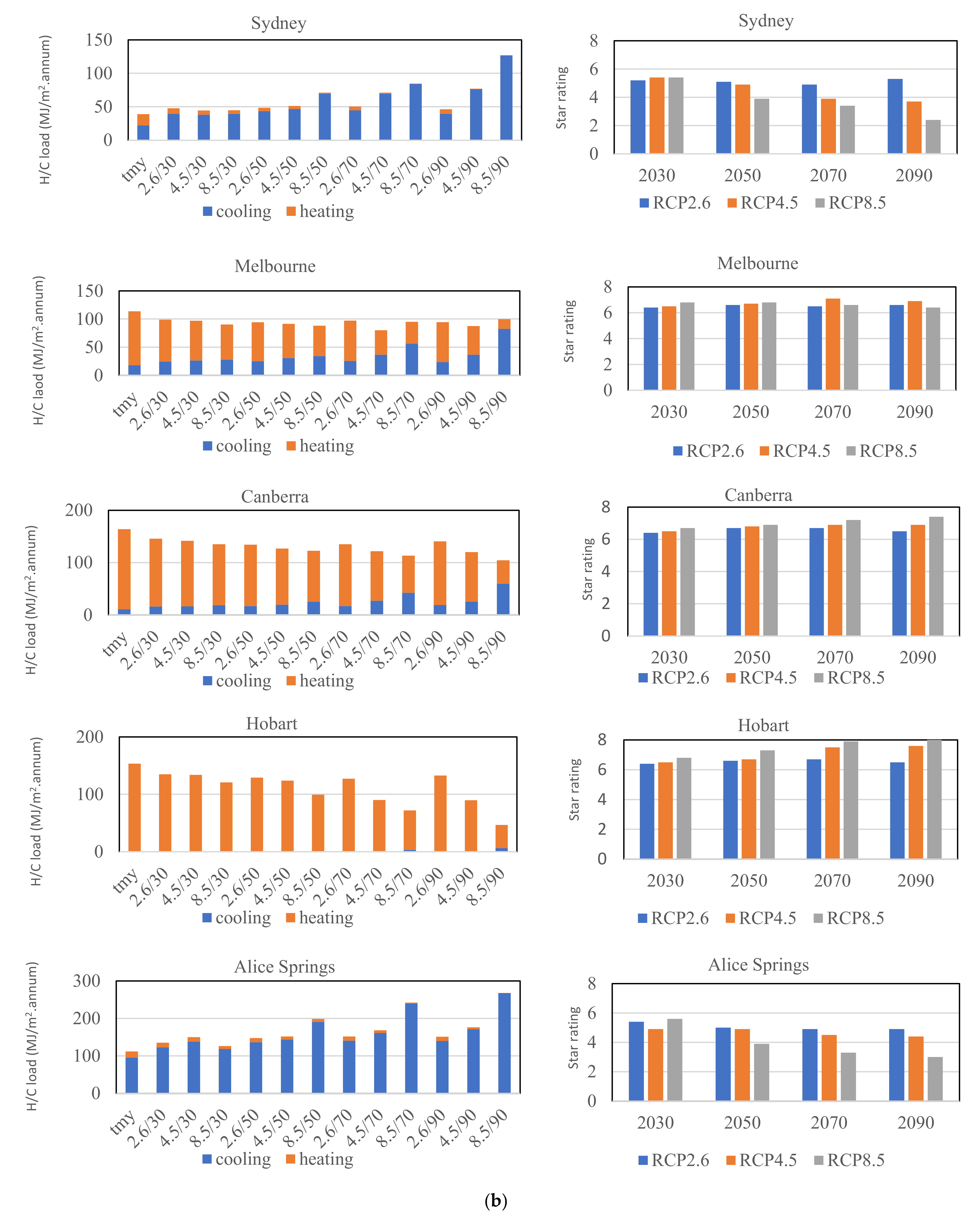
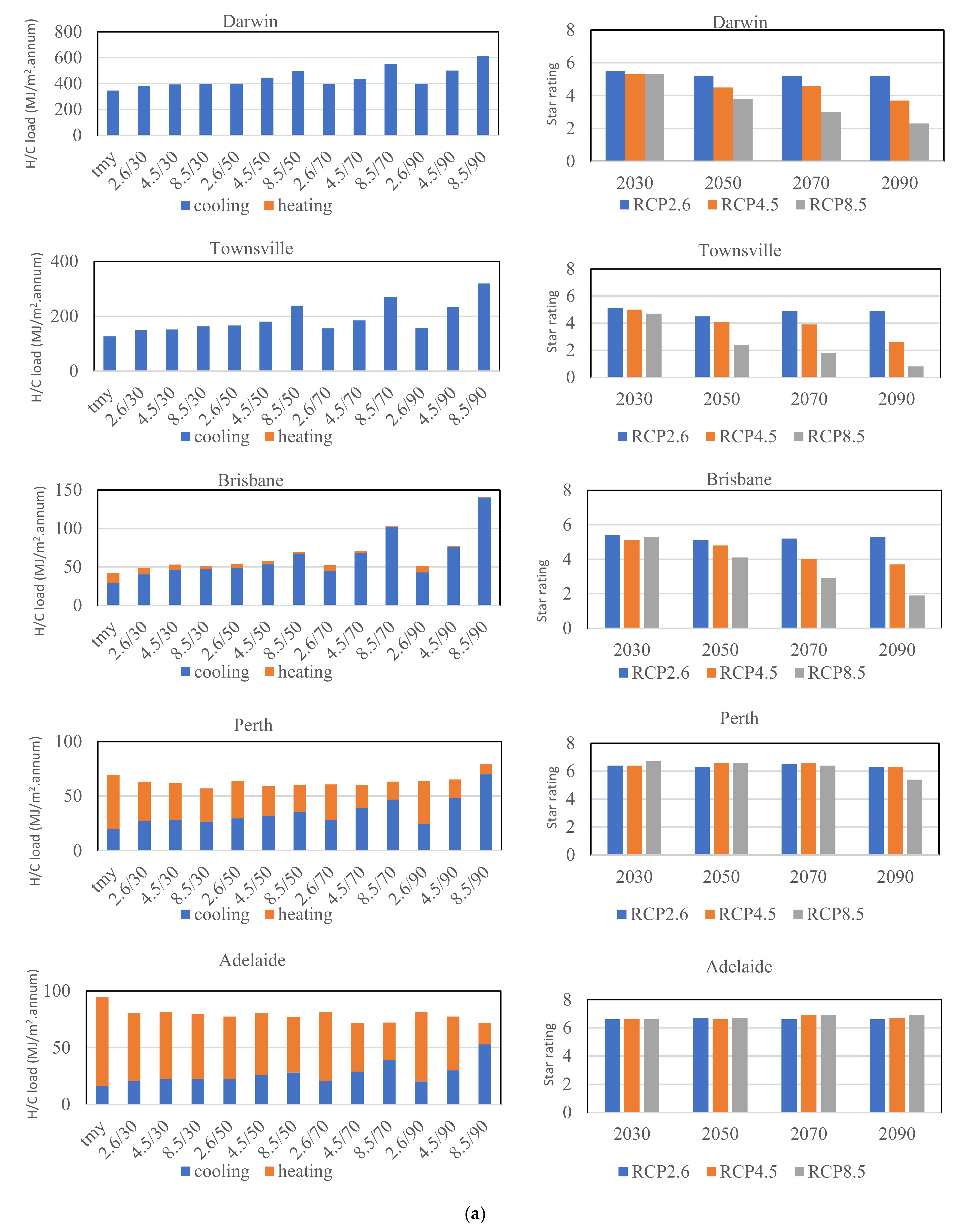
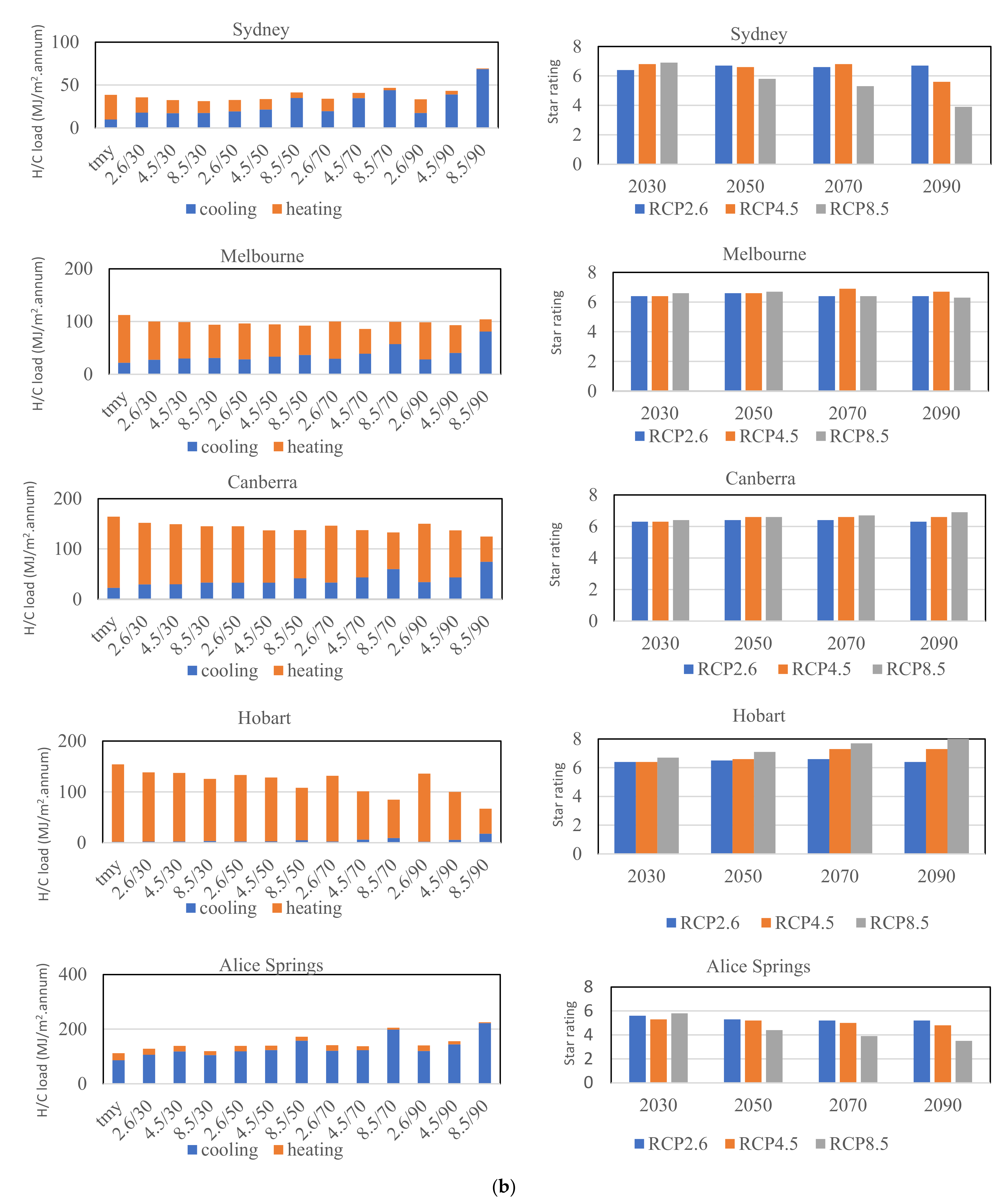
3.2. Space H/C Energy Requirements and Star Ratings in the Future (2030–2100)

Using the predicted future weather files, the H/C energy requirements of the two 6-star houses were calculated using AccuRate for the ten cities, under the three scenarios (RCPs 2.6, 4.5, and 8.5), over the four periods (the 2030s, 2050s, 2070s, and 2090s); this gave a total of 240 simulations in this study. The results for the space H/C requirements are shown in Figure 5 and Figure 6. As expected, the energy requirement will decrease for space heating and increase for space cooling with climate change in all scenarios. For houses in tropical regions such as Darwin and Townsville, space heating is not required in the current and future climates. Under the low emission scenario of RCP2.6, the energy requirements for space cooling in Darwin will increase by around 17% and 15% by the 2070s (with around 50 years of the lifespan of housing) for Houses 1 and 2, respectively (

Table 6. The projected percentage change (%) relative to TMY in annual cooling energy requirements for 6-star houses in ten climate zones.

Location	Periods	House 1			House 2
		RCP2.6	RCP4.5	RCP8.5	RCP2.6	RCP4.5	RCP8.5
Darwin	2030s	10.7	15.3	15.6	9.6	13.5	14.4
	2050s	17.2	31.8	49.8	15.3	28.6	43.3
	2070s	16.6	29.0	66.9	14.8	26.5	59.1
	2090s	16.8	50.8	88.2	14.8	44.5	77.5
Alice Springs	2030s	28.4	44.6	24.1	23.5	37.4	22.1
	2050s	42.9	50.1	99.8	38.0	43.2	83.5
	2070s	47.2	68.6	151.2	40.6	43.1	130.6
	2090s	46.2	79.4	179.9	39.5	68.0	158.4
Townsville	2030s	19.1	22.3	31.3	17.7	20.0	28.6
	2050s	30.2	45.7	93.9	31.4	42.4	88.2
	2070s	25.4	48.5	117.7	23.1	45.8	112.7
	2090s	24.9	90.3	156.1	23.3	84.9	152.3
Brisbane	2030s	40.9	64.8	63.3	39.1	59.2	63.3
	2050s	66.5	85.6	130.5	67.1	84.4	132.9
	2070s	56.3	137.0	241.4	53.6	134.6	254.0
	2090s	49.6	159.1	361.3	48.4	161.9	385.1
Sydney	2030s	77.0	71.6	77.9	81.6	75.5	77.6
	2050s	95.0	110.8	213.1	96.9	118.4	255.1
	2070s	100.5	213.1	279.3	100.0	254.1	348.0
	2090s	77.0	242.8	470.7	77.6	298.0	600.0
Perth	2030s	43.9	49.1	39.1	35.2	40.2	33.2
	2050s	57.9	65.7	87.5	48.2	59.3	78.9
	2070s	48.7	111.4	150.9	40.2	97.0	135.2
	2090s	28.0	158.7	287.1	21.1	141.2	251.3
Canberra	2030s	44.1	45.9	67.6	29.5	30.8	45.8
	2050s	53.2	75.7	128.8	44.5	44.9	82.8
	2070s	53.2	143.2	282.0	45.8	90.3	164.3
	2090s	69.4	127.0	436.9	49.8	91.2	228.2
Adelaide	2030s	23.9	33.6	37.9	26.7	37.9	41.0
	2050s	35.8	51.7	62.7	40.4	60.2	74.5
	2070s	25.4	68.2	115.3	29.8	80.1	144.1
	2090s	22.6	71.9	186.2	26.1	87.0	228.6
Melbourne	2030s	34.4	46.7	54.4	26.1	36.7	42.2
	2050s	39.4	70.0	90.0	29.4	52.3	67.4
	2070s	42.2	103.3	211.1	34.9	78.9	161.9
	2090s	30.0	103.3	358.3	28.4	85.8	271.1
Hobart	2030s	100.0	100.0	200.0	22.2	33.3	77.8
	2050s	100.0	200.0	400.0	38.9	50.0	172.2
	2070s	50.0	550.0	1550.0	27.8	227.8	411.1
	2090s	50.0	450.0	3000.0	11.1	205.6	883.3

). The energy rating is predicted to drop by 0.9 stars (from 6 to 5.1 stars; see

Table 7. Projected star ratings for 6-star House 1 in ten climate zones.

	RCP2.6				RCP4.5				RCP8.5
	2030s	2050s	2070s	2090s	2030s	2050s	2070s	2090s	2030s	2050s	2070s	2090s
Darwin	5.4	5.1	5.1	5.1	5.2	4.3	4.4	3.4	5.2	3.4	2.7	1.9
Alice Springs	5.4	5	4.9	4.9	4.9	4.9	4.5	4.4	5.6	3.9	3.3	3
Townsville	5.1	4.6	4.8	4.8	4.9	3.9	3.9	2.4	4.6	2.3	1.7	0.7
Brisbane	4.8	4.2	4.4	4.6	4.2	3.8	3.1	2.8	4.3	3.1	2	1.2
Perth	6.2	6	6.3	6.2	6.2	6.3	6	5.4	6.6	6.2	5.6	4.3
Sydney	5.2	5.1	4.9	5.3	5.4	4.9	3.9	3.7	5.4	3.9	3.4	2.4
Adelaide	6.4	6.4	6.4	6.4	6.3	6.2	6.5	6.3	6.5	6.3	6.2	5.7
Melbourne	6.4	6.6	6.4	6.4	6.4	6.6	6.9	6.7	6.6	6.7	6.4	6.3
Canberra	6.3	6.4	6.4	6.3	6.3	6.6	6.6	6.6	6.4	6.6	6.7	6.9
Hobart	6.4	6.6	6.7	6.5	6.5	6.7	7.5	7.6	6.8	7.3	7.9	8.6

) for House 1 and 0.8 stars (from 6 to 5.2 stars; see

Table 8. Projected star ratings for 6-star House 2 in ten climate zones.

	RCP2.6				RCP4.5				RCP8.5
	2030s	2050s	2070s	2090s	2030s	2050s	2070s	2090s	2030s	2050s	2070s	2090s
Darwin	5.5	5.2	5.2	5.2	5.3	4.5	4.6	3.7	5.3	3.8	3	2.3
Alice Springs	5.6	5.3	5.2	5.2	5.3	5.2	5	4.8	5.8	4.4	3.9	3.5
Townsville	5.1	4.5	4.9	4.9	5	4.1	3.9	2.6	4.7	2.4	1.8	0.8
Brisbane	5.4	5.1	5.2	5.3	5.1	4.8	4	3.7	5.3	4.1	2.9	1.9
Perth	6.4	6.3	6.5	6.3	6.4	6.6	6.6	6.3	6.7	6.6	6.4	5.4
Sydney	6.4	6.7	6.6	6.7	6.8	6.6	6.8	5.6	6.9	5.8	5.3	3.9
Adelaide	6.6	6.7	6.6	6.6	6.6	6.6	6.9	6.7	6.6	6.7	6.9	6.9
Melbourne	6.4	6.6	6.4	6.4	6.4	6.6	6.9	6.7	6.6	6.7	6.4	6.3
Canberra	6.3	6.4	6.4	6.3	6.3	6.6	6.6	6.6	6.4	6.6	6.7	6.9
Hobart	6.4	6.5	6.6	6.4	6.4	6.6	7.3	7.3	6.7	7.1	7.7	8.1

) for House 2. For the same period under RCP2.6 in Townsville, the space cooling requirement could increase by around 25% and 23% for Houses 1 and 2, respectively. The energy rating for House 1 is projected to drop 1.2 stars for House 1 and 1.1 stars for House 2. Under the highest emission scenario of RCP8.5 by the 2070s, the energy requirements for space cooling in Darwin may increase by around 67% and 59% for Houses 1 and 2, respectively. The energy rating is projected to drop 3.3 stars for House 1 and 3 stars for House 2. For the same period under RCP8.5 in Townsville, the space cooling requirement is projected to increase by around 118% and 113% for Houses 1 and 2, respectively. The star rating could drop 4.3 stars for House 1 and 4.2 stars for House 2. This is a significant challenge facing building design and operations in this scenario.

In subtropical regions such as Alice Springs, which experiences a subtropical hot desert climate (Köppen BWh), for both Houses 1 and 2, there were low energy requirements (16.2 MJ/m².annum for House 1 and 25.9 MJ/m².annum for House 2) for space heating under current (TMY) weather conditions (refer to Figure 4 and Figure 5). Under RCP2.6, the energy requirements for space cooling are projected to increase by around 47% and 41% by 2070 for Houses 1 and 2, respectively. Under RCP8.5 conditions, the corresponding increases will be around 151% and 131%. In terms of star ratings based on the total energy requirement for space heating and cooling, the given star rating represents the energy requirements for housing air conditioning to achieve thermal comfort in both winter and summer. Under RCP2.6 conditions, by the 2070s, the energy rating is projected to drop by 1.1 stars and 1.8 stars for Houses 1 and 2, respectively. Under RCP8.5 conditions, by the 2070s, the energy rating is projected to drop by 2.7 stars and 2.1 stars for Houses 1 and 2, respectively. There is a low energy requirement for space heating in both houses under the three RCPs by the 2070s.

Under the Köppen climate classification, both Brisbane and Sydney have a humid subtropical climate (Cfa). For House 1 in Brisbane, there is a low energy requirement (2.2 MJ/m²·annum) for space heating in the current (TMY) climate and no energy requirements for space heating under RCP4.5 by the 2090s and under RCP8.5 by the 2050s. The energy requirements for space cooling are projected to increase by around 56% and 241% by the 2070s under RCP2.6 and RCP8.5, respectively. This could cause a decrease in star rating of 0.6 stars and 4 stars, respectively. For House 2 under the TMY climate, the energy requirements for space heating are 13.6 MJ/m².annum, and space heating will not be required under RCP8.5 by the 2070s. The energy requirements for space cooling are projected to increase by around 52% and 103% by the 2070s under RCP2.6 and RCP8.5 conditions, respectively. This causes an energy-rating decrease of 0.8 stars and 3.1 stars, respectively. Under TMY weather conditions in Sydney, the energy requirement for space H/C is balanced with that for space heating and cooling for House 1 and is dominated by space heating (refer to Figure 5 and Figure 6) for House 2. With the total energy requirements for space heating and cooling, the energy rating will vary with the combined impacts of global warming on space heating and cooling. Under RCP2.6 by the 2070s, the energy requirements for space cooling are projected to increase by around 100% for both Houses 1 and 2 and decrease by 44.5% for space heating in House 1 and 19.6% in House 2. The energy rating could drop by 1.1 stars for House 1 and increase by 0.6 stars for House 2. Under RCP8.5, by the 2070s, space heating will not be required for House 1 and a small amount of energy (2.8 MJ/m².annum) will be required for space heating in House 2. The energy requirements for space cooling are projected to increase by around 85% and 47% for Houses 1 and 2, respectively. The corresponding energy star rating could drop by 2.6 stars and 0.7 stars, respectively.

Both Perth and Adelaide have Köppen climate classifications of Csa. For both Houses 1 and 2 under current (TMY) climates in the two cities, space heating requirements are greater than those for space cooling (Figure 5 and Figure 6). Under RCP 2.6 and 4.5 conditions, by the 2070s, the energy rating is projected to benefit from global warming (i.e., become higher than six stars for both Houses 1 and 2; refer to Table 7 and Table 8, respectively). Under RCP8.5 conditions, by the 2070s in Perth, a low level of energy requirements will be required for House 1’s space heating (9.2 MJ/m²·annum), and a decrease by 78%, and an increase of 151% for space cooling will be required, compared to current (TMY) climate conditions. The energy rating could drop by 0.4 stars. Under RCP8.5 conditions, for House 2 in Perth—and both Houses 1 and 2 in Adelaide—the energy rating will benefit from RCP8.5 conditions, with an increase of up to 0.9 stars by 2070 for House 2 in Adelaide.

Canberra, Melbourne, and Hobart have an oceanic climate with a Köppen climate classification Cfb. Melbourne has a temperate oceanic climate and Hobart has a mild temperate oceanic climate. These cities are heating-dominated regions. Under current TMY and future climates with the three RCPs, there are lower energy requirements for space cooling in Houses 1 and 2 in Hobart. Under RCP8.5 conditions, by the 2090s in Hobart, the energy rating will increase by 2.6 stars and 2.1 stars for Houses 1 and 2, respectively. Under RCP2.6 conditions, by the 2070s, Melbourne and Canberra will still be heating-dominated regions. The energy rating is projected to increase by around 0.5 stars and 0.6 stars for Houses 1 and 2 in Melbourne and Canberra, respectively. Under RCP4.5 conditions, by the 2070s, Melbourne will become a space heating and cooling balanced region. The energy rating is projected to increase by around one star in Melbourne for both Houses 1 and 2. In Canberra, the increase in the energy rating will be 0.9 stars and 0.6 stars for Houses 1 and 2, respectively. Under RCP8.5 conditions, by the 2090s, Melbourne will become a cooling-dominated region, and Canberra will become a space heating and cooling balanced region. The energy rating is projected to increase by around 0.3 stars for both Houses 1 and 2 in Melbourne, and 2.6 stars for House 1 and 0.9 stars for House 2 in Canberra.

4. Discussion

This paper presents an approach to construct future weather files for building energy performance simulation in Australia under three carbon emission scenarios—RCP2.6 (low), 4.5 (medium), and high (8.5)—in the 2030s, 2050s, 2070s, and 2090s. The critical parameters affecting building thermal performance are air temperature, humidity, wind speed, and solar radiation. Using the morphing method to construct the future weather files, the hourly data of the critical variables were developed based on current (TMY) hourly data plus monthly change values, which were derived from downscaling the results of the eight GCMs that were selected based on ranking results from the Climate Framework.

Australia has complex and diverse terrain conditions. Ten cities (climate zones) were selected for the case studies. As expected, the predicted temperature changes with the trends of RCPs. For the ten cities under RCP2.6, the highest increase in temperature will occur around 2050s (Figure 3a,b). Under RCPs 4.5 and 8.5, the temperature will increase from now (baseline) to the 2090s. The temperature changes by 2090s are substantial under RCP8.5 compared to the 2016 TMY baseline. The increase in temperature will be greater than 4 °C in Alice Springs, Brisbane, Canberra, Hobart, Melbourne, and Sydney, and 3–4 °C in the other four cities. The effects of the temperature increase will result in substantial changes to space heating and cooling loads. RCP8.5 shows higher impact on space cooling loads than the lower (RCP2.6) and medium (RCP4.5) scenarios (Table 6).

In this study, although two detached houses, representing around 80% of the housing stock in Australia, were used to analyse the impact of climate change on space H/C loads, not all building types were included in the analysis. Urban heat islands may have a significant impact on building energy performance in urban areas. Unban heat islands were not explicitly modelled in this study. Our future work will consider more residential building types (such as townhouses, apartments, etc.) and urban heat islands for the other regions of Australia.

5. Conclusions

Using the methodology of morphing, the weather files were constructed based on the 2016 TMY data and predicted data generated from eight GCMs for three representative concentration pathways (RCP2.6, RCP4.5, and RCP8.5) from 2020 to 2100. The future temperature for the ten selected representative cities is projected to increase no more than 1.5 °C, 3 °C, and 4.5 °C by the 2090s under the RCP2.6, 4.5, and 8.6 conditions, respectively. The impact of climate change on building energy performance varies with climate region. In this study, two typical houses (House 1—large size and House 2—medium size) were selected to evaluate the impacts of climate change in different regions.

In tropical regions (such as Darwin and Townsville), space heating will not be required, and space cooling will increase with global warming. Under RCP2.6 conditions, by the 2070s (around 50-year lifespan houses), space cooling is projected to increase by around 16% and 24% in Darwin and Townville, respectively. The energy rating will drop from six stars to 5.2 stars and 4.9 stars, respectively. Under RCP8.5 conditions, by the 2070s, space cooling is projected to increase by around 60% and 115% in Darwin and Townsville, respectively. The star rating will drop from six stars to 2.7 stars and 1.7 stars, respectively. This will significantly increase the energy required for space cooling. This is a considerable challenge facing building design and operation.

In subtropical regions such as Alice Springs and Brisbane, under current (TMY) climates, low energy requirements are placed on space heating. These energy ratings will drop with global warming. Under RCP2.6 conditions, by the 2070s, the energy rating is projected to drop from six stars to 4.9 stars and 4.2 stars for Houses 1 and 2 in Alice Springs, respectively. The energy rating in Brisbane will drop from six stars to 4.4 stars and 5.2 stars, respectively. Under RCP8.5 conditions, by the 2090s, the energy requirements for space heating in Alice Springs will become negligible (at less than 1 MJ/m²·annum). This will occur in Brisbane—for House 1—under all three RCPs and for House 2 under RCP8.5 conditions by the 2070s. Under current (TMY) climates in Sydney, the energy requirement for space H/C is balanced with space heating and cooling for House 1 and dominated by space cooling for House 2. In Sydney, the energy requirements for space heating of House 1 can be ignored under RCP4.5 conditions by the 2090s and under RCP8.5 conditions by the 2070s, and under RCP8.5 conditions by the 2090s for House 2.

In oceanic climate regions (Köppen Cfb) such as Melbourne, Canberra, and Hobart, the energy requirements for thermal comfort under current (TMY) climates are dominated by space heating. The case study herein shows that there is a very low energy demand for space cooling in Hobart under current or future climates under all three RCPs. As global warming is beneficial to space heating, under RCP8.5 conditions, by the 2090s, the energy rating is projected to increase from six stars to 8.6 stars and 8.1 stars for Houses 1 and 2 in Hobart, respectively. Under RCP2.6 conditions, by the 2070s, Melbourne and Canberra will still be heating-dominated regions. Under RCP4.5, conditions by the 2070s, Melbourne will become a heating and cooling balanced region. Under RCP8.5 conditions, by the 2090s, Melbourne will become a cooling-dominated region, and Canberra will become a heating and cooling balanced region. The energy rating is projected to increase from six stars to 8.6 stars in Canberra.

Both Perth and Adelaide have Mediterranean climates (Köppen Csa). Under current (TMY) climates in the two cities, the energy requirements for space heating are greater than those for space cooling. For House 1, under RCP2.6 conditions, by the 2030s, both Perth and Adelaide are projected to become space heating and cooling balanced. House 2 is projected to become space heating and cooling balanced in Perth by the 2050s under RCP4.5 conditions, and in Adelaide by the 2070s under RCP8.6 conditions. In general, the change in the energy rating will be smaller than one star for both Houses 1 and 2 in the two cities under the three RCPs by the 2100s.

References

1. COAG Energy Council. Report for Achieving Low Energy Homes 2018. Available online: https://www.energy.gov.au/publications/report-achieving-low-energy-existing-homes (accessed on 25 June 2021).
2. King, A.; Karoly, D.; Henley, B. Australian climate extremes at 1.5 °C and 2 °C of global warming. Nat. Clim. Chang. 2017, 7, 412–416. [Google Scholar] [CrossRef]
3. Ren, Z.; Chen, D.; James, M. Evaluation of a whole-house energy simulation tool against measured data. Energy Build. 2018, 171, 116–130. [Google Scholar] [CrossRef]
4. National Construction Code 2019. Building Code of Australia, Volume 1. Australian Building Codes Board. Available online: http://www.abcb.gov.au (accessed on 25 June 2021).
5. IPCC AR5 Synthesis Report. Climate Change 2014. Available online: http://www.ipcc.ch/report/ar5/ (accessed on 25 June 2021).
6. Van Vuuren, D.P.; Edmonds, J.; Kainuma, M.; Riahi, K.; Thomson, A.; Hibbard, K.; Hurtt, G.C.; Kram, T.; Krey, V.; Lamarque, J.F.; et al. The representative concentration pathways: An overview. Clim. Chang. 2011, 109, 5–31. [Google Scholar] [CrossRef]
7. Xu, P.; Huang, Y.J.; Miller, N.; Schlegel, N.; Shen, P. Impacts of climate change on building heating and cooling energy patterns in California. Energy 2012, 44, 792–804. [Google Scholar] [CrossRef]
8. Shen, P. Impacts of climate change on U.S. building energy use by using downscaled hourly future weather data. Energy Build. 2017, 134, 61–70. [Google Scholar] [CrossRef]
9. Invidiata, A.; Ghisi, E. Impact of climate change on heating and cooling energy demand in houses in Brazil. Energy Build. 2016, 130, 20–32. [Google Scholar] [CrossRef]
10. Kalvelage, K.; Passe, U.; Rabideau, S.; Takle, E.S. Changing climate: The effects on energy demand and human comfort. Energy Build. 2014, 76, 373–380. [Google Scholar] [CrossRef]
11. Wang, X.; Chen, D.; Ren, Z. Assessment of climate change impact on residential building heating and cooling energy requirement in Australia. Build. Environ. 2010, 45, 1663–1682. [Google Scholar] [CrossRef]
12. Belcher, S.; Hacker, J.; Powell, D. Constructing design weather data for future climates. Build. Serv. Eng. Res. Technol. 2005, 26, 49–61. [Google Scholar] [CrossRef]
13. Wang, H.; Chen, Q. Impact of climate change heating and cooling energy use in buildings in the United States. Energy Build. 2014, 82, 428–436. [Google Scholar] [CrossRef] [Green Version]
14. Ren, Z.; Paevere, P.; Chen, D. Feasibility of off-grid housing under current and future climates. Appl. Energy 2019, 241, 196–211. [Google Scholar] [CrossRef]
15. Flores-Larsen, S.; Filippin, C.; Barea, G. Impact of climate change on energy use and bioclimatic design of residential buildings in the 21st century in Argentina. Energy Build. 2019, 184, 216–229. [Google Scholar] [CrossRef]
16. Wang, L.; Liu, X.; Brown, H. Prediction of the impacts of climate change on energy consumption for a medium-size office building with two climate models. Energy Build. 2017, 157, 218–226. [Google Scholar] [CrossRef]
17. Arima, Y.; Ooka, R.; Kikumoto, H.; Yamanaka, T. Effect of climate change on building cooling loads in Tokyo in the summers of the 2030s using dynamically downscaled GCM data. Energy Build. 2016, 114, 123–129. [Google Scholar] [CrossRef]
18. Sabunas, A.; Kanapickas, A. Estimation of climate change impact on energy consumption in a residential building in Kaunas, Lithuania, using HEED Software. Energy Procedia 2017, 128, 92–99. [Google Scholar] [CrossRef]
19. Frank, T. Climate change impacts on building heating and cooling energy demand in Switzerland. Energy Build. 2005, 37, 1175–1185. [Google Scholar] [CrossRef]
20. Liu, Y.; Stouffs, R.; Tablada, A.; Wong, N.H.; Zhang, J. Comparing micro-scale weather data to building energy consumption in Singapore. Energy Build. 2017, 152, 776–791. [Google Scholar] [CrossRef]
21. Pérez-Andreu, V.; Aparicio-Fernández, C.; Martínez-Ibernón, A.; Vivancos, J.L. Impact of climate change on heating and cooling energy demand in a residential building in a Mediterranean climate. Energy 2018, 165, 63–74. [Google Scholar] [CrossRef]
22. Hekkenberg, M.; Moll, H.; Uiterkamp, S. Dynamic temperature dependence patterns in future energy demand models in the context of climate change. Energy 2009, 34, 1797–1806. [Google Scholar] [CrossRef]
23. Seljom, P.; Rosenberg, E.; Fidje, A.; Haugen, J.; Meir, M.; Rekstad, J.; Jarlset, T. Modelling the effects of climate change on the energy system—A case study of Norway. Energy Policy 2011, 39, 7310–7321. [Google Scholar] [CrossRef]
24. Zhu, M.; Pan, Y.; Huang, Z.; Xu, P. An alternative method to predict future weather data for building energy demand simulation under global climate change. Energy Build. 2016, 113, 74–86. [Google Scholar] [CrossRef]
25. Ma, Q.; Yang, H.; Zhang, C.; Peng, Z. Effects of global warming for building energy demand in China. Comput. Model. New Technol. 2014, 4, 3–7. [Google Scholar]
26. Pretlove, S.; Oreszczyn, T. Climate change: Impact on the environmental design of buildings. Build. Serv. Eng. Res. Technol. 1998, 19, 55–58. [Google Scholar] [CrossRef]
27. Cartalis, C.; Synodinou, A.; Proedrou, M.; Tsangrassoulis, A.; Santamouris, M. Modifications in energy demand in urban areas as a result of climate changes: An assessment for the southeast Mediterranean region. Energy Conversat. Manag. 2001, 42, 1647–1656. [Google Scholar] [CrossRef]
28. Akpinar-Ferrand, E.; Singh, A. Modelling increased demand of energy for air conditioners and consequent CO2 emissions to minimize health risks due to climate change in India. Environ. Sci. Policy 2010, 13, 702–712. [Google Scholar] [CrossRef]
29. Pyrgou, A.; Castaldo, V.; Pisello, A.; Cotana, F.; Santamouris, M. Differentiating responses of weather files and local climate change to explain variations in building thermal-energy performance simulations. Solar Energy 2017, 153, 224–237. [Google Scholar] [CrossRef]
30. Pisello, A.; Pignatta, G.; Castaldo, V.; Cotana, F. The impact of local microclimate boundary conditions on building energy performance. Sustainability 2015, 7, 9207–9230. [Google Scholar] [CrossRef] [Green Version]
31. Waddicor, D.; Fuentes, E.; Sisó, L.; Salom, J.; Favre, B.; Jiménez, C.; Azar, M. Climate change and building ageing impact on building energy performance and mitigation measures application: A case study in Turin, northern Italy. Build. Environ. 2016, 102, 13–25. [Google Scholar] [CrossRef]
32. Roshan, G.; Orosa, J.; Nasrabadi, T. Simulation of climate change impact on energy consumption in buildings, case study of Iran. Energy Policy 2012, 49, 731–739. [Google Scholar] [CrossRef]
33. Dirks, J.; Gorrissen, W.; Hathaway, J.; Skorski, D.; Scott, M.; Pulsipher, T.; Huang, M.; Liu, Y.; Rice, J. Impacts of climate change on energy consumption and peak demand in buildings: A detailed regional approach. Energy 2015, 79, 20–32. [Google Scholar] [CrossRef] [Green Version]
34. Nateghi, R.; Mukherjee, S. A multi-paradigm framework to assess the impacts of climate change on end-use energy demand. PLoS ONE 2017, 12, e0188033. [Google Scholar] [CrossRef] [PubMed] [Green Version]
35. Mendoza, D.; Bianchi, C.; Thomas, J.; Ghaemi, Z. Modelling county-level energy demands for commercial buildings due to climate variability with prototype building simulation. World 2020, 1, 7. [Google Scholar] [CrossRef]
36. Bianchi, C.; Mendoza, D.; Didier, R.; Thomas, T.; Smith, A. Energy demands for commercial buildings with climate variability based on emission scenarios. In Proceedings of the ASHRAE 2017 Winter Conference, Las Vegas, NV, USA, 28 January–1 February 2017. [Google Scholar]
37. Kikumoto, H.; Ooka, R.; Arima, Y.; Yamanaka, T. Study on the future weather data considering the global and local climate change for building energy simulation. Sustain. Cities Soc. 2015, 14, 404–413. [Google Scholar] [CrossRef]
38. Chan, A. Developing future hourly weather files for studying the impact of climate change on building energy performance in Hong Kong. Energy Build. 2011, 43, 2860–2868. [Google Scholar] [CrossRef]
39. Whetton, P.; Hennessy, K.; Clarke, J.; McInnes, K.; Kent, D. Use of Representative Climate Futures in impact and adaptation assessment. Clim. Chang. 2012, 115, 433–442. [Google Scholar] [CrossRef]
40. Clarke, J.; Whetton, P.; Hennessy, K. Providing application-specific climate projections datasets: CSIRO’s Climate Futures Framework. In Proceedings of the 19th International Congress on Modelling and Simulation, Perth, WA, Australia, 12–16 December 2011. [Google Scholar]
41. The Climate Future Framework. Available online: https://www.climatechangeinaustralia.gov.au/en/projections-tools/climate-futures-tool/projections/ (accessed on 25 May 2021).
42. Liley, B. Creation of 2016 NatHERS Reference Meteorological Years; NIWA Client Report No. 2017103WN, Prepared for Australian Government Department of Environment and Energy; Nationwide House Energy Rating Scheme: Canberra, ACT, Australia, 2017. [Google Scholar]
43. Nakicenovic, N.; Swart, R. Emission Scenarios -Special Report of the Intergovernmental Panel on Climate Change; Cambridge University Press: Cambridge, UK, 2000. [Google Scholar]
44. Nationwide House Energy Rating Scheme (NatHERS). Available online: http://www.nathers.gov.au (accessed on 25 May 2021).
45. Köppen Climate Classification System. Available online: https://en.wikipedia.org/wiki/köppen_climate_classification (accessed on 16 June 2021).
46. Climate Change in Australia. Available online: http://www.climatechangeinaustralia.gov.au/en/ (accessed on 25 June 2021).
47. Walsh, P.; Delsante, A. Calculation of the thermal behaviour of multi-zone buildings. Energy Build. 1983, 5, 231–242. [Google Scholar] [CrossRef]
48. Ren, Z.; Chen, D. Enhanced air flow modelling for AccuRate—A nationwide house energy rating tool. Build. Environ. 1983, 45, 1276–1286. [Google Scholar] [CrossRef]
49. NatHERS National Administrator. Nationwide House Energy Rating Scheme (NatHERS)—Software Accreditation Protocol; NatHERS National Administrator: Canberra, ACT, Australia, 2012. [Google Scholar]
50. House Energy Rating. Available online: https://en.wikipedia.org/wiki/House_Energy_Rating (accessed on 25 June 2021).
Figure 1. Climate future ‘matrices’ for Melbourne in RCP8.5 2090 [46].
Energies 14 04805 g001
Figure 2. Ranking of multi-variate variables.
Energies 14 04805 g002
Figure 3. The floor plans of House 1 (a) and House 2 (b).
Energies 14 04805 g003
Figure 4. (a) Projections of the temperature change in degrees Celsius (°C) in six Australian cities under the three RCPs (2.6, 4.5, and 8.5). (b) Projections of the temperature change in degrees Celsius (°C) in the other four Australian cities under the three RCPs (2.6, 4.5, and 8.5).
Energies 14 04805 g004aEnergies 14 04805 g004b
Figure 5. (a) H/C energy consumption and star ratings in TMY and the future weather for House 1 in five cities. (b) H/C energy consumption and star ratings in TMY and the future weather for House 1 in the other five cities.
Energies 14 04805 g005aEnergies 14 04805 g005b
Figure 6. (a) H/C energy consumption and star ratings in TMY and the future weather for House 2 in five cities. (b) H/C energy consumption and star ratings in TMY and the future weather for House 1 in the other five cities.
Energies 14 04805 g006aEnergies 14 04805 g006b