Article

Outlier Detection in Buildings’ Power Consumption Data Using Forecast Error

1
Univ. Grenoble Alpes, CNRS, Grenoble INP, G2Elab, F-38000 Grenoble, France
2
Department of Electrical and Electronic Engineering, Universidade Federal de Santa Catarina, Florianópolis 88040-900, Brazil
*
Author to whom correspondence should be addressed.
Energies 2021, 14(24), 8325; https://doi.org/10.3390/en14248325
Submission received: 28 November 2021 / Revised: 7 December 2021 / Accepted: 8 December 2021 / Published: 10 December 2021
(This article belongs to the Special Issue Energy Management for Smart Buildings)

Abstract

:
Buildings play a central role in energy transition, as they were responsible for 67.8% of the total consumption of electricity in France in 2017. Because of that, detecting anomalies (outliers) is crucial in order to identify both potential opportunities to reduce energy consumption and malfunctioning of the metering system. This work aims to compare the performance of several outlier detection methods, such as classical statistical methods (as boxplots) applied to the actual measurements and to the difference between the measurements and their predictions, in the task of detecting outliers in the power consumption data of a tertiary building located in France. The results show that the combination of a regression method, such as random forest, and the adjusted boxplot outlier detection method have promising potential in detecting this type of data quality problem in electricity consumption.

1. Introduction

The energy consumed in buildings accounts for a significant share of global energy consumption. In France, according to Bilan RTE 2018 [1], approximately 67.8% of electricity is consumed in buildings, both residential and tertiary. These figures indicate that buildings play a central role in energy transition.
The increased use of intermittent renewable energy sources, such as solar energy, makes the use of machine learning methods combined with demand side management more and more frequent. For example, the anomaly detection using machine-learning techniques can help to identify unusual energy consumption of assets [2,3,4] and detect equipment faults [5].
Several methods for the detection of outliers have been used in recent times. Classic statistical methods, such as the three-sigma rule [6] and the boxplot method [7], have been highly used. However, these techniques assume a symmetrical data distribution and the performance of these techniques is highly dependent on this feature, which is commonly unknown for power consumption data.
To work around the issue of unknown data distribution, researchers have used regression-based methods to tackle this problem. The first step, called the training phase, comprises the definition of a regression model that fits the data. After the construction of the model, every data sample is compared with the model instances in the test phase [8]. A data point is labeled as an outlier if a remarkable deviation occurs between the actual value and its expected value produced by the regression model [9]. Several techniques were used to detect outliers using regression methods. For example, in [10] the author used linear regression to detect outliers and in [11] an auto regressive moving average (ARMA) was used as the regression technique.
Therefore, this work aims at the application of a hybrid method, combining regression techniques and classical statistic outlier methods focusing on detecting outliers of a dataset that contains measurements of electrical energy consumption of a tertiary building. The random forest [12] method as a regression technique to construct a model was used in this work. Afterward, all measured samples were compared with the model instances, resulting in an error. The statistical outlier detection methods were then implemented to search high error values in order to classify them as potential outliers. This combination is called the forecast error method.
The construction of a predictive model of energy consumption in a building can be of great importance for energy managers. Through these models, it is possible to plan from the short term optimization of energy consumption costs to the allocation of assets in case of preventive maintenance with low impact on the building’s normal activity. In addition, the implementation of an algorithm that can detect anomalies integrated into a building management system can facilitate the identification of potential energy consumption reduction or even the need to perform corrective maintenance on an asset that may present a defect in real time.
The following section exposes the statistical outlier detection methods employed in this work. Afterward, the regression (forecast) method employed and the error metrics that can be used to assess the performance of this method are briefly introduced. The combination of these techniques is applied in two datasets. In the first one, called “adapted data”, twelve outliers were manually introduced in healthy synthetic electricity consumption data. The second one consists in “real data” measurements of the electricity consumption, with outliers generated by problems inherent to buildings’ metering systems. The results show that the combination of a regression technique and the adjusted boxplot method [13] presents the better performance compared with the other methods when searching outliers in the tested datasets.

2. Methods for Outlier Detection

An outlier is an observation that deviates so much from other observations as to arouse suspicions that it was generated by a different mechanism [14]. This type of sample can indicate malfunctioning of the metering system or even in a load itself. In addition, if this data quality problem is too persistent it can affect the accuracy of eventual machine-learning algorithms using this dataset. Therefore, its identification and correction are important steps in the data pre-processing.
Standard outlier detection consists of two main components. The first one is calculating an outlier score for every data instance. The outlier score can be the value itself or even the difference between the value and its prediction [15], considering that the prediction model was generated based on healthy data. Other formulations, such as the local outlier factor [16], calculate this score by comparing the value to its k-nearest neighbors in a feature space. The second component is thresholding the outlier scores by the application of some statistical methods. This step decides how highest scoring points are labelled as outliers.
In this work, several statistical methods for thresholding were applied as the three sigma rule [6], the median absolute deviation [17], the original boxplot [7], the skewed boxplot [18] and finally the adjusted boxplot [13]. Each of these methods is detailed in the following sections.

2.1. Three-Sigma Rule

The three-sigma rule is a simple and heuristic method for outlier detection [6]. In a symmetrical distribution, the probability of a sample to be within the range between μ ± 3σ, where μ is the mean and σ is the standard deviation (STD), is 99.7%, as shown in Figure 1.
Therefore, the upper and lower bounds that defines if a value is an outlier or not, can be calculated by applying the following equations in which UPB represents the upper bound and LWB the lower bound. Samples that are higher than the upper bound, or lower than the lower bound, are potential outliers.
U P B = μ + 3 * σ
L W B = μ 3 * σ
Since the three-sigma rule is based on the mean value and the standard deviation, this method is sensitive to the presence of extreme outliers.

2.2. Mean Absolute Deviation (MAD)

Because of its sensitivity to the presence of outliers, the mean value is not the most suitable measure of central tendency to be used in the outlier detection. The median value, another measure of central tendency, is more adapted to this task due to its insensitivity to the existence of outliers in the dataset. The median is defined as the value associated with the mean rank after sorting the data ascendingly.
The median absolute deviation [20] is then defined as the median of the absolute deviation from the median, and can be described as follows:
M A D = b * m e d ( | x i m e d ( X ) | )
In this equation, b is a constant, suggested as 1.4826, x i represents each sample and X is the vector that contains all samples. The upper ( U P B M ) and lower ( L W B M ) bounds can be calculated by the application of the following equations:
U P B M = m e d ( X ) + 3 * M A D
L W B M = m e d ( X ) 3 * M A D

2.3. Boxplot

The modern boxplot, described in more detail by Tukey [7], is a graphical method for detecting potential outliers through a box and whiskers plot with restrictions on the data used [21]. In order to provide a robust measurement of the data series, the boxplot uses some characteristic values of the series, such as the median and the values of the first (25%) and the third (75%) quartiles. Using these quartile values, the interquartile interval is calculated applying Equation (6), in which I Q R represents the interquartile range and Q 3 and Q 1 represent the values of the first and third quartiles, respectively.
I Q R = Q 3 Q 1
Based on the values of the quartiles ( Q 3 and Q 1 ) and the interquartile range ( I Q R ) it is then possible to determine the upper ( U P B B ) and lower ( L W B B ) bounds for the boxplot method by applying Equations (7) and (8). Values located beyond these limits are considered potential outliers. In his work, Tukey [7] proposed that K = 1.5 indicates potential mild outliers and K = 3 classifies the sample as a potential extreme outlier.
U P B B = Q 3 + K * I Q R
L W B B = Q 1 K * I Q R
When the data distribution follows a symmetric characteristic, this method includes 99.3% of the data within its limits [21] when K = 1.5 , as can be observed in Figure 2.
Since the Boxplot method uses the positional values of the samples in the series, and not their values directly, this method is less sensitive to the presence of extreme outliers.

2.4. Skewed Boxplot

The boxplot method, described in the previous section, is better suited for the detection of outliers in a dataset whose distribution is symmetric. When the distribution is skewed, some samples that exceed the upper and lower bounds defined by that method may be misclassified as outliers [23]. For this reason, a correction is necessary in the calculation method of the upper and lower bounds.
There are some ways to adjust the boundaries towards the asymmetrical data. In 1990, Kimber [18] proposed a method to consider the skewness of distribution in the search for outliers. The following equations define the upper ( U P B S ) and lower ( L W B S ) bounds used in this method. In these equations, S I Q R U is the upper interquartile range, S I Q R L is the lower interquartile range and Q 2 represents the median of the evaluated series (or the second quartile).
S I Q R U = Q 3 Q 2
U P B S = Q 3 + 3 * S I Q R U
S I Q R L = Q 2 Q 1
L W B S = Q 1 3 * S I Q R L

2.5. Adjusted Boxplot

Another method to consider the skewness of a data distribution and to adjust the boundaries is the adjusted boxplot, proposed by Hubert and Vandervieren [13]. In this method, the medcouple ( M C ), proposed by Brys et al. [23], is used as a magnitude to measure the asymmetry of the evaluated series. This variable can be calculated by applying the following equations.
M C = m e d   ( h ( x i , x j ) )
h ( x i , x j ) = ( x j m e d ( X ) ) ( m e d ( X ) x i ) x j x i
x i m e d ( X ) x j
In these equations, x i represents the samples of the series smaller than, or equal to, the median and x j the samples larger than, or equal to, the median. Thus, to adjust the boxplot method according to the asymmetry of the evaluated series, the medcouple is incorporated in the calculation of the upper and lower bounds. For left-skewed data, with negative medcouple, the limits are calculated as shown in the following equations.
U P B A = Q 3 + 1.5 * e 4 M C * I Q R
L W B A = Q 1 1.5 * e 3 M C * I Q R
In which U P B A and L W B A represent the upper and the lower bounds, respectively. For right-skewed data with positive medcouple, the following equations are used.
U P B A = Q 3 + 1.5 * e 3 M C * I Q R
L W B A = Q 1 1.5 * e 4 M C * I Q R

2.6. Error Metrics for Classification

Labeling samples as outliers or normal samples is a classification problem. Several are the metrics to assess the performance of the algorithms used to tackle this kind of problem. In the present work, the concepts of precision, recall [24] and the F-score (or F1) [25] are applied. These metrics are defined by the following equations.
P r e c i s i o n = T P T P + F P
R e c a l l = T P T P + F N
F 1 = 2 * ( P r e c i s i o n * R e c a l l P r e c i s i o n + R e c a l l )
In which T P is the number of true positives classifications (actual outliers detected), F P the number of false positives classifications (normal samples misclassified as outliers), and F N is the number of false negatives (undetected outliers).
In the context of the outlier identification task, precision indicates the proportion of actual outliers identified among all potential outliers flagged by the search method. On the other hand, recall is related to the number of outliers not flagged by the algorithm. The F-score uses the harmonic mean between both to evaluate the global accuracy of the method.

3. Random Forest as Regression Method for Forecasting

As mentioned in the previous section, the outlier scores can be calculated by several approaches. In this work, the value itself and the difference between the actual value and its prediction were tested. Several regression methods can be used to forecast electricity consumption. The models that result from the application of these methods can be used in numerous ways, as in demand-side management [26] or as a step in non-intrusive load monitoring evaluations. These models, when generated from healthy data can also be used to solve some data quality problems, such as in the reconstruction of profiles when there is a lack of data, or even in the identification of outliers and anomalies [15].
In this paper, the random forest [12] method was applied as the regression/forecasting method. It is an ensemble machine-learning method for classification and regression, among other tasks. For classification problems, the output is the mode of all classes resulting from the individual trees. Meanwhile, for regression tasks, the result is the mean prediction of the outcomes from each tree in the forest [27]. In other words, this method creates several independent decision trees—a decision support tool that represents a set of choices in the graphical form of a tree—during the training phase, in a random way forming a forest. Each one of the decision trees created is used in the result. Random decision forests correct for decision trees’ habit of overfitting to their training set [28].
After the application of a forecast method, an assessment of its performance is needed. There are several metrics used to measure the global performance of a regression method. In this work, the mean absolute error (MAE) [29] and the mean absolute percentage error (MAPE) [30] were used. These metrics can be calculated using the following equations, respectively.
M A E = 1 N t = 1 N | A c t u a l t F o r e c a s t t |
M A P E = 1 N t = 1 N | A c t u a l t F o r e c a s t t | A c t u a l t 100

4. Results and Analysis

This section presents the results obtained by applying the forecast error method in the search for outliers in power consumption data of a tertiary building. Firstly, the regression methods results are shown, quantifying their performance through error metrics. Afterward, using these regressions, the forecast error method was applied. For comparison, the classic statistic methods for outlier detection were also applied so that the results from both techniques are presented. The code used to perform these tasks was developed in python language in a Jupyter Notebook, available in an online open repository [31].
The data used in this work were adapted from the dataset available for downloading at the open science platform Mendeley Data [32]. That data comes in CSV (comma-separated values) files that contain the timestamp and the cumulative electricity consumption with 10 min sampling. The dataset also has files with data of the external temperature, which has influence in the building energy consumption because of the nature of the cooling loads. The data were then resampled as the hourly consumption, resulting in 8760 samples.
This dataset contains power consumption data of the GreEn ER, a building located in Grenoble, France. It houses the Grenoble-INP Ense3 engineering school, the G2Elab laboratory, besides training and research platforms. The building has more than 22,000 m2 of surface area, which is divided over 6 floors and the roof. About 1500 students and several hundred professors, researchers, and staff frequent it. As it is a large building, its electricity consumption is also important. On typical days, the active power can amount to more than 300 kW. It is also a massively monitored and controlled building with more than 1500 sensors, including about 330 electricity meters. These meters measure the consumption of the different loads in the building, such as lighting, electrical outlets, air handling units (AHUs), chillers, pumps, etc. [33]. The measured data are used to control the internal conditions and to monitor the energy consumption.
Two different data series were used to test the forecast error method. Firstly, some known outliers were inserted in synthetic healthy data, without outliers or any other data quality problem in order to establish a benchmark. This series was called adapted data. In a second stage, the technique was employed in a data series without any pre-treatment regarding data quality. This second dataset was called real data.

4.1. Adapted Data

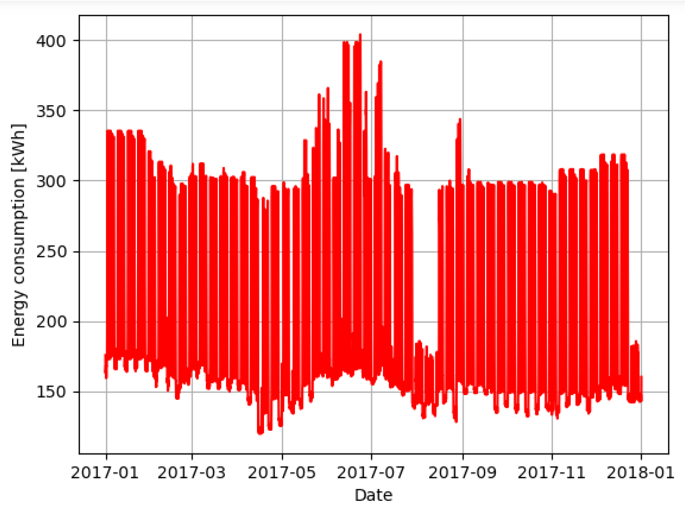
The synthetic data, free of data quality problems, are illustrated in Figure 3. This dataset was created to simulate the behavior of the GreEn-ER building, and it was based on its own electricity consumption.
From the data exposed in the previous figure, it is possible to notice different consumption patterns for different periods. It can be seen that the periods of higher consumption match with those of higher occupation, during daytime on the weekdays. Outside these periods, during nighttime on the weekdays, weekends, holidays and vacations, the consumption reduces drastically. In addition, it is possible to notice a relation with the temperature since the highest consumption occurs during summer.
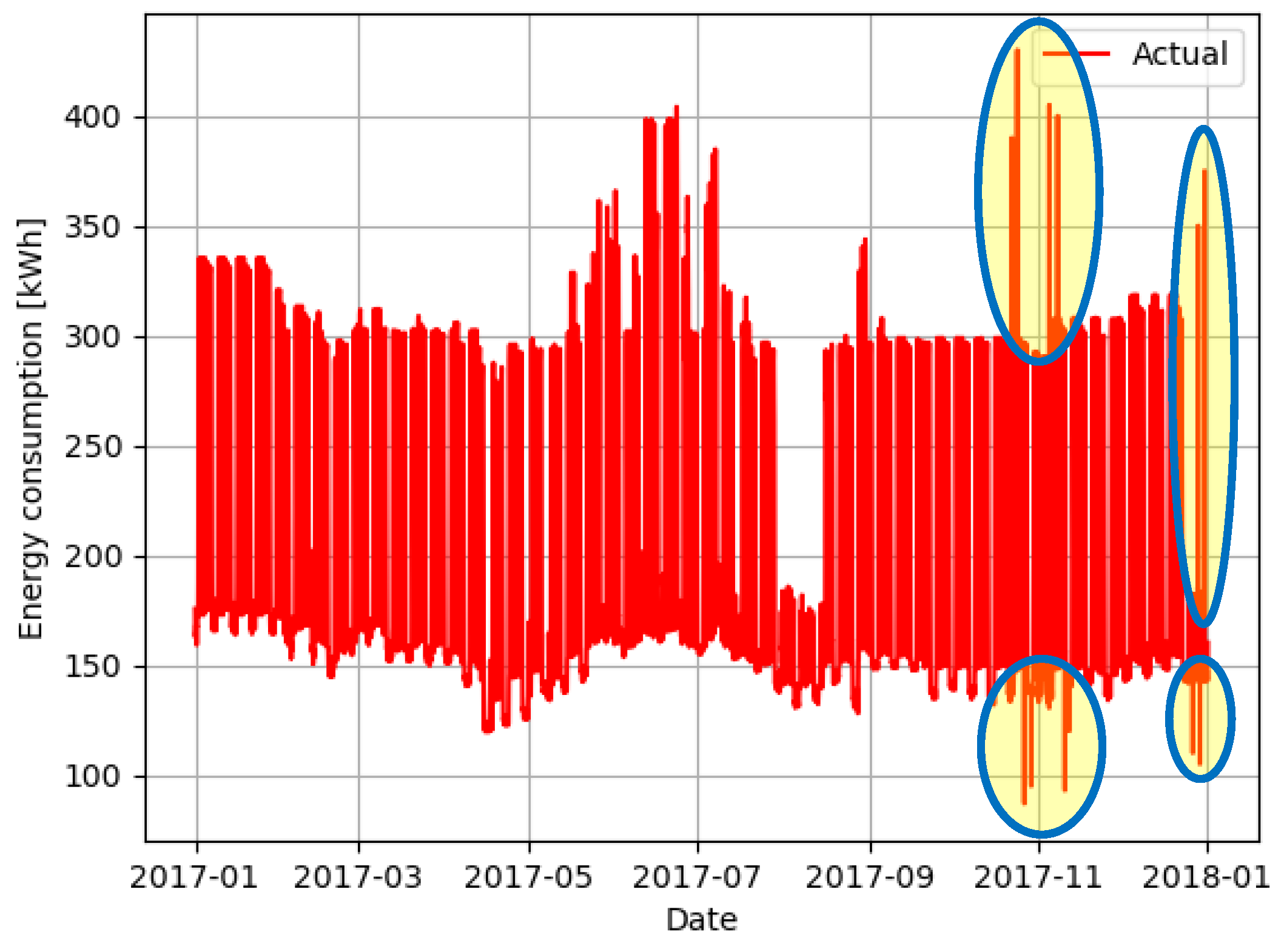
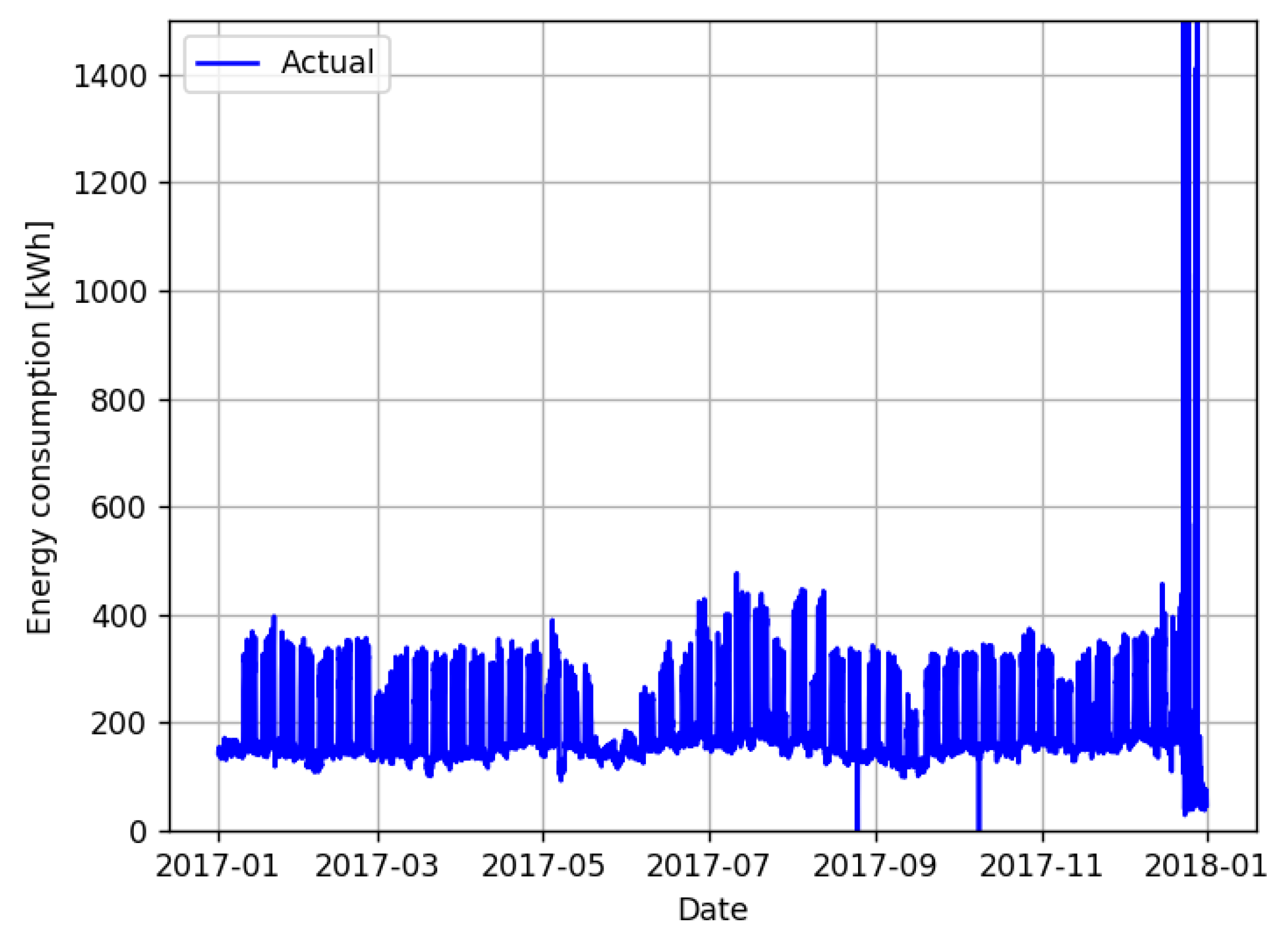
In order to test the outlier detection techniques, twelve outliers, both upper and lower, were manually introduced in the series presented in Figure 3, resulting in the dataset presented graphically in Figure 4. The information of these samples is shown in Table 1, and some of these outliers are highlighted in Figure 4 too. This information is then used as ground truth and compared with the results obtained to assess the classification of each sample in true positive, false positive and false negative.

4.1.1. Regression Methods Results

In order to find a model for the GreEn-ER energy consumption, the random forest method was applied using the data exposed in the previous section as the regression technique. For training of the algorithm, the following data features were used:
  • External temperature;
  • Average temperature of the day;
  • Time of the day;
  • Day of the year (with information of holidays and vacations).
The training dataset was defined as 80% of the data, from the beginning of the year until mid-October. All the outliers inserted in this dataset are concentrated beyond this period. These data quality problems make it difficult to assess the performance of the regressor only in test time interval because of their effect in the statistical variables (mean, median, standard deviation) used also to detect these abnormal samples. Because of that, the regressor performance was evaluated in two conditions. The first one considers the whole year, including the weeks with data quality problems and the training phase. The second one considers the period of the year complementary to the training phase. 
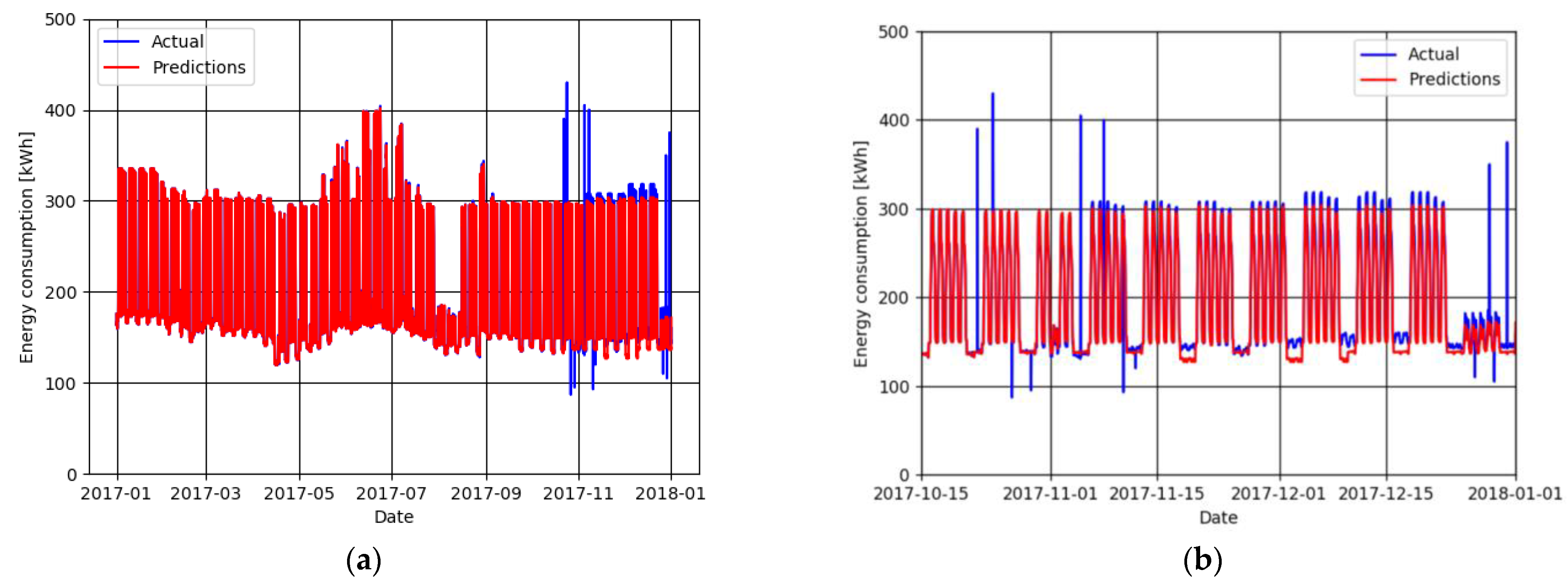
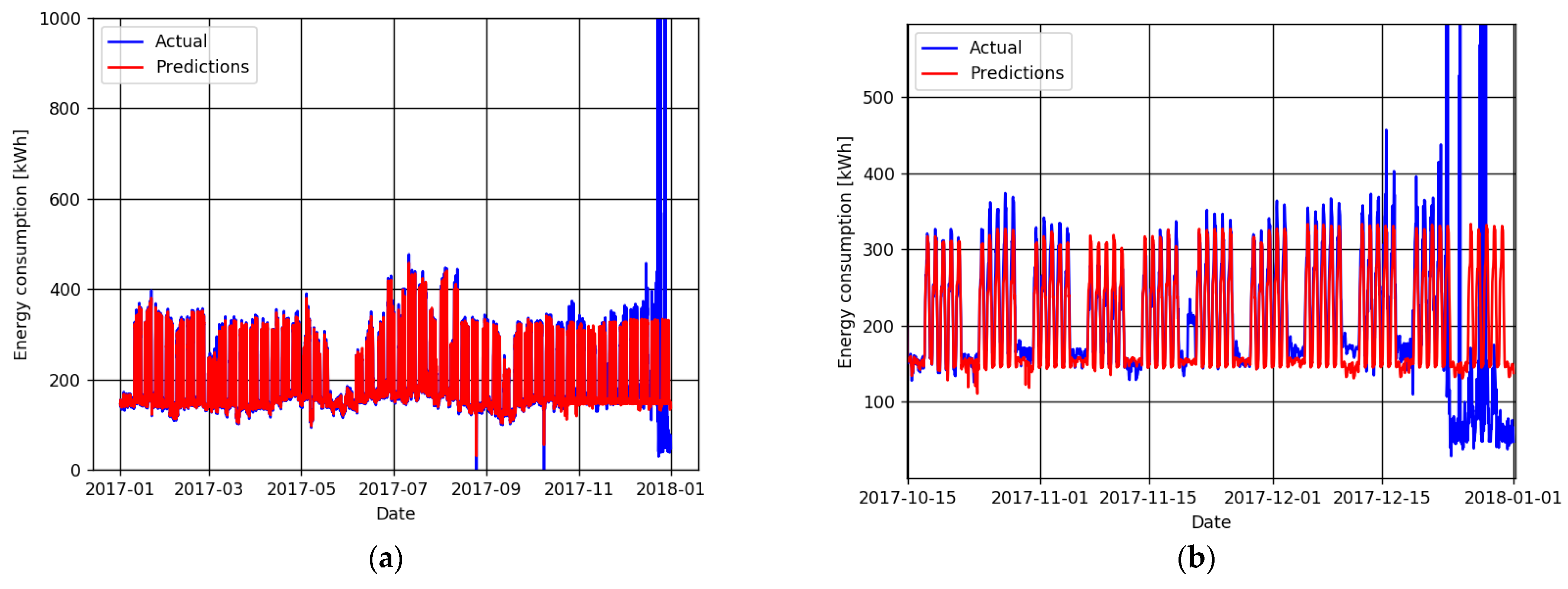
Figure 5 details, as an example, the results obtained with the application of the random forest method, using five hundred estimators as parameter. At the same time, Table 2 quantifies the performance of these regressions with the two conditions cited above.
Observing Figure 5b, only in the complementary period that was not used in the training phase are the results are satisfactory. Although the predictor underestimated the power on the weekends, it was able to detect the daily and weekly patterns and even during the holidays, resulting, on average, in less than a 5% error.
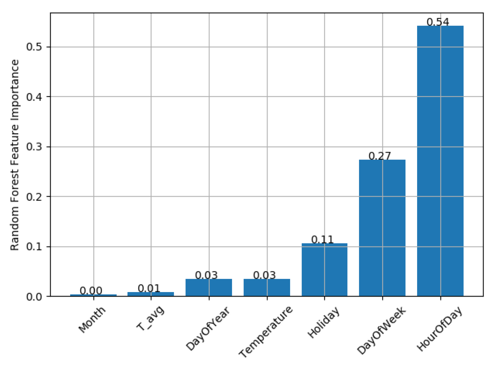
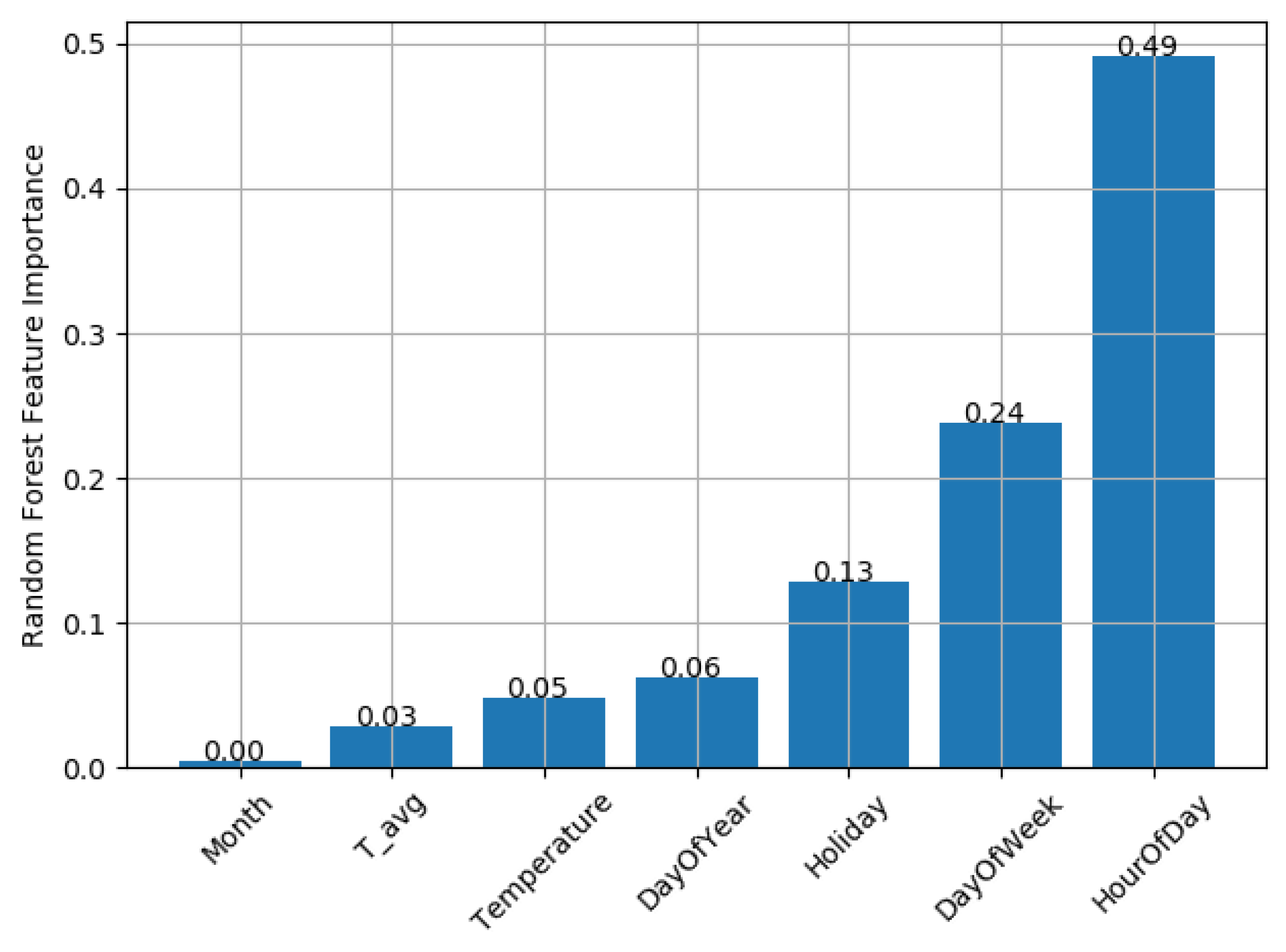
Regarding the regression, the most important features are the hour of the day, reproducing the daily pattern of the consumption, and the day of the week, reproducing the weekly shape of the load curve. The holiday feature also plays an important role in the performance of the regressor. The other features would be more important if more than a year’s worth of data were available. For instance, the external temperature would improve the regression inserting the season component, such as the difference between the days from summer and winter. However, with one year’s worth of data, and the choice of taking 80% of the series as training, this component is not important. These features were maintained in the model with the objective to improve the model in a future real time application, when more than a year would be available. Figure 6 shows the feature importance of the regression made for the adapted data.

4.1.2. Outlier Detection

In order to detect the outliers inserted in the data series, two strategies were applied. Primarily, a global search employing the statistical methods on the power consumption data was performed. Afterward, they were used to search outliers via the forecast error. Twelve outliers were manually inserted, six of them were upper outliers and the other six, lower, as shown in the previous section.
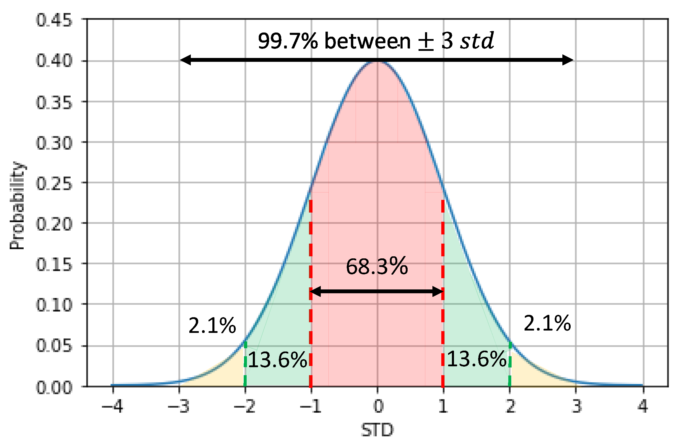
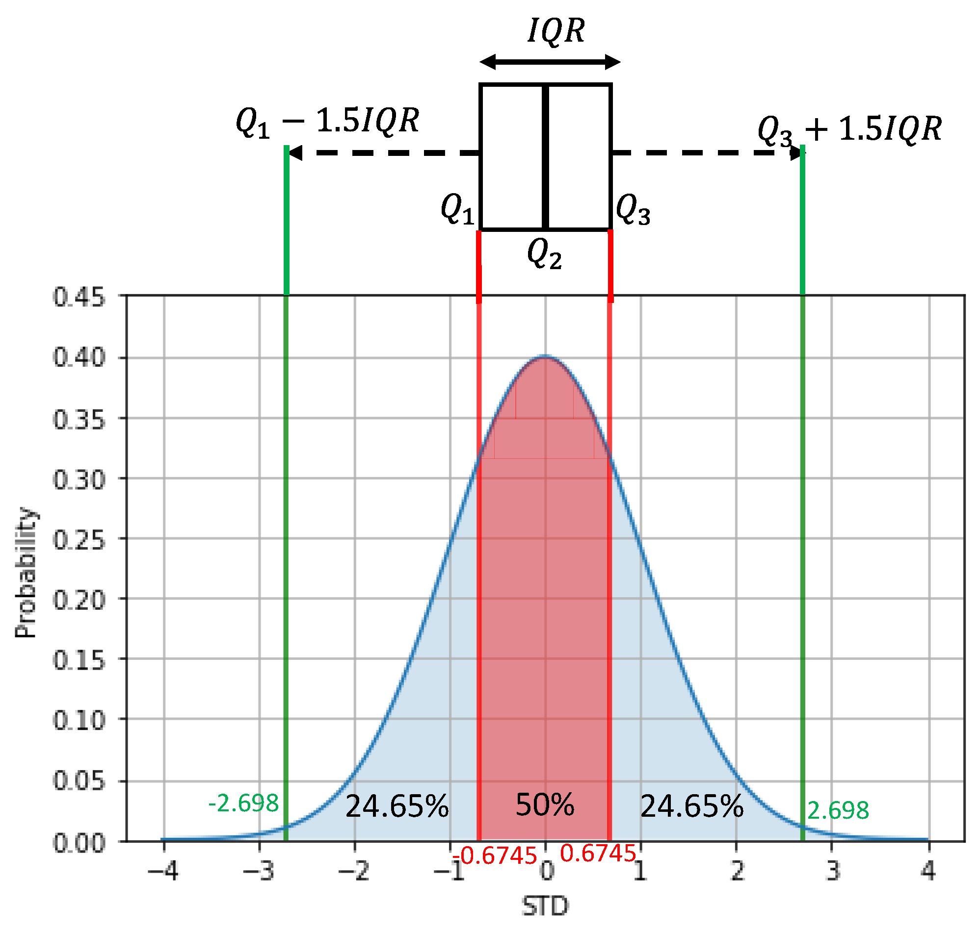
In the global search strategy, the search for outliers was performed only once. In this way, all information available is used, and the outliers are assumed to have any, or low, influence on the average value, the standard deviation, or even on the quartile values. Therefore, the global search was performed using the three-sigma rule, the boxplot, the skewed boxplot and the adjusted boxplot methods. The results are shown in Table 3. In this table, the column Potential Outliers Detected indicates the number of samples flagged out as outliers by each method. In the True Positives column, there are the number of actual outliers detected, while in the False Negatives column, the number of undetected outliers are presented. Furthermore, in the False Positives column, the number of normal samples misclassified as outliers are shown. Therefore, the sum of the true positives and the false negatives should be equal to the number of outliers present in the dataset, in this case, twelve. The sum of the true positives and false positives is equal to the potential outliers detected and the sum of both false positives and negatives gives the total of samples misclassified by each method.
The results indicate that the MAD and the adjusted boxplot were the most successful methods in detecting outliers, having found half of them; however, they still misclassified several other samples, reducing their precision. Thus, even detecting some outliers, their poor recall, with several false positive samples classified as outliers, show that these methods alone are not the best suitable to detect outliers, especially local ones, such as those inserted in this dataset.
As the classical statistical methods failed to detect several outliers in the study dataset, the forecast error method, which compares the results of previous regression models with measurements was employed. The statistical methods for outlier detection are then applied on the resulting error. Table 4 shows the number of outliers detected by each method considering the deviation between the actual values and the predictions.
The results presented in Table 4 indicate that the all the methods were able to detect most of the outliers inserted in the dataset, using the forecast error. However, the poor precision of the MAD, the boxplot, and the skewed boxplot misclassifying several samples indicates that they are not well suitable for this task in this dataset. The other two, three-sigma rule and adjusted boxplot, perform better and similarly, with a small advantage for the adjusted boxplot.

4.2. Real Data

The forecast error method was also tested in a dataset, available for downloading at the open science platform Mendeley Data [32], with no pre-treatment regarding data quality. This dataset was extracted directly from the GreEn-ER Building Management System and contains several problems of data quality, inherent to this type of monitoring. Figure 7 illustrates the power consumption data of the GreEn-ER building in which it is possible to visualize, for example, some outliers, values that extrapolate the scale of the graph, at the end of the year. In that period, both upper and lower outliers can be seen. A human agent looked through all samples and classified them into normal samples and upper (values higher than the normal instances) and lower (values lower than the normal instances) outliers, establishing the ground truth to which the results are compared to determine the true positives, false positives, and false negatives. Table 5 shows the type and the number of outliers found by the human agent.

4.2.1. Regression Methods Results

The procedure already shown in the previous section was also applied to the real data series. The random forest method was employed as the regression technique, with unmodified parameters and the results obtained are presented in Figure 8. The performance of the regression is quantified in Table 6.
Considering the complementary period, in Figure 8b, it can be seen that the predictor was able to reconstruct the daily and weekly patterns of the building consumption. The results are satisfactory, with less than 8% error on average, excluding the last week which contains numerous severe data quality problems. These anomalies are the ones that need to be pointed out, so the imperfection of the predictor is expected.
Regarding the importance of the features of the regression, similar results to the adapted data were obtained. Figure 9 shows the importance of each feature in the regression of the real data series.

4.2.2. Outlier Detection

As previously shown in Table 5, the outliers present in the series were manually classified to establish a benchmark for comparing the performance of the outlier detection algorithms. Two hundred and twelve outliers were found, eight of which are upper outliers and the other two hundred and four, lower.
The global search was performed using the three-sigma rule, the boxplot, the skewed boxplot and the adjusted boxplot methods. The results are shown in Table 7.
The presented results indicate that none of the tested methods were able to detect all the outliers. Furthermore, although the adjusted boxplot has initially pointed out more outliers than actually exist, it failed to detect forty outliers, and misclassified ninety-nine normal samples as abnormal data instances. Therefore, the results corroborate that those classical statistical methods applied to the value itself are not suitable to detect outliers, especially for local ones, such as the lower outliers present in this dataset.
As shown in the previous section, the forecast error method was also employed in the real data.
Although they found all outliers of the dataset, the results presented in Table 8 corroborate the notion that the MAD, the boxplot, and the skewed boxplot are not the most adapted methods to detect outliers using the forecast error in this dataset, as they misclassified several samples as outliers. Furthermore, the three-sigma rule failed to detect most of the outliers, flagging only the obvious upper outliers. Finally, the adjusted boxplot performed better, but still misclassified some samples. This method was able to detect 192 out of 212 outliers and misclassified another 13 samples as outliers, resulting in 33 misclassifications. This better performance of the adjusted boxplot can be seen by observing the F-score. While the MAD, the boxplot, and the skewed boxplot all have 1 recall, meaning that they found all the outliers (zero false negatives), their misclassification is costly as shown in their poor precision. This affects the F-score, decreasing its value. On the other hand, the adjusted boxplot presented the best compromise between the precision and the recall, resulting in both metrics to be higher than 0.90.

5. Conclusions

This work aimed to employ a hybrid method, called forecast error, to detect outliers in the power consumption of a tertiary building. This method combines regression methods with statistical outlier detection techniques. The random forest algorithm was used as the regression method and the three-sigma rule, the median absolute deviation, the boxplot, the skewed boxplot, and the adjusted boxplot were chosen as outlier detection techniques. In a global search, using only the statistical methods to the data instances themselves, none of them presented the expected performance. On the other hand, when the adjusted boxplot was applied to the forecast error (difference between the actual measurement and the forecast) better performance was obtained. Considering both datasets tested, this combination has presented the best F-score (higher than 0.90 in the real data dataset), but it was not perfect. Hence, a human-in-the-loop approach [34] is still needed, with the forecast error outlier detection method pointing out potential outliers and a human agent validating them. Thus, the effort would be less costly with the application of the method presented in this work.
In addition, this approach relies on high quality predictions, which may be improved. One way to improve the forecasts is using more features in the training phase. The consumption of one week earlier, in the case of the datasets pattern presented in this paper, is a common feature used. However, in the present dataset, with several subsequent samples with data quality problems, the use of the past consumption could degrade the model. On the other hand, in a real-time application, this feature could be of great help in the definition of a good predictor and would significantly improve the outlier and anomaly detection.

Supplementary Materials

The following are available online at https://gricad-gitlab.univ-grenoble-alpes.fr/martgust/power-consumption-data-quality, accessed on 17 November 2021, the source code and notebooks linked to this article.

Author Contributions

Conceptualization, G.F.M.N., P.K.-P. and F.W.; methodology, G.F.M.N., P.K.-P. and F.W.; validation, G.F.M.N.; data curation, G.F.M.N.; writing—original draft preparation, G.F.M.N.; writing—review and editing, N.J.B., P.K.-P. and F.W; supervision, F.W., P.K.-P., N.J.B. and B.D.; project administration, F.W. and P.K.-P.; funding acquisition, F.W. All authors have read and agreed to the published version of the manuscript.

Funding

The Carnot Énergies du Futur Institute, under the projects ORCEE and interebat, the French Centre National de la Recherche Scientifique (CNRS), the Grenoble-INP, the Université Grenoble Alpes (UGA), and the Federal University of Santa Catarina (UFSC) funded this research. This work has also been partially supported by the ANR (Agence Nationale de la Recherche) project eco-SESA (https://ecosesa.univ-grenoble-alpes.fr/ (accessed on 17 November 2021)) ANR-15-IDEX-02.

Institutional Review Board Statement

Not applicable.

Informed Consent Statement

Not applicable.

Data Availability Statement

The data presented in this study are openly available in Mendeley Data at DOI: 10.17632/h8mmnthn5w.1, reference number [32]. A resumed dataset can also be found in Supplementary Materials at: https://gricad-gitlab.univ-grenoble-alpes.fr/martgust/power-consumption-data-quality (accessed on 17 November 2021).

Conflicts of Interest

The authors declare no conflict of interest.

References

  1. Réseau de Transport D’éléctricité, “Bilan Électrique 2018”. 2019. Available online: https://bilan-electrique-2020.rte-france.com/wp-content/uploads/2019/02/BE-PDF-2018v3.pdf (accessed on 17 November 2021).
  2. Zhou, X.; Yang, T.; Liang, L.; Zi, X.; Yan, J.; Pan, D. Anomaly detection method of daily energy consumption patterns for central air conditioning systems. J. Build. Eng. 2021, 38, 102179. [Google Scholar] [CrossRef]
  3. Gaur, M.; Makonin, S.; Bajic, I.V.; Majumdar, A. Performance Evaluation of Techniques for Identifying Abnormal Energy Consumption in Buildings. IEEE Access 2019, 7, 62721–62733. [Google Scholar] [CrossRef]
  4. Himeur, Y.; Ghanem, K.; Alsalemi, A.; Bensaali, F.; Amira, A. Artificial intelligence based anomaly detection of energy consumption in buildings: A review, current trends and new perspectives. Appl. Energy 2021, 287, 116601. [Google Scholar] [CrossRef]
  5. Lee, D.; Lai, C.; Liao, K.; Chang, J. Artificial intelligence assisted false alarm detection and diagnosis system development for reducing maintenance cost of chillers at the data centre. J. Build. Eng. 2021, 36, 102110. [Google Scholar] [CrossRef]
  6. Lehmann, R. 3σ-Rule for Outlier Detection from the Viewpoint of Geodetic Adjustment. J. Surv. Eng. 2013, 139, 157–165. [Google Scholar] [CrossRef] [Green Version]
  7. Tukey, J.W. Exploratory Data Analysis; Addison-Wesley Publishing Company: Boston, MA, USA, 1977; p. 988. ISBN 0201076160. [Google Scholar]
  8. Wang, H.; Bah, M.J.; Hammad, M. Progress in Outlier Detection Techniques: A Survey. IEEE Access 2019, 7, 107964–108000. [Google Scholar] [CrossRef]
  9. Zhang, J. Advancements of Outlier Detection: A Survey. ICST Trans. Scalable Inf. Syst. 2013, 13, 1–26. [Google Scholar] [CrossRef] [Green Version]
  10. Satman, M.H. A New Algorithm for Detecting Outliers in Linear Regression. Int. J. Stat. Probab. 2013, 2, 101–109. [Google Scholar] [CrossRef]
  11. Abraham, B.; Chuang, A. Outlier Detection and Time Series Modeling. Technometrics 1989, 31, 241–248. [Google Scholar] [CrossRef]
  12. Ho, T.K. Random decision forests. In Proceedings of the 3rd International Conference on Document Analysis and Recognition, Montreal, QC, Canada, 14–16 August 1995; Volume 1, pp. 278–282. [Google Scholar] [CrossRef]
  13. Hubert, M.; Vandervieren, E. An adjusted boxplot for skewed distributions. Comput. Stat. Data Anal. 2008, 52, 5186–5201. [Google Scholar] [CrossRef]
  14. Hawkins, D.M. Identification of Outliers; Monographs on Applied Probability and Statistics; Springer: Dordrecht, The Netherlands, 1980; 188p, ISBN 9789401539944. [Google Scholar] [CrossRef]
  15. Vandeput, N. Data Science for Supply Chain Forecast; Independently published: Chicago, IL, USA, 2018; ISBN 978-1730969430. [Google Scholar]
  16. Breunig, M.M.; Kriegel, H.-P.; Ng, T.R.; Sander, J. LOF: Identifying Density-based Local Outliers. In Proceedings of the 2000 ACM SIGMOD International Conference on Management of Data, SIGMOD, Dallas, TX, USA, 15–18 May 2000; pp. 93–104, ISBN 1-58113-217-4. [Google Scholar] [CrossRef]
  17. Leys, C.; Ley, C.; Klein, O.; Bernard, P.; Licata, L. Detecting outliers: Do not use standard deviation around the mean, use absolute deviation around the median. J. Exp. Soc. Psychol. 2013, 49, 764–766. [Google Scholar] [CrossRef] [Green Version]
  18. Kimber, A.C. Exploratory Data Analysis for Possibly Censored Data from Skewed Distributions. J. R. Stat. Soc. Ser. C 1990, 39, 21–30. [Google Scholar] [CrossRef]
  19. Straker, D. Measuring Spread. Available online: http://www.syque.com/quality_tools/toolbook/Variation/measuring_spread.htm (accessed on 17 November 2021).
  20. Huber, P.J. Robust Statistics, 1st ed.; Wiley Series in Probability and Statistics; Wiley-Interscience: Hoboken, NJ, USA, 1981. [Google Scholar]
  21. Wickham, H.; Stryjewski, L. 40 Years of Boxplots, Had.Co.Nz. 2012. Available online: https://vita.had.co.nz/papers/boxplots.html (accessed on 17 November 2021).
  22. Olano, X.; de Jalón, A.G.; Pérez, D.; Barberena, J.G.; López, J.; Gastón, M. Outcomes and features of the inspection of receiver tubes (ITR) system for improved O&M in parabolic trough plants. AIP Conf. Proc. 2018, 2033, 030011. [Google Scholar] [CrossRef]
  23. Brys, G.; Hubert, M.; Rousseeuw, P.J. A robustification of independent component analysis. J. Chemom. 2005, 19, 364–375. [Google Scholar] [CrossRef]
  24. Kent, A.; Berry, M.M.; Luehrs, F.U.; Perry, J.W. Machine literature searching VIII. Operational criteria for designing information retrieval systems. Am. Doc. 1955, 6, 93–101. [Google Scholar] [CrossRef]
  25. Van Rijsbergen, C.J. Information Retrieval, 2nd ed.; Butterworth-Heinemann: Waltham, MA, USA, 1979. [Google Scholar]
  26. Zhao, H.; Tang, Z. The review of demand side management and load forecasting in smart grid. In Proceedings of the 12th World Congress on Intelligent Control and Automation (WCICA), Guilin, China, 12–15 June 2016; pp. 625–629. [Google Scholar] [CrossRef]
  27. Breiman, L.; Friedman, J.; Stone, C.J.; Olshen, R.A. Classification and Regression Trees; Wadsworth and Brooks: Monterey, CA, USA, 1984. [Google Scholar]
  28. HARP. Harp Random Forests. Available online: https://dsc-spidal.github.io/harp/docs/examples/rf/ (accessed on 17 November 2021).
  29. Sammut, C.; Webb, G.I. Mean Absolute Error. In Encyclopedia of Machine Learning; Springer: Boston, MA, USA, 2011. [Google Scholar] [CrossRef]
  30. De Myttenaere, A.; Golden, B.; Le Grand, B.; Rossi, F. Mean Absolute Percentage Error for regression models. Neurocomputing 2016, 192, 38–48. [Google Scholar] [CrossRef] [Green Version]
  31. Martin Nascimento, G.F.; Delinchant, B.; Wurtz, F.; Kuo-Peng, P.; Jhoe Batistela, N. “Power Consumption Data Quality”. Available online: https://gricad-gitlab.univ-grenoble-alpes.fr/martgust/power-consumption-data-quality (accessed on 17 November 2021).
  32. Martin Nascimento, G.F.; Delinchant, B.; Wurtz, F.; Kuo-Peng, P.; Jhoe Batistela, N.; Laranjeira, T. GreEn-ER—Electricity Consumption Data of a Tertiary Building. Mendeley Data, V1. 2020. Available online: http://dx.doi.org/10.17632/h8mmnthn5w.1 (accessed on 17 November 2021).
  33. Delinchant, B.; Wurtz, F.; Ploix, S.; Schanen, J.; Marechal, Y. GreEn-ER living lab: A green building with energy aware occupants. In Proceedings of the 5th International Conference on Smart Cities and Green ICT Systems (SMARTGREENS), Rome, Italy, 23–25 April 2016; pp. 1–8. [Google Scholar]
  34. Wurtz, F.; Delinchant, B. “Smart buildings” integrated in “smart grids”: A key challenge for the energy transition by using physical models and optimization with a “human-in-the-loop” approach. Comptes Rendus Phys. 2017, 18, 428–444. [Google Scholar] [CrossRef]
Figure 1. Percentages in normal distribution between standard deviations. Based on Straker [19].
Energies 14 08325 g001
Figure 2. Example of a box-and-whisker plot for a normal distribution. Based on Olano et al. [22].
Energies 14 08325 g002
Figure 3. Synthetic GreEn-ER global power consumption.
Energies 14 08325 g003
Figure 4. Synthetic GreEn-ER global power consumption with inserted outliers.
Energies 14 08325 g004
Figure 5. Regression results using the random forest algorithm on adapted data: (a) regression results and actual data during the whole year and (b) regression results and actual data during the period complementary to the training phase.
Energies 14 08325 g005
Figure 6. Data features’ importance in the random forest regression for the adapted data series.
Energies 14 08325 g006
Figure 7. Real GreEn-ER global power consumption with inserted outliers.
Energies 14 08325 g007
Figure 8. Regression results using the random forest algorithm on real data. (a) Regression results and actual data during the whole year and (b) regression results and actual data during the period complementary to the training phase.
Energies 14 08325 g008
Figure 9. Data features importance in the random forest regression of the real data series.
Energies 14 08325 g009
Table 1. Outliers inserted in the data series.
Outlier IndexTimestampDay of the WeekHoliday or VacationValue [kWh]Type of Outlier
122 October 2017 09:00SundayNo390Upper
224 October 2017 10:00TuesdayNo430Upper
326 October 2017 22:00ThursdayNo87Lower
429 October 2017 10:00SundayNo95Lower
54 November 2017 22:00SaturdayNo405Upper
67 November 2017 23:00TuesdayNo400Upper
710 November 2017 13:00FridayNo93Lower
812 November 2017 03:00SundayNo120Lower
926 December 2017 16:00TuesdayYes110Lower
1028 December 2017 14:00ThursdayYes350Upper
1129 December 2017 05:00FridayYes105Lower
1230 December 2017 21:00SaturdayYes375Upper
Table 2. Performance of the regression methods on the adapted data.
Error MetricPeriod
CompleteComplementary Period
MAE1.988.36
MAPE1%4.27%
Table 3. Number of outliers found in the global search by each method on adapted data.
MethodPotential Outliers DetectedTrue PositivesFalse NegativesFalse PositivesTotal MisclassificationsPrecisionRecallF-Score
3 Sigma11398170.2730.250.261
MAD808668028080.0070.50.015
Boxplot0012012000
Skewed Boxplot111101110.0830.154
Adjusted Boxplot826676820.0730.50.128
Table 4. Number of outliers found by the Forecast Error method applied to the random forest forecasts on the adapted data.
MethodPotential Outliers DetectedTrue PositivesFalse NegativesFalse PositivesTotal MisclassificationsPrecisionRecallF-Score
3 Sigma2311112130.4780.9170.628
MAD2136120212421240.00510.011
Boxplot1214120120212020.0110.02
Skewed boxplot1301120128912890.00910.018
Adjusted boxplot201119100.550.9170.688
Table 5. Number of outliers on real data found manually.
Upper OutliersLower OutliersTotal Outliers
8204212
Table 6. Performance of the regression methods on the Real Data.
Error MetricPeriod
CompleteComplementary Period 1
MAE12.0819.63
MAPE6.82%8.95%
1 Excluding last week.
Table 7. Outliers found in the global search by each method on real data.
MethodPotential Outliers DetectedTrue PositivesFalse NegativesFalse PositivesTotal MisclassificationsPrecisionRecallF-Score
3 Sigma66206020610.0280.055
MAD9311120192011210.0120.0520.019
Boxplot66206020610.0280.055
Skewed boxplot152151611620.9930.7120.83
Adjusted boxplot27117240991390.6350.8110.712
Table 8. Number of outliers found by the forecast error method applied to the random forest forecasts on the real data.
MethodPotential Outliers DetectedTrue PositivesFalse NegativesFalse PositivesTotal MisclassificationsPrecisionRecallF-Score
3 Sigma66206020610.0280.055
MAD14582120124612460.14510.254
Boxplot86021206486480.24710.396
Skewed boxplot105621208448440.20110.334
Adjusted boxplot2051922013330.9370.9060.921
Publisher’s Note: MDPI stays neutral with regard to jurisdictional claims in published maps and institutional affiliations.

