Outage Estimation in Electric Power Distribution Systems Using a Neural Network Ensemble

Abstract

Outages in an overhead power distribution system are caused by multiple environmental factors, such as weather, trees, and animal activity. Since they form a major portion of the outages, the ability to accurately estimate these outages is a significant step towards enhancing the reliability of power distribution systems. Earlier research with statistical models, neural networks, and committee machines to estimate weather-related and animal-related outages has reported some success. In this paper, a deep neural network ensemble model for outage estimation is proposed. The entire input space is partitioned with a distinct neural network in the ensemble performing outage estimate in each partition. A novel algorithm is proposed to train the neural networks in the ensemble, while simultaneously partitioning the input space in a suitable manner. The proposed approach has been compared with the earlier approaches for outage estimation for four U.S. cities. The results suggest that the proposed method significantly improves the estimates of outages caused by wind and lightning in power distribution systems. A comparative analysis with a previously published model for animal-related outages further establishes the overall effectiveness of the deep neural network ensemble.

1. Introduction

The reliability of an electric power distribution system indicates its ability to deliver power to the customers without interruptions. Due to their exposure to various hazards, overhead feeders, which are commonly used in distribution systems, contribute to the majority of service interruptions to the customers. Environmental factors such as weather, trees, and animals can be extremely hazardous for overhead feeders [1]. High wind and lightning not only cause damage directly to overhead lines, but they also break trees, which in turn can cause damage to the nearby feeders. Squirrels cause outages by creating short circuits across the insulators on the overhead feeders. Although complete prevention is not possible, proper design and maintenance can help in reducing weather- and animal-related outages to acceptable levels. Utilities keep records of outages, and based on that determine system upgrades to address the areas of higher outages. Most of the measures used today are retroactive in nature, where preventive decisions are made entirely upon past experience. Forecasting failures proactively from weather patterns can help utilities deal with outages much more effectively. Additionally, the normalization of reliability indices to weather allows them to have a better justification for the outages [1].

Since weather-related and animal-related outages are highly random, predicting their occurrence is a challenging task. Some basic approaches to model the causal relationships for outage prediction are based on statistical regression [2,3,4]. Simple neural networks that have been proposed to predict weather-related outages [5] have shown better performance than statistical models. However, as outages follow a very non-uniform distribution, there is a paucity of high outage samples in the training data. As a result, these neural networks tend to underestimate the frequency of outages during extreme environmental conditions. Several other neural network and machine learning approaches have been proposed for the prediction and analysis of outages [6,7,8,9,10,11,12,13,14,15]. While these methods have improved the results and provided better understanding of outages caused by weather and animals, there is still a need for research on the subject for further improvement in model performance. Motivated by the success of prior neural network approaches for the prediction of outages, this paper proposes a novel deep neural network approach for predicting outages in distribution systems that are caused by environmental factors.

Neural networks are layered structures containing simple processing units called neurons which are connected to one another though a set of weights [16,17]. Training the network involves iteratively incrementing the weights using a variant of the stochastic gradient descent algorithm, until the desired performance is achieved. Neural networks have shown to be remarkably successful in a wide range of pattern recognition tasks [18]. Their effectiveness has been clearly demonstrated in a variety of power grid applications [19,20,21].

Unlike classical deep regression networks that incorporate hidden layers which are fully connected [16,17], the intermediate stages of the present model are divided into independent blocks. Each block is a smaller neural network, which is trained independently of, but in parallel with, the other blocks, using a variation of the well-known backpropagation algorithm. The output stage of the model contains a specialized neuron (e.g., softmax neuron) that is capable of dividing the entire input space into non-overlapping partitions, so that each sub-network can be fine-tuned for any one partition. In other words, the proposed deep network applies a ‘divide-and-conquer’ strategy for outage estimation.

The partitioning the input space is based on the rationale that similar environmental conditions lead to similar outage levels. A neural network that is trained with a subset of samples containing only similar environmental inputs would predict outages with greater accuracy under those environmental conditions. Thus, better overall outage prediction can be attained by using an ensemble of separately trained, smaller neural networks than from any single network.

Another ensemble model for outage prediction (AdaBoost+) was proposed recently [5]. It showed marked improvement over statistical regression as well as simple neural networks. While AdaBoost+ is topologically very similar to the proposed model, it does not rely on a divide-and-conquer strategy; consequently, it applies a very different training algorithm using supervised learning. In contrast to AdaBoost+, a hybrid training algorithm that combines supervised and unsupervised learning is proposed in this research.

The main objective of this research is to develop an estimation method to address weather-related outages. Accordingly, the simulation results reported in this paper primarily focus on outages caused by wind and lightning. In order to establish the overall efficacy of the new approach as a generic model for outage estimation, comparisons with AdaBoost+ for animal related outages have also been briefly presented. The specific contributions of this research are in the following directions: (i) A new deep neural network ensemble is proposed to estimate weather-related outages in distribution systems. This model consistently outperformed existing methods in all four datasets used and in terms of all four performance measures (described later). (ii) The proposed model is also shown to be more accurate than AdaBoost+ for animal-related outages, again in terms of all metrics and datasets. (iii) A novel algorithm that contains aspects of supervised as well as unsupervised learning is proposed. The results indicate the effectiveness of this approach to train deep neural network ensembles. (iv) A theoretical justification of the overall approach is provided using a probabilistic graphical model framework.

The contents of the remainder of this paper are as follows: Section 2 provides a detailed description of weather-related outages, while also briefly addressing those caused by animal activity. The algorithmic aspects of the deep neural network ensemble are discussed in Section 3, while more theoretical issues are addressed subsequently in Section 4. Section 5 describes key results obtained from computer simulations, and Section 6 concludes this study.

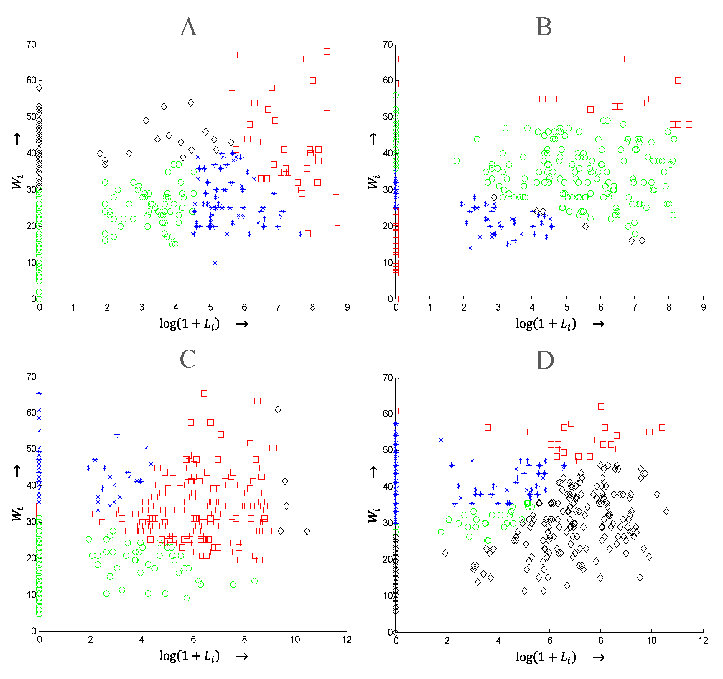
2. Outage and Weather Data

Outages due to weather and animals occur randomly and the probability of their occurrence increases during adverse conditions. For example, during stormy conditions due to high wind and lightning, the probability of outages increases. Similarly, the probability of outages due to animals increase under conditions that promote higher animal activity. Previous research showed that the aggregation of outages in space and time is necessary to obtain a meaningful a causal relationship [1,7,8]. The aggregation of outages over a day due to wind and lightning, and over a week due to animals, provide the best results.

An electric utility provided the recorded outage data for multiple years for the four cities considered for the research. Detailed weather information for these years was obtained from the local weather stations. The maximum daily 5-s wind gust speed measured in miles/hour was chosen to study wind effects because it has high correlation with the other measures of wind speeds. The absolute values of all the lightning strokes in kA, including the first stroke and the flashes in the defined area around the feeders, for each day of the study were added to find the aggregate of the lightning strokes for each of these days. Note that the earlier models [2,3,5] considered the lightning strokes recorded within 400 m of the distribution feeders. In contrast, the present study considers lightning strikes within 500 m. Furthermore, while only those days with lightning strikes were included earlier, in this approach, days without lightning are also included. The inputs to the model are the normalized wind and lightning data. The raw data from 2005 to 2009 was processed to identify outages caused by wind and lightning, and they were aggregated to create a database of daily outages.

Outages due to squirrels in the distribution systems of the same four cities in a period from 1998 to 2007 were considered to study animal-caused outages. The evaluation of squirrels’ yearly life cycle and animal-caused outage data showed that squirrels cause most damage in fair weather, which are the days with temperature within 40℉ and 85℉ with no other weather activity. Further, the behavioral patterns of squirrels are different in each month of the year, and thus months have considerable impacts on squirrel-related outages. Hence, the months were grouped into three groups based on the level of squirrel activity: Low (January, February, and March), Medium (April, July, August, and December), and High (May, June, September, October, and November). They are classified as Month Types 1, 2, and 3. The number of fair-weather days in each week were counted and they were classified into three levels, which are Low (zero fair weather days), Medium (one to three fair weather days), and High (four or more fair-weather days in the week). In addition, outages in the previous week due to animals were considered as an input to the model. They were classified into two categories (Low and High). The cutoff for High outage levels in the previous week is set at the 70th percentile, which means weeks with outages higher than those occurring in 70% of the weeks during the study are defined as High. The outages due to animals were aggregated to create a database of weekly outages.

3. Deep Neural Network Ensemble Approach

It is well-known that combining the outputs of an ensemble of neural networks (hereafter referred to as sub-networks) improves the overall performance [22]. In one such approach, the sensitivity of each sub-network to the output is used during training [23]. Another ensemble method decomposes the input space into Voronoi partitions (i.e., non-intersecting, convex partitions whose union is the input space) and associates a distinct sub-network for each partition. In [24], fuzzy C-means clustering is applied to partition the input space. In [25], a Boltzmann parameter has been used to reduce the degree of randomness of the genetic algorithm operators used in training. In another method [26], this parameter is steadily lowered but then reset to a high value to allow the neural networks to escape local minima.

In this research, the input space is indirectly partitioned by means of a softmax output neuron that also incorporates a Boltzmann parameter, which is initialized to a high value to allow the faster training of all sub-networks in the ensemble. As training progresses, it is steadily lowered so that the Voronoi partition boundaries become increasingly more pronounced. In the limiting case, when the Boltzmann parameter approaches zero, these boundaries are well-defined. This allows the output neuron to function as a switch, picking the output of the appropriate sub-network as the ensemble output. This arrangement also helps in avoiding overfitting [27].

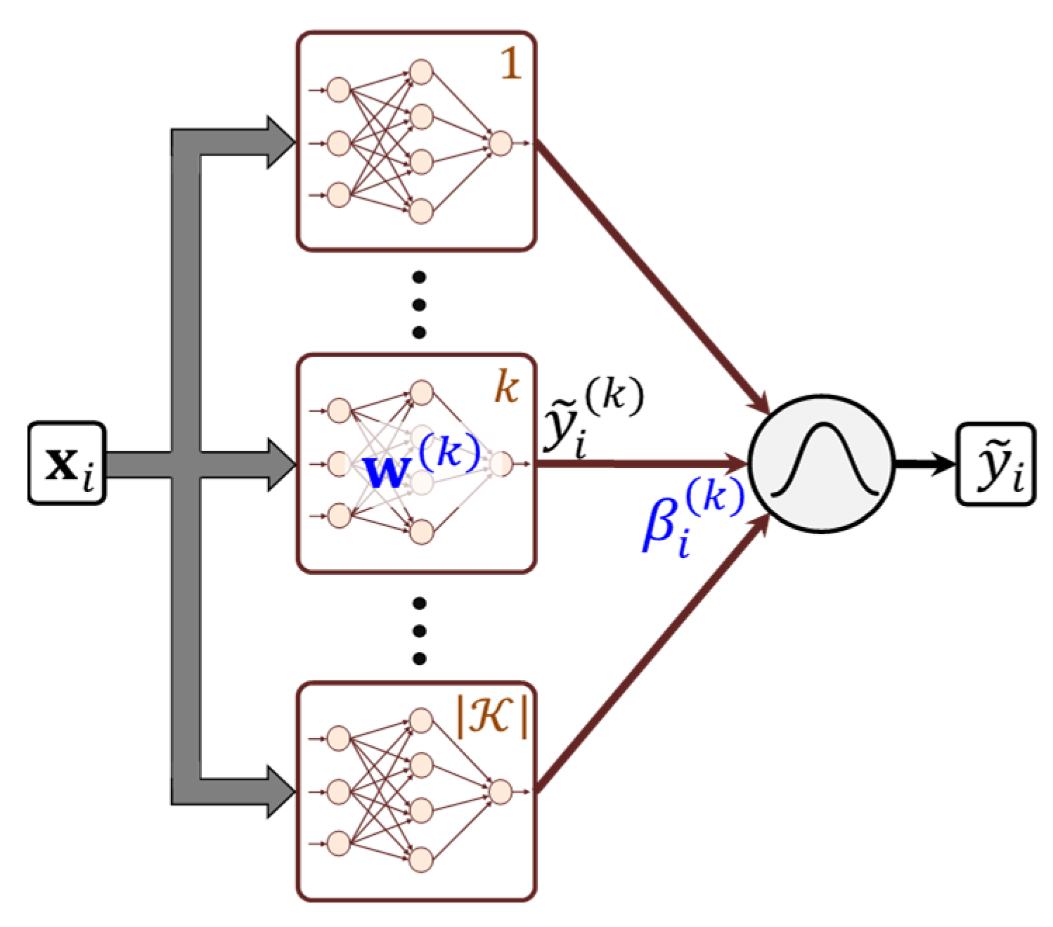
3.1. Layout of the Deep Neural Network Ensemble

The schematic in Figure 1 shows the layout of the deep neural network ensemble proposed in this research. The ensemble consists of a set of $\mathcal{K}$ sub-networks, where each is a $D\times H\times 1$ neural network, where $D$ and $H$ are the number of neurons in the input and hidden layers. Each hidden neuron realizes a sigmoidal saturating nonlinearity, while the output neuron is a weighted summing unit. The weights (including biases) of sub-network $k\in \mathcal{K}$ are collectively represented in terms of a vector, $w^{\left(k\right)}\in {ℝ}^{\left(D+2\right)H+1}$. A training sample consists of the input vector $x_i\in \mathcal{X}\subset {ℝ}_{+}^D$ and a scalar desired output, $y_i\in \left[0, y_{\max }\right]$, where $i\in \left\{1,\dots ,\left|\mathcal{N}\right|\right\}$, $\mathcal{N}$ is the training dataset, $\mathcal{X}$ is the input metric space, and $y_{\max }$ is the maximum possible failure experienced in the grid. The output of sub-network $k$ corresponding to the $i$th sample is denoted as ${\tilde{y}}_i^{\left(k\right)}$.

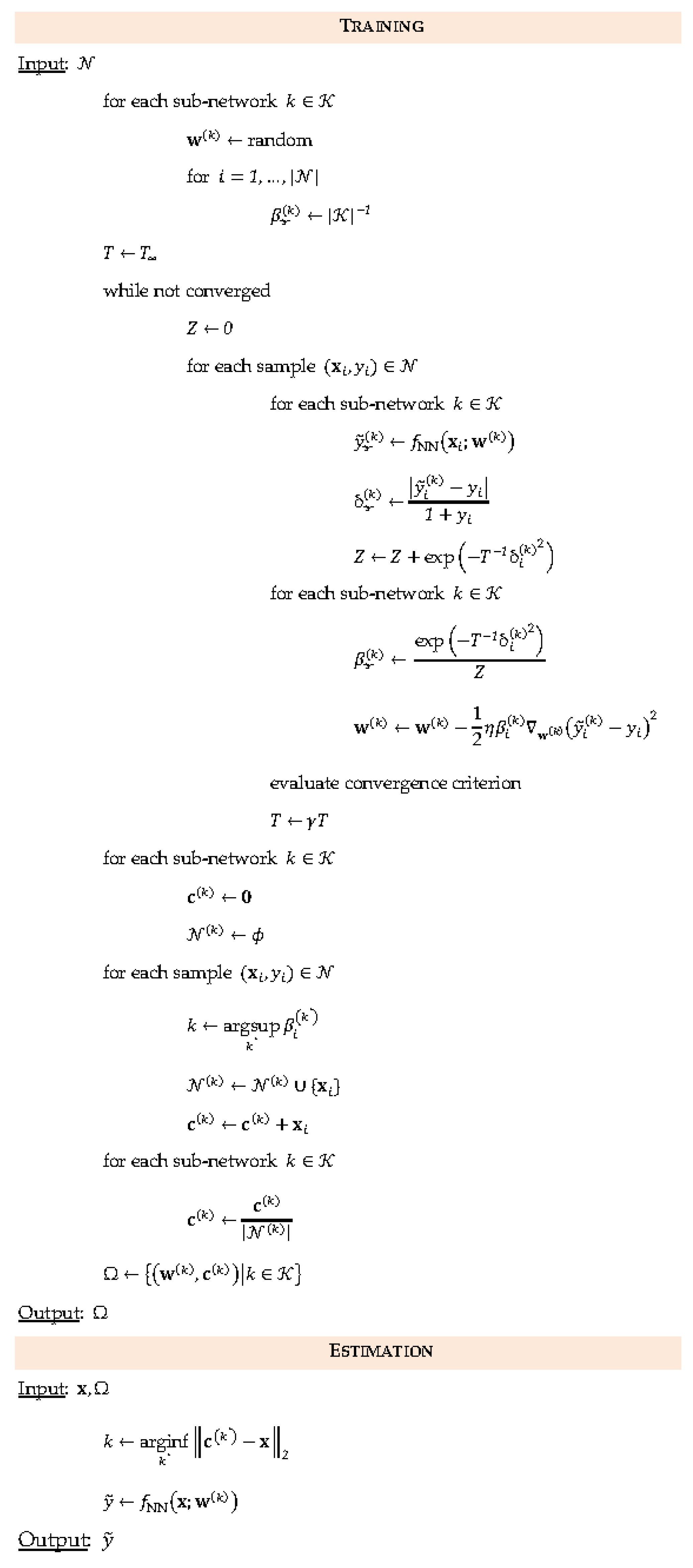
3.2. Supervised Learning in Sub-Networks

The sub-network $k$ is incrementally trained using weighted stochastic gradient descent as,

$$\begin{array}{c}{w}^{\left(k\right)}\leftarrow w^{\left(k\right)}-\frac{1}{2}\eta {\nabla }_{w^{\left(k\right)}}\left({\beta }_i^{\left(k\right)}{\left({\tilde{y}}_i^{\left(k\right)}-y_i\right)}^2+\xi R\left(w^{\left(k\right)}\right)\right)\end{array}$$

(1)

In the above expression, $\eta$ is the learning rate and the quantities ${\beta }_i^{\left(k\right)}\in \left(0,1\right)$ will be referred to as ensemble weights (Not to be confused with sub-network weights $w^{\left(k\right)}$). The optional second term is meant to regularize the weight vector with the ridge regression function $R(·)$; it can be excluded by setting the regularization parameter $\xi$ to zero. The weight updates in (1) can be algorithmically realized by means of a single step of backpropagation. The ensemble output is obtained as the weighted sum of the sub-network outputs,

$$\begin{array}{c}\underset{i}{\tilde{y}}={\displaystyle \sum _{k\in \mathcal{K}}}{\beta }_i^{\left(k\right)}{\tilde{y}}_i^{\left(k\right)}\end{array}$$

(2)

It is evident from the above expression that the quantity ${\beta }_i^{\left(k\right)}$ determines the weight assigned to sub-network $k$ in the ensemble output. Likewise, the update rule in (1) shows that the sub-network’s own weight vector $w^{\left(k\right)}$ is incremented in proportion to ${\beta }_i^{\left(k\right)}$. Each sub-network can be viewed as implementing some neural network function $f_{\mathrm{NN}}:\mathcal{X}\times {ℝ}^{\left(D+2\right)·H+1}\to \left[0, y_{\max }\right]$ so that,

$$\begin{array}{c}{\tilde{y}}_i^{\left(k\right)}\equiv f_{\mathrm{NN}}\left(x_i;w^{\left(k\right)}\right)\end{array}$$

(3)

This function $f_{\mathrm{NN}}(·)$ requires a forward pass through each sub-network. The expected absolute error over the entire dataset has an upper bound $\epsilon$ so that,

$$\begin{array}{c}E\left|{\displaystyle \sum _{k\in \mathcal{K}}}{\beta }_i^{\left(k\right)}{f}_{\mathrm{NN}}\left(x_i;w^{\left(k\right)}\right)-y_i\right|\le \epsilon \end{array}$$

(4)

The universal approximation theorem (cf. [28]) shows that as long as $\mathcal{K}$ is sufficiently large, then with proper training the upper bound $\epsilon$ can be made as small as possible, regardless of the probability distribution of the sample points in $\mathcal{X}$.

With $T$ denoting the Boltzmann parameter, the ensemble weights ${\beta }_i^{\left(k\right)}$ are determined according to the expression below:

$${\beta }_i^{\left(k\right)}=\frac{\exp \left(-T^{-1}{{\mathsf{\delta }}_i^{\left(k\right)}}^2\right)}{Z}$$

(5)

The denominator $Z$ in the above exponent is the partition function,

$$Z={\displaystyle \sum }_{k\in \mathcal{K}}\exp \left(-T^{-1}{{\mathsf{\delta }}_i^{\left(k\right)}}^2\right)$$

(6)

The purpose of the partition function is to normalize the ensemble weights so that ${\displaystyle \sum }_{k\in \mathcal{K}}{\beta }_i^{\left(k\right)}=1$. The quantity ${\mathsf{\delta }}_i^{\left(k\right)}$ is the normalized error. The error reflects the amount by which a sub-network estimate, ${\tilde{y}}_i^{\left(k\right)}$, deviates from the corresponding desired value, $y_i$. However, due to the wide range of the desired output values of $y_i$ (with $y_i=0$ being the most common, and higher values occurring increasingly infrequently), the absolute difference $\left|{\tilde{y}}_i^{\left(k\right)}-y_i\right|$ between the two quantities is normalized by dividing it with $1+y_i$, so that ${\mathsf{\delta }}_i^{\left(k\right)}$ can be interpreted as the fraction error. The 1 is included in the denominator to ensure that ${\mathsf{\delta }}_i^{\left(k\right)}$ stays finite when $y_i=0$ In accordance with these observations,

$${\mathsf{\delta }}_i^{\left(k\right)}=\frac{\left|{\tilde{y}}_i^{\left(k\right)}-y_i\right|}{1+y_i}$$

(7)

The expression in (5) shows that larger weights are assigned to sub-networks with lower ${\mathsf{\delta }}_i^{\left(k\right)}$, so that they are trained more with those samples for which they are more accurate. The role of the Boltzmann parameter $T$ is addressed in the next subsection.

3.3. Partitioning Using Unsupervised Learning

From (5) and (6), it can be seen that all sub-networks in the ensemble are weighted equally when $T$ is high,

$$\underset{T\to \infty }{\lim }{\beta }_i^{\left(k\right)}=\frac{1}{\left|\mathcal{K}\right|}$$

(8)

Accordingly, the Boltzmann parameter $T$ is initialized to a sufficiently high value, $T_{\infty }$, so that all training samples in the dataset $\mathcal{N}$ are equally utilized while training each sub-network. From another standpoint, $T=T_{\infty }$ corresponds to the situation where the input space is not decomposed into Voronoi partitions. Conversely, when $T\to 0$, ${\beta }_i^{\left(k\right)}$ is binary valued, being equal to unity only for the sub-network $k$ whose output ${\tilde{y}}_i^{\left(k\right)}$ is closest to its desired value $y_i$, and zero for all others. More specifically,

$$\underset{T\to 0}{\lim }{\beta }_i^{\left(k\right)}=\{\begin{array}{l}1, k=\underset{k^{\prime }}{\mathrm{arginf}}\left|{\tilde{y}}_i^{\left(k^{\prime }\right)}-y_i\right|\\ 0, otherwise\end{array}.$$

(9)

In this situation, the input space $\mathcal{X}$ is partitioned into a set of Voronoi regions ${\mathcal{X}}^{\left(k\right)}, k\in \mathcal{K}$, such that ${\mathcal{X}}^{\left(k\right)}\cap {\mathcal{X}}^{\left(k^{\prime }\right)}=\varphi$ whenever $k\ne k^{\prime }$, and ${{\displaystyle \cup }}_{k\in \mathcal{K}}{\mathcal{X}}^{\left(k\right)}=\mathcal{X}$. Suppose the input $x_i\in {\mathcal{X}}^{\left(k\right)}$ for some $k$, only the corresponding sub-network $k$ that yields the most accurate output is subjected to further training. The softmax output neuron functions as a switch, selecting the appropriate sub-network for input $x_i$, which is hereafter referred as the ‘winner’ sub-network. The intermediate values of $T$ have the effect of Voronoi partitioning $\mathcal{X}$ with ‘fuzzy’ boundaries as in [24]. At the end of each training epoch, the Boltzmann parameter is geometrically decreased by a factor $\gamma \in \left(0,1\right)$ (referred to as the ‘cooling’ rate) such that,

$$T\leftarrow \gamma T$$

(10)

The rate $\gamma$ is kept sufficiently close to unity to prevent the premature partitioning of $\mathcal{X}$.

Upon the termination of the gradient descent training procedure, each sample in $\mathcal{N}$ can be placed into its own Voronoi partitioned subset, ${\mathcal{N}}^{\left(k\right)}$,

$${\mathcal{N}}^{\left(k\right)}=\left\{x_i\in \mathcal{N}|k=\underset{k^{\prime }}{\mathrm{argsup}}{\beta }_i^{\left(k^{\prime }\right)}\right\}$$

(11)

The convexity of Voronoi partitions is well-established. Consequently, their centroids $c^{\left(k\right)}\in {\mathcal{X}}^{\left(k\right)}$ can be empirically estimated in the following manner,

$$c^{\left(k\right)}=\frac{1}{\left|{\mathcal{N}}^{\left(k\right)}\right|}{\displaystyle \sum }_{x_i\in {\mathcal{N}}^{\left(k\right)}}{x}_i$$

(12)

The weights and centroids are the sole parameters that fully define the ensemble $\mathsf{\Omega }$,

$$\mathsf{\Omega }\triangleq \left\{\left(w^{\left(k\right)}, c^{\left(k\right)}\right)|k\in \mathcal{K}\right\}$$

(13)

The other quantities, including ensemble weights, are no longer required after the ensemble has been fully trained. This is because the outage estimate $\tilde{y}$ of an unknown input $x\notin \mathcal{N}$ compares the distance from it to the centroids $c^{\left(k\right)}$ contained in $\mathsf{\Omega }$, and then uses the sub-network with the smallest distance, for the estimation. In other words,

$$\tilde{y}=f_{\mathrm{NN}}\left(x;w^{\left(k\right)}\right)$$

(14)

where $k$ is the winning sub-network, i.e.,

$$k=\underset{k^{\prime }\in \mathcal{K}}{\mathrm{arginf}}\Vert x-c^{\left(k^{\prime }\right)}{\Vert }_2$$

(15)

The steps involved in the training algorithm, as well as during estimating the outage for an unknown input $x$, are outlined in Figure 2. Initially, the sub-network weights $w^{\left(k\right)}$ are assigned small random values and $T$ is set to its maximum, $T_{\infty }$. Each iteration of the outer loop comprises of a training epoch, where all samples in the dataset $\mathcal{N}$ are sampled in a random order. In an epoch, each sub-network $k\in \mathcal{K}$ of the ensemble undergoes training in the following manner.

At first, the sub-network output ${\tilde{y}}_i^{\left(k\right)}$ is obtained through a forward pass (4). This is used to compute the normalized error ${\mathsf{\delta }}_i^{\left(k\right)}$, as in (7). To implement (6), the partition function is reset to 0 at the beginning of each epoch and is incremented in a stepwise manner. Next, the ensemble weights ${\beta }_i^{\left(k\right)}$ are computed as per (5), following which the sub-network weight $w^{\left(k\right)}$ is incremented as shown in (1). Note that the regularization term in (1) is not shown in Figure 2.

At the end of each epoch, $T$ is reduced as in (10). The convergence condition is satisfied either when the Boltzmann parameter $T$ acquires a very small value, or when the estimated averaged absolute error saturates at a steady value indicating that the stochastic gradient descent process has reached a minimum. Upon exiting the iterative process, the samples in $\mathcal{N}$ are placed in their own partitions, ${\mathcal{N}}^{\left(k\right)}$, as shown in (11). The last two steps of the training algorithm, involves computing the centroids $c^{\left(k\right)}$ and the ensemble $\mathsf{\Omega }$ in accordance with (12) and (13). The fully-trained ensemble can now be used to obtain a reliable estimate $\tilde{y}$ of the outages from an arbitrary input $x\notin \mathcal{N}$, as described in (14) and (15).

4. Theoretical Framework

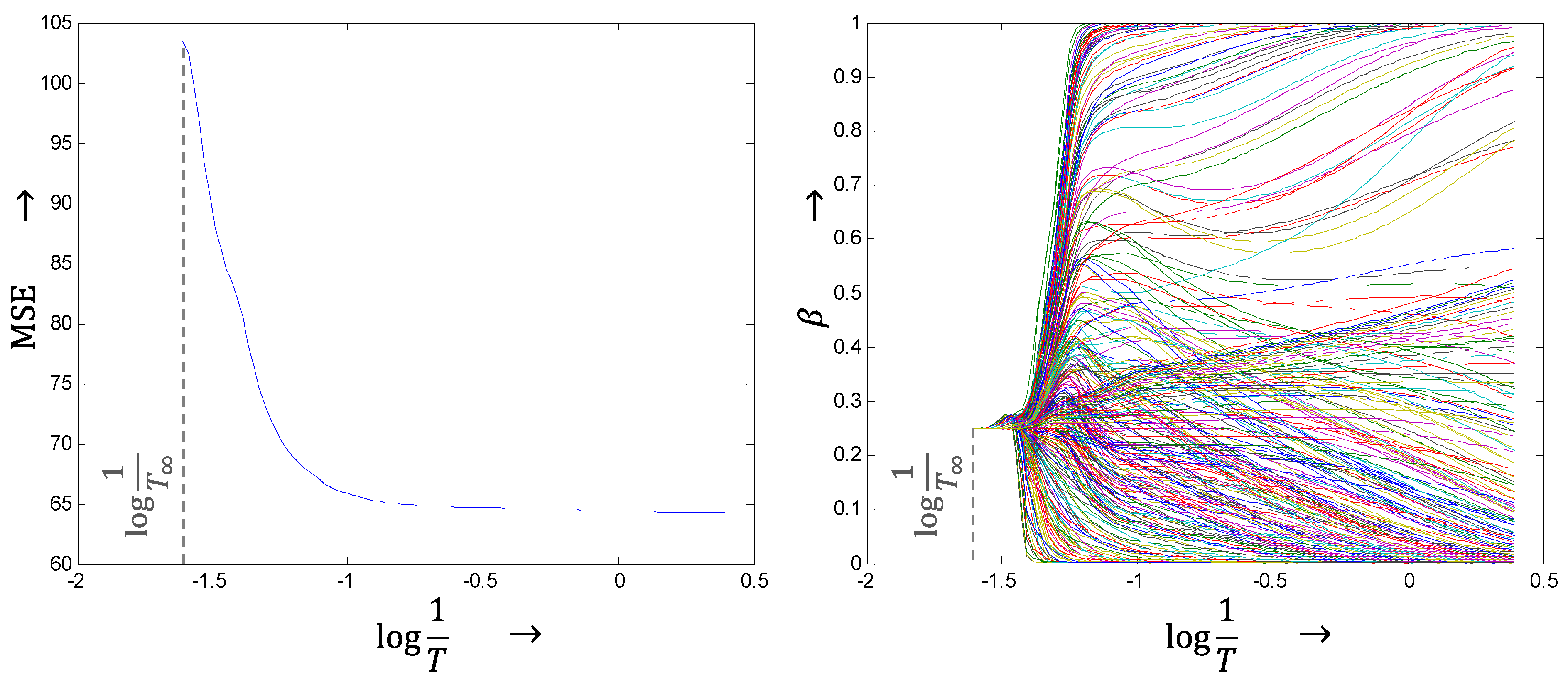
4.1. Gaussian Distribution Assumption

In this model, it is assumed that the probability of sub-network $k$ follows a Gaussian distribution with some constants $C$ and $\sigma$,

$$\mathrm{Pr}\left[f_{\mathrm{NN}}\left(x;w^{\left(k\right)}\right)=y\right]=C\exp \left(-\sigma \Vert x-{\mu }^{\left(k\right)}{\Vert }^2\right)$$

(16)

It can readily be shown that the maximum likelihood estimate $\tilde{y}$, given any input $x$, is obtained using the expressions provided earlier in (14) and (15). Let us define an assignment mapping $𝓀:\mathcal{X}\to \mathcal{K}$. For the sake of conciseness, given any sample $x_i\in \mathcal{N}$, let $𝓀\left(x_i\right)$ be written as ${𝓀}_i$. The joint probability of the dataset $\mathcal{N}$ is given by,

$$\mathrm{Pr}\left[\mathcal{N}\right]=C^{\left|\mathcal{N}\right|}{\displaystyle \prod }_{i\in \mathcal{N}}\exp \left(-\sigma \Vert x_i-{\mu }^{\left({𝓀}_i\right)}{\Vert }^2\right)$$

(17)

In order to maximize $\mathrm{Pr}\left[\mathcal{N}\right]$), the summation, ${{\displaystyle \sum }}_{i\in \mathcal{N}}\Vert x_i-{\mu }^{\left({𝓀}_i\right)}{\Vert }^2$, must be minimized. It follows that the optimal assignment ${𝓀}^{*}$ and Gaussian centers ${\mu }^{*\left(k\right)}$ are defined according to the expression below,

$$\left({𝓀}_i^{*},{\mu }^{*\left(k\right)}\right)=\underset{{𝓀}_i,{\mu }^{\left(k\right)}}{\mathrm{arginf}}{\displaystyle \sum }_{i\in \mathcal{N}}\Vert x_i-{\mu }^{\left({𝓀}_i\right)}{\Vert }^2$$

(18)

From (18), the optimal assignment can be determined in a straightforward matter since for each sample $x_i$,

$${𝓀}_i^{*}=\underset{k\in \mathcal{K}}{\mathrm{arginf}}\Vert x_i-{\mu }^{\left(k\right)}{\Vert }_2$$

(19)

It can be observed that (A4), shown above, is identical to the expression in (15), provided ${\mu }^{\left(k\right)}=c^{\left(k\right)}.$

Once the samples $x_i$ have been mapped to their respective partitions ${𝓀}_i^{*}$, we turn our attention to obtaining the optimal locations of the Gaussian means, ${\mu }^{*\left(k\right)}$. Let us define the partitions,

$${\mathcal{N}}^{\left(k\right)}=\left\{x_i|i\in \mathcal{N},k={𝓀}_i^{*}\right\}$$

so that the summation in (18) can be expressed as,

$${\displaystyle \sum }_{k\in \mathcal{K}}{\displaystyle \sum }_{i\in {\mathcal{N}}^{\left(k\right)}}\Vert x_i-{\mu }^{\left(k\right)}{\Vert }^2$$

It is evident that the inner summations ${\displaystyle \sum }_{i\in {\mathcal{N}}^{\left(k\right)}}\Vert x_i-{\mu }^{\left(k\right)}{\Vert }^2$ can be minimized separately for each $k$. It follows that,

$${\mu }^{*\left(k\right)}=\underset{{\mu }^{\left(k\right)}}{\mathrm{arginf}}{\displaystyle \sum }_{{\mathcal{N}}^{\left(k\right)}}\Vert x_i-{\mu }^{\left(k\right)}{\Vert }^2$$

(20)

It can be readily established using a few algebraic manipulations that the optimal Gaussian location is,

$${\mu }^{*\left(k\right)}=\frac{1}{\left|{\mathcal{N}}^{\left(k\right)}\right|}{\displaystyle \sum }_{x_i\in {\mathcal{N}}^{\left(k\right)}}{x}_i$$

(21)

The right-hand side of (21) is identical to that in (12), providing the rationale for selecting the winning sub-network in (15).

4.2. Markov Random Field Viewpoint

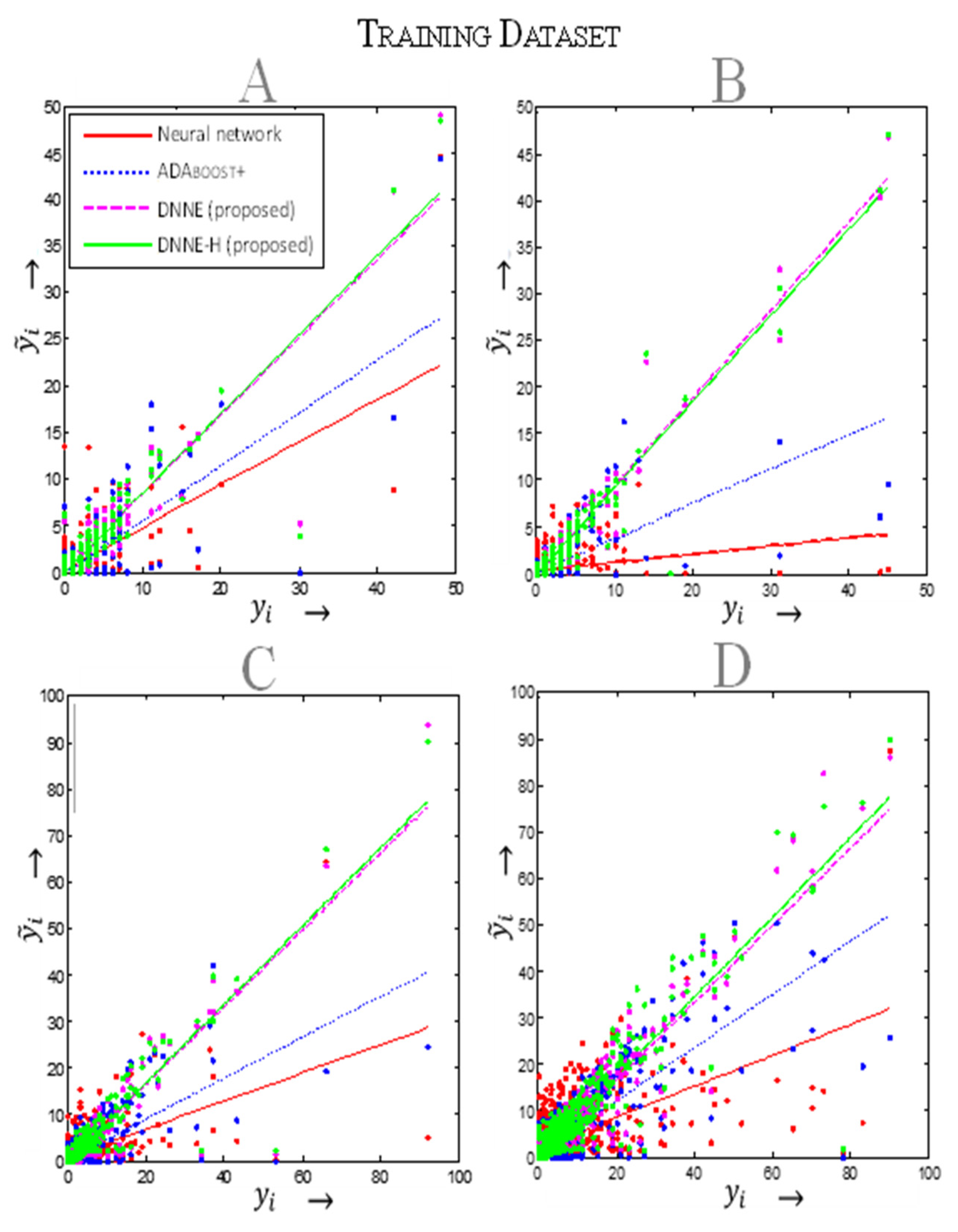
A Markov random field model interpretation [29] best illustrates the influence of the Boltzmann parameter $T$. Let each sample input $x_i\in \mathcal{N}$ in the dataset be treated as a vertex of a graph $\mathcal{G}\equiv \left(\mathcal{N},\mathcal{E}\right)$, where the set of edges is $\mathcal{E}\subset \mathcal{N}\times \mathcal{N}$. The graph $\mathcal{G}$ is undirected so that $\left(i,j\right)\in \mathcal{E}\iff \left(j,i\right)\in \mathcal{E}$. Furthermore, it is assumed that the vertices in $\mathcal{G}$ are divided into $\left|\mathcal{K}\right|$ maximal cliques, ${\mathcal{N}}^{\left(k\right)}, k\in \mathcal{K}$. All vertices in each ${\mathcal{N}}^{\left(k\right)}$ are assumed to be connected to one another so that $i,j\in {\mathcal{N}}^{\left(k\right)}\Rightarrow \left(i,j\right)\in \mathcal{E}$. A clique potential function $\mathsf{\Psi }:\mathcal{K}\to {ℝ}_{+}$ can be defined in the following manner,

$$\mathsf{\Psi }\left({\mathcal{N}}^{\left(k\right)}\right)\triangleq \frac{1}{2\left|{\mathcal{N}}^{\left(k\right)}\right|}{\displaystyle \sum }_{i,j\in {\mathcal{N}}^{\left(k\right)}}\Vert x_i-x_j{\Vert }_2^2$$

(22)

The energy of the system is the sum of all clique potentials,

$$H\left(\mathcal{N}\right)={\displaystyle \sum }_{k\in \mathcal{K}}\mathsf{\Psi }\left({\mathcal{N}}^{\left(k\right)}\right)$$

(23)

From the Hammersley-Clifford theorem [30], at any given value of $T,$ the joint probability of all outages in $\mathcal{N}$ is given by the Gibb’s distribution,

$$\mathrm{Pr}\left[\mathcal{N}\right]=\frac{\exp \left(-T^{-1}H\left(\mathcal{N}\right)\right)}{Z}$$

Using (22) and (23), the above probability is,

$$\mathrm{Pr}\left[\mathcal{N}\right]=\frac{1}{Z}\exp \left(-T^{-1}{\displaystyle \sum }_{k\in \mathcal{K}}\frac{1}{2\left|{\mathcal{N}}^{\left(k\right)}\right|}{\displaystyle \sum }_{i,j\in {\mathcal{N}}^{\left(k\right)}}\Vert x_i-x_j{\Vert }_2^2\right)$$

(24)

It is trivial to establish the following identity,

$${\displaystyle \sum }_{i,j\in {\mathcal{N}}^{\left(k\right)}}\Vert x_i-x_j{\Vert }_2^2=\frac{1}{2\left|{\mathcal{N}}^{\left(k\right)}\right|}{\displaystyle \sum }_{i\in {\mathcal{N}}^{\left(k\right)}}\Vert x_i-c^{\left(k\right)}{\Vert }_2^2$$

Using this identity, the joint probability in (24) reduces to,

$$\begin{array}{ll}\mathrm{Pr}\left[\mathcal{N}\right]& =\frac{1}{Z}\exp \left(-T^{-1}{\displaystyle {\displaystyle \sum }_{k\in \mathcal{K}}}{\displaystyle {\displaystyle \sum }_{i\in {\mathcal{N}}^{\left(k\right)}}}\Vert x_i-c^{\left(k\right)}{\Vert }_2^2\right)\\ & =\frac{1}{Z}{\displaystyle \prod _{i\in \mathcal{N}}}\exp \left(-T^{-1}\Vert x_i-c^{\left({𝓀}_i\right)}{\Vert }^2\right)\end{array}$$

(25)

It is evident that the expressions for the joint probability $\mathrm{Pr}\left[\mathcal{N}\right]$ in (25) and (16) are equivalent with the appropriate choice of centroids, with $\sigma =T^{-1}$. Steadily lowering the Boltzmann parameter $T$ as in (10) serves to increase this probability. This behavior is analogous to that observed in spin glass models in statistical physics.

5. Results

The four cities involved in this study are referred hitherto as A, B, C, and D, labeled according to their population sizes. Thus, city A is the least populous city, whereas city D is the largest. The available data were divided into training and test samples, separately for each city. In the following discussion, $\mathcal{N}$ could represent any of the four cities and either the training or the test dataset, depending on the context.

5.1. Performance Metrics

In order to analyze the performance of the proposed deep neural network ensemble (DNNE), the following metrics were used.

(i)

Mean Absolute Error:

$$\mathrm{MAE}=\frac{1}{\left|\mathcal{N}\right|}{\displaystyle \sum }_{i\in \mathcal{N}}\left|y_i-{\tilde{y}}_i\right|$$

(26)

It must be noted that since larger cities are expected to experience more outages, the MAE increases with city size, regardless of the model used.

(ii)

Mean Squared Error:

$$\mathrm{MSE}=\frac{1}{\left|\mathcal{N}\right|}{\displaystyle \sum }_{i\in \mathcal{N}}{\left(y_i-{\tilde{y}}_i\right)}^2$$

(27)

Due to the same reason as above, the MSE for city A will be the smallest, and that of city D, the highest.

(iii)

Slope: This is the slope of the best linear fit that passes through the origin.

$$\mathrm{S}=\underset{m\in \left(0,1\right]}{\mathrm{argmin}}{\displaystyle \sum }_{i\in \mathcal{N}}{\left({\tilde{y}}_i-m{y}_i\right)}^2$$

(28)

The larger values of $\mathrm{S}$ indicate better performance, with $\mathrm{S}=1$ being the limiting case of 100% accuracy.

(iv)

Coefficient of Correlation:

$$\mathrm{R}={\left({\displaystyle \sum }_{i\in \mathcal{N}}{\left({\tilde{y}}_i-{\tilde{\mu }}_y\right)}^2{\displaystyle \sum }_{j\in \mathcal{N}}{\left(y_j-{\mu }_y\right)}^2\right)}^{-\frac{1}{2}}{\displaystyle \sum }_{i\in \mathcal{N}}{\displaystyle \sum }_{j\in \mathcal{N}}\left({\tilde{y}}_i-{\tilde{\mu }}_y\right)\left(y_j-{\mu }_y\right)$$

(29)

where ${\tilde{\mu }}_y$ and ${\mu }_y$ are the average values of the estimated and actual outages. The larger values of $\mathrm{R}$ indicate better performance, with $\mathrm{R}=1$ being the limiting case of 100% accuracy.

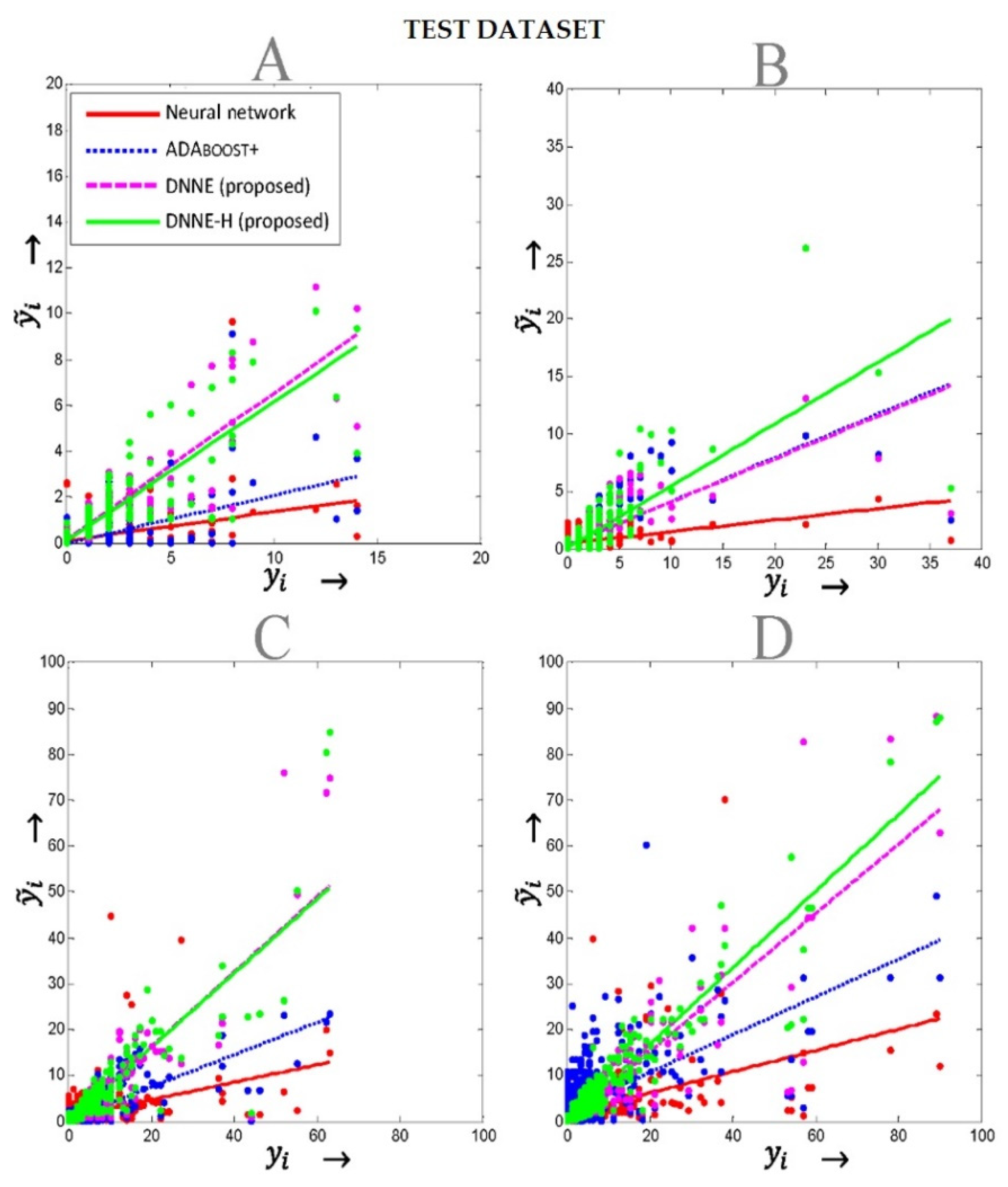
5.2. Weather-Related Outage Prediction

The daily outages due to wind and lightning, beginning in 2005 until the last day of 2011, were obtained from the utility company. The training dataset comprised of daily samples that were within the period 2005–2009, while the test dataset had daily samples from two years, 2010 and 2011. The values of the parameters were $\eta =0.2, \gamma =0.95,$and $T_{\infty }=5$. The weights $w^{\left(k\right)}$ were initialized to very small random initial values, and a maximum of 100 epochs was allowed, which was enough to ensure convergence while avoiding overfitting. As overfitting was not encountered, regularization was not used ($\xi =0)$.

Early experiments with first and second order polynomial regression strongly suggest that statistical methods may not be well-suited for outage estimation tasks. For conciseness, these results have not been reported in this section. Classical neural networks consistently outperformed them in all of the above metrics, corroborating earlier conclusions drawn with weather-related outages. Accordingly, neural networks and AdaBoost+ are the only two alternate methods adopted here for comparisons with the proposed DNNE. A cardinality $\left|\mathcal{K}\right|=4$ was found to be adequate for the purpose, with larger networks providing insignificant gains while increasing the computational burden.

Each sample (indexed $i$) contained the total daily lightning strikes $L_i$, daily maximum wind gust speed $W_i$, and the total outages $y_i$ due to wind and lightning for the day. Although the numerical range of $L_i$ for each city was very large, the distribution was highly skewed towards lower values. Hence, $\log \left(1+L_i\right)$ and $W_i$ were the two inputs to each model. This also allowed the inclusion of days with zero lightning in the analysis.

Initial investigations were carried out to draw insights into the convergence properties of the DNNE. Figure 3 shows the behavior of the learning algorithm as the Boltzmann parameter $T$, which is initialized to a high value of $T_{\infty }$, progressively decreases at the end of each training epoch. Figure 3 (left) shows how the MSE (scaled up by a factor $\left|\mathcal{K}\right|$) drops steadily with decreasing $T$. Figure 3 (right) shows the evolution of the quantities ${\beta }_i^{\left(k\right)}$. They are initialized to identical values of ${\left|\mathcal{K}\right|}^{-1}$ as in (8), so that the outputs of all sub-networks are weighted equally, as seen in (2). It can be observed that for each input $x_i$, the ${\beta }_i^{\left(k\right)}$ steadily increases for only a single sub-network $k$ in $\mathcal{K}$, while simultaneously decreasing for the remaining ones. Upon termination, when the MSE saturates to its asymptotic value, the values of ${\beta }_i^{\left(1\right)},\dots {\beta }_i^{\left(\left|\mathcal{K}\right|\right)}$ are differentiated enough to assign the samples to their eventual partitions. More interestingly, for a few initial training epochs, the ${\beta }_i^{\left(k\right)}$s do not show any perceptible differences. The onset of differences can be observed beyond a certain critical threshold ($\log T^{-1}\approx -1.4$). This observation is consistent with spin glass models in statistical physics where there exists a critical temperature below which particle spins within each domain align in the same directions. Although only the results of city D are shown in Figure 3, those of the other cities followed very similar patterns.

The final assignment of the samples to their respective partitions is shown in Figure 4, separately for all four cities. It can be observed that the distributions of real lighting strikes are heavily skewed towards $L_i=0$. Motivated by this observation, the task of weather-related outage estimation is extended so that one deep network is trained to handle samples with $L_i=0$, and the other, with $L_i>0$. This approach is abbreviated as DNNE-H (i.e., DNNE-Hybrid).

Table 1. Comparative performances of models for weather related outages.

City A (Weather)
Dataset	Training				Test
Metric	MAE	MSE	S	R	MAE	MSE	S	R
Neural Network	0.6009	2.4879	0.4555	0.6761	0.6433	2.3370	0.1254	0.4335
ADAboost+	0.3691	1.8251	0.5694	0.7860	0.5578	2.0558	0.2083	0.6079
DNNE	0.2611	0.7044	0.8406	0.9225	0.2802	0.6679	0.6400	0.8715
DNNE-H	0.2078	0.6390	0.8504	0.9294	0.2516	0.7266	0.6046	0.8674
City B (Weather)
Dataset	Training				Test
Metric	MAE	MSE	S	R	MAE	MSE	S	R
Neural Network	0.6973	4.3621	0.0871	0.2958	0.8778	5.0176	0.1012	0.4130
ADAboost+	0.3095	2.6210	0.3662	0.6947	0.4340	3.0395	0.3825	0.7173
DNNE	0.1815	0.2603	0.9414	0.9724	0.3856	2.9584	0.3743	0.7382
DNNE-H	0.1722	0.3762	0.9217	0.9610	0.4516	2.3559	0.5390	0.7867
City C (Weather)
Dataset	Training				Test
Metric	MAE	MSE	S	R	MAE	MSE	S	R
Neural Network	1.3913	12.9613	0.3016	0.5494	2.4418	37.1506	0.1909	0.4231
ADAboost+	0.7070	8.8922	0.4409	0.7448	1.4621	22.9910	0.3530	0.7928
DNNE	0.4493	3.0957	0.8276	0.9138	1.0227	9.6359	0.8172	0.8871
DNNE-H	0.4475	2.8011	0.8402	0.9217	0.9915	9.4382	0.8080	0.8882
City D (Weather)
Dataset	Training				Test
Metric	MAE	MSE	S	R	MAE	MSE	S	R
Neural Network	2.8051	35.9343	0.3312	0.5756	3.2873	76.7436	0.2314	0.4003
ADAboost+	1.4615	18.4254	0.5755	0.8263	2.4409	48.0201	0.3271	0.7963
DNNE	0.9677	8.1498	0.8289	0.9225	1.4358	18.6595	0.7524	0.8883
DNNE-H	0.0944	7.6422	0.8556	0.9262	1.1823	9.2845	0.8330	0.9473

shows the performances of the neural network, ADABoost+, DNNE, and DNNE-H. For each metric, the best performance is highlighted in bold. It can be clearly seen that in all cases, DNNE and DNNE-H outperformed the other models. Furthermore, in most cases, the performance of DNNE-H was marginally better than that of DNNE. Figure 5 and Figure 6 show the scatter plots of the observed and estimated outages obtained using all four models. The values of one for the regression coefficient (R) and the slope of the regression line (S) imply perfect prediction. The results illustrate the overall superior performance of the proposed approach in comparison to previous methods, with both R and S being closer to 1 in DNE and DNNE-H.

5.3. Animal-Related Outage Prediction

To investigate the effectiveness of DNNE for animal-related outage estimation, further simulations were carried out using animal related data, which involved the weekly outages of four cities, A, B, C, and D. Weekly outages during a nine year period between 1998 and 2006 were used as the training dataset; the test dataset comprised of outages that occurred in a single year, 2007. The sample inputs were $3\times 1$ vectors consisting of the number of fair-weather days of the week $F_i$, the month type $M_i$, and the outages $y_{i-1}$ of the immediately preceding week. The DNNE sub-networks were of size $3\times 5\times 1$ and the parameters were kept at $\eta =0.2, \gamma =0.95, \xi =0$, and $T_{\infty }=10$. The initial weights $w^{\left(k\right)}$ were very small random quantities. A cardinality $\left|\mathcal{K}\right|=4$ was used. A maximum of 150 epochs was allowed.

Table 2. Comparative performances of models for animal related outages.

City A (Animal)
Dataset	Training				Test
Metric	MAE	MSE	S	R	MAE	MSE	S	R
Neural Network	2.1843	9.8982	0.3021	0.5593	5.1144	1.8683	0.2867	0.3885
ADAboost+	0.8592	1.6513	0.8219	0.9518	0.6566	1.3111	0.5847	0.8325
DNNE	0.8246	1.5039	0.8576	0.9467	0.5576	0.9390	0.6624	0.8859
City B (Animal)
Dataset	Training				Test
Metric	MAE	MSE	S	R	MAE	MSE	S	R
Neural Network	3.1250	15.8521	0.4680	0.6857	3.7601	19.7885	0.4075	0.4263
ADAboost+	1.3293	3.5305	0.8170	0.9407	0.9759	2.4946	0.6102	0.8594
DNNE	1.2829	3.1367	0.8423	0.9468	0.9125	2.2260	0.6530	0.8739
City C (Animal)
Dataset	Training				Test
Metric	MAE	MSE	S	R	MAE	MSE	S	R
Neural Network	6.8084	84.4520	0.5896	0.7729	5.7810	54.3965	0.7059	0.7552
ADAboost+	2.8002	22.0193	0.8337	0.9485	2.6823	20.9659	0.7065	0.9589
DNNE	2.2725	11.0242	0.9344	0.9736	2.1174	11.4240	0.8028	0.9425
City D (Animal)
Dataset	Training				Test
Metric	MAE	MSE	S	R	MAE	MSE	S	R
Neural Network	8.6310	154.8318	0.5912	0.7800	6.2469	68.8767	0.9819	0.7399
ADAboost+	3.2699	33.8051	0.8637	0.9569	2.2847	12.5119	0.7104	0.9082
DNNE	2.8531	19.7962	0.9320	0.9741	1.8747	7.5639	0.8686	0.9333

shows the performances of a simple neural network, AdaBoost+, and the proposed DNNE in terms of the four metrics. It can be seen that the DNNE consistently outperformed the other models for the training datasets of cities B, C, and D. In city A, although AdaBoost+ yielded a value of $\mathrm{R}$ that is closer to unity than DNNE’s, the difference was too small (0.0051) to be of significance. The test data produced very similar patterns, with AdaBoost+ being marginally better in terms of $\mathrm{R}$ (0.0164) in city C. The only other anomalous pattern was in city D’s value of $\mathrm{S}$, where the neural network outperformed both AdaBoost+ and DNNE. This may be attributed to the large degree of randomness present in the datasets.

6. Conclusions

The objective of this paper is to propose a novel deep neural network approach for estimating weather-related outages in electric power distribution systems. The proposed method relies on a divide-and-conquer strategy to partition the entire input space into non-overlapping partitions, and a hybrid training algorithm that combines supervised and unsupervised learning is implemented, which under certain assumptions avoids overfitting. The results obtained for wind and lightning caused outages show that the accuracy of the proposed model shows a marked improvement over that of other models in predicting outages. In addition, the results indicate that separately estimating the outages of days with zero and nonzero lightning yielded further (albeit marginal) improvement in the prediction accuracy. Similarly, the results of animal-related outages with the proposed model show improvement over the previous models. While the proposed models show promising results, they still underestimate the outages caused by wind and lightning, and animals. More research is needed to further improve modeling for the estimation of these outages in power distribution systems.

The results presented in the paper are specific to the selected locations. Geographic features, climate, and other local factors can influence the results. However, the focus of the paper is to present a methodology, which can be applied at any location with some modifications.

7. Nomenclature

Frequently used symbols and their associated meaning are provided in

Table 3. Notation.

Symbol	Meaning
$\mathcal{K}$	Set of partitions (or sub-networks)
$D$	Dimensionality of input space
$H$	Number of hidden neurons in each sub-network
$\mathcal{X}$	Input space
$k$	Index of a partition or sub-network
${\mathcal{X}}^{\left(k\right)}$	Partition with index $k$
$w^{\left(k\right)}$	Vector of all weights (and biases) of sub-network $k$
$\mathcal{N}$	Dataset of samples (either training or test)
${\mathcal{N}}^{\left(k\right)}$	Subset of samples included in ${\mathcal{X}}^{\left(k\right)}$
$c^{\left(k\right)}$	Estimated centroid, i.e., mean of samples in ${\mathcal{N}}^{\left(k\right)}$
$i$	Index of a sample
$x_i$	$D\times 1$ input vector in any sample $i$
$y_i$	Real outage frequency in any sample $i$
${\tilde{y}}_i$	Estimated outage frequency in any sample $i$
${\tilde{y}}_i^{\left(k\right)}$	Output of sub-network $k$ for any sample $i$
$\eta$	Supervised learning rate
${\beta }_i^{\left(k\right)}$	Weight applied to any sample $i$ in sub-network $k$
$\xi$	(Optional) regularization parameter
$R(·)$	(Optional) regularization function
$f_{NN}(·)$	Sub-network output as a function of input and weights
$T$	Boltzmann parameter
$T_{\infty }$	Initial value of $T$
${\delta }_i^{\left(k\right)}$	Error in the output of sub-network $k$ for sample $i$(normalized)
$Z$	Partition function
$\gamma$	Cooling rate
$\Omega$	Set of all weights and centroids in the deep neural network ensemble
$MAE$	Mean absolute error
$MSE$	Mean squared error
$S$	Slope of regression line
$R$	Correlation coefficient
$L_i$	Total daily lightning strikes corresponding to sample $i$
$W_i$	Maximum daily wind gust speed corresponding to sample $i$
$F_i$	Level of fair-weather days in the week corresponding to sample $i$
$M_i$	Month type of the week corresponding to sample $i$
$y_{i-1}$	Level of outages in the previous week

below.

References

1. Caswell, H.; Forte, V.; Fraser, J.; Pahwa, A.; Short, T.; Thatcher, M.; Verner, V. Weather Normalization of Reliability Indices. IEEE Trans. Power Deliv. 2011, 26, 1273–1279. [Google Scholar] [CrossRef]
2. Kankanala, P.; Pahwa, A.; Das, S. Regression Models for Outages Due to Wind and Lightning on Overhead Distribution Feeders. In Proceedings of the IEEE PES General Meeting 2011, Detroit, MI, USA, 24–28 July 2011. [Google Scholar]
3. Kankanala, P.; Pahwa, A.; Das, S. Exponential Regression Models for Wind and Lightning Caused Outages on Overhead Distribution Feeders. In Proceedings of the North America Power Symposium (NAPS), Boston, MA, USA, 4–6 August 2011. [Google Scholar]
4. Doostan, M.; Chowdhury, B. Statistical Analysis of Animal-Related Outages in Power Distribution Systems–A Case Study. In Proceedings of the IEEE Power & Energy Society General Meeting (PESGM), Atlanta, GA, USA, 4–6 August 2019. [Google Scholar]
5. Kankanala, P.; Pahwa, A.; Das, S. Estimation of Overhead Distribution Outages Caused by Wind and Lightning Using an Artificial Neural Network. In Proceedings of the 9th International Conference on Power System Operation and Planning, Nairobi, Kenya, 16–19 January 2012. [Google Scholar]
6. Sahai, S.; Pahwa, A. A Probabilistic Approach for Animal–Caused Outages in Overhead Distribution Systems. In Proceedings of the Probability Methods Applications to Power Systems Conference, Stockholm, Sweden, 11–15 June 2006. [Google Scholar]
7. Gui, M.; Pahwa, A.; Das, S. Bayesian Network Model with Monte Carlo Simulations for Analysis of Animal-Related Outages in Overhead Distribution Systems. IEEE Trans. Power Syst. 2011, 26, 1618–1624. [Google Scholar] [CrossRef]
8. Kankanala, P.; Das, S.; Pahwa, A. AdaBoost+: An Ensemble Learning Approach for Estimating Weather-Related Outages in Distribution Systems. IEEE Trans. Power Syst. 2014, 29, 359–367. [Google Scholar] [CrossRef] [Green Version]
9. Kankanala, P.; Pahwa, A.; Das, S. Estimating Animal-Related Outages on Overhead Distribution Feeders using Boosting. In Proceedings of the 9th IFAC Symposium on Control of Power and Energy Systems, Delhi, New Delhi, 9–11 December 2015. [Google Scholar]
10. Sarwat, A.I.; Amini, M.; Domijan, A., Jr.; Damnjanovic, A.; Kaleem, F. Weather–based Interruption Prediction in the Smart Grid Utilizing Chronological Data. J. Mod. Power Syst. Clean Energy 2016, 4, 308–315. [Google Scholar] [CrossRef] [Green Version]
11. Pathan, A.; Timmerberg, J.; Mylvaganam, S. Some Case Studies of Power Outages with Possible Machine Learning Strategies for Their Predictions. In Proceedings of the 28th EAEEIE Annual Conference (EAEEIE), Hafnarfjordur, Iceland, 26–28 September 2018. [Google Scholar]
12. Tervo, R.; Karjalainen, J.; Jung, A. Predicting Electricity Outages Caused by Convective Storms. In Proceedings of the IEEE Data Science Workshop (DSW), Lausanne, Switzerland, 4–6 June 2018. [Google Scholar]
13. Nazmul Huda, A.S.; Živanović, R. An Efficient Method for Distribution System Reliability Evaluation Incorporating Weather Dependent Factors. In Proceedings of the 2019 IEEE International Conference on Industrial Technology (ICIT), Melbourne, Australia, 13–15 February 2019. [Google Scholar]
14. Sadegh Bashkari, M.; Sami, A.; Rastegar, M. Outage Cause Detection in Power Distribution Systems Based on Data Mining. IEEE Trans. Ind. Inform. 2021, 17, 640–649. [Google Scholar] [CrossRef]
15. Du, Y.; Liu, Y.; Wang, X.; Fang, J.; Sheng, G.; Jiang, X. Predicting Weather–Related Failure Risk in Distribution SystemsUsing Bayesian Neural Network. IEEE Trans. Smart Grid 2021, 12, 350–360. [Google Scholar] [CrossRef]
16. Sze, V.; Chen, Y.; Yang, T.; Emer, J.S. Efficient Processing of Deep Neural Networks: A Tutorial and Survey. Proc. IEEE 2017, 105, 2295–2329. [Google Scholar] [CrossRef] [Green Version]
17. Chiroma, H.; Abdullahi, U.A.; Abdulhamid, S.M.; Alarood, A.A.; Gabralla, L.A.; Rana, N.; Shuib, L.; Hashem, I.A.T.; Gbenga, D.E.; Abubakar, A.I.; et al. Progress on Artificial Neural Networks for Big Data Analytics: A Survey. IEEE Access 2019, 7, 70535–70551. [Google Scholar] [CrossRef]
18. Abiodun, O.I.; Jantan, A.; Omolara, A.E.; Dada, K.V.; Umar, A.M.; Linus, O.U.; Kazaure, A.A.; Gana, U.; Kiru, M.U. Comprehensive Review of Artificial Neural Network Applications to Pattern Recognition. IEEE Access 2019, 7, 158820–158846. [Google Scholar] [CrossRef]
19. Alimi, O.A.; Ouahada, K.; Abu-Mahfouz, A.M. A Review of Machine Learning Approaches to Power System Security and Stability. IEEE Access 2020, 8, 113512–113531. [Google Scholar] [CrossRef]
20. Quan, H.; Khosravi, A.; Yang, D.; Srinivasan, D. A Survey of Computational Intelligence Techniques for Wind Power Uncertainty Quantification in Smart Grids. IEEE Trans. Neural Netw. Learn. Syst. 2020, 31, 4582–4599. [Google Scholar] [CrossRef] [PubMed]
21. Massaoudi, M.; Abu-Rub, H.; Refaat, S.S.; Chihi, I.; Oueslati, F.S. Deep Learning in Smart Grid Technology: A Review of Recent Advancements and Future Prospects. IEEE Access 2021, 9, 54558–54578. [Google Scholar] [CrossRef]
22. Opitz, D.; Maclin, R. Popular ensemble methods: An empirical study. J. Artif. Intell. Res. 1999, 11, 169–198. [Google Scholar] [CrossRef]
23. Yang, J.; Zeng, X.; Zhong, S.; Wu, S. Effective Neural Network Ensemble Approach for Improving Generalization Performance. IEEE Trans. Neural Netw. Learn. Syst. 2013, 24, 878–887. [Google Scholar] [CrossRef] [PubMed]
24. Kim, E.; Oh, S.; Pedrycz, W.; Fu, Z. Reinforced Fuzzy Clustering-Based Ensemble Neural Networks. IEEE Trans. Fuzzy Syst. 2020, 28, 569–582. [Google Scholar] [CrossRef]
25. Soares, S.; Antunes, C.H.; Araújo, R. Comparison of a genetic algorithm and simulated annealing for automatic neural network ensemble development. Neurocomputing 2013, 121, 498–511. [Google Scholar] [CrossRef] [Green Version]
26. Dede, M.A.; Aptoula, E.; Genc, Y. Deep Network Ensembles for Aerial Scene Classification. IEEE Geosci. Remote. Sens. Lett. 2019, 16, 732–735. [Google Scholar] [CrossRef]
27. Perrone, M.P.; Cooper, L.N. When Networks Disagree: Ensemble Methods for Hybrid Neural Networks. In Neural Networks for Speech and Image Processing; Mammone, R.J., Ed.; Chapman-Hall: London, UK, 1993. [Google Scholar]
28. Musikawan, P.; Sunat, K.; Kongsorot, Y.; Horata, P.; Chiewchanwattana, S. Parallelized Metaheuristic-Ensemble of Heterogeneous Feedforward Neural Networks for Regression Problems. IEEE Access 2019, 7, 26909–26932. [Google Scholar] [CrossRef]
29. Freno, A.; Trentin, E. Markov Random Fields. In Hybrid. Random Fields: A Scalable Approach to Structure and Parameter Learning in Probabilistic Graphical Models (Intelligent Systems Reference Library); Springer: Berlin/Heidelberg, Germany, 2011; pp. 43–68. [Google Scholar]
30. Strauss, D.J. Hammersley-Clifford theorem. Encyclopedia of Statistical Sciences; Campbell, S.K., Read, B., Balakrishnan, N., Vidakovic, B., Johnson, N.L., Eds.; Wiley Interscience: Hoboken, NJ, USA, 2004; pp. 570–572. [Google Scholar]
Figure 1. Overall architecture of the proposed deep neural network ensemble (DNNE). Internal weights appear in blue fonts.
Energies 14 04797 g001
Figure 2. Outline of steps in the proposed approach.
Energies 14 04797 g002
Figure 3. Evolution of MSE (right) and β i ( k ) (left) with T for city D. Each trajectory (right) corresponds to a sample in dataset N , that appear in distinct colors for clarity.
Energies 14 04797 g003
Figure 4. Scatter plots of lightning L i vs. wind speed W i for each sample i in N , colored according to the Voronoi partition in K that contains i . Note that log ( 1 + L i ) has been used in the x-axis. Each plot corresponds to a city (AD).
Energies 14 04797 g004
Figure 5. Regression plots for training data. The points correspond the observed outages y i (x-axis) and estimated outages y ˜ i   (y-axis) for samples in the training dataset N using four different methods. The regression lines are also shown. A different color is used for each model (see legend on the top-left figure). Each plot corresponds to a city (AD).
Energies 14 04797 g005
Figure 6. Regression plots for test data. The points correspond to the observed outages y i (x-axis) and estimated outages y ˜ i   (y-axis) for samples in the test dataset N using four different methods. The regression lines are also shown. A different color is used for each model (see legend on the top-left figure). Each plot corresponds to a city (AD).
Energies 14 04797 g006