Article

An Adaptive Early Fault Detection Model of Induced Draft Fans Based on Multivariate State Estimation Technique

1
Inner Mongolia Power Research Institute, Hohhot 010020, China
2
School of Control and Computer Engineering, North China Electric Power University, Beijing 102206, China
3
Key Laboratory of Power Station Energy Transfer Conversion and System, North China Electric Power University, Beijing 102206, China
*
Author to whom correspondence should be addressed.
Energies 2021, 14(16), 4787; https://doi.org/10.3390/en14164787
Submission received: 4 July 2021 / Revised: 27 July 2021 / Accepted: 3 August 2021 / Published: 6 August 2021
(This article belongs to the Section K: State-of-the-Art Energy Related Technologies)

Abstract

:
The induced draft (ID) fan is an important piece of auxiliary equipment in coal-fired power plants. Early fault detection of the ID fan can provide predictive maintenance and reduce unscheduled shutdowns, thus improving the reliability of the power generation. In this study, an adaptive model was developed to achieve the early fault detection of ID fans. First, a non-parametric monitoring model was constructed to describe the normal operating characteristics with the multivariate state estimation technique (MSET). A similarity index representing operation status was defined according to the prediction deviations to produce warnings of early faults. To deal with the model accuracy degradation because of variant condition operation of the ID fan, an adaptive strategy was proposed by using the samples with a high data quality index (DQI) to manage the memory matrix and update the MSET model, thereby improving the fault detection results. The proposed method was applied to a 300 MW coal-fired power plant to achieve the early fault detection of an ID fan. In addition, fault detection by using the model without an update was also compared. Results show that the update strategy can greatly improve the MSET model accuracy when predicting normal operations of the ID fan; accordingly, the fault can be detected more than 4 h earlier by using the strategy with the adaptive update when compared to the model without an update.

1. Introduction

The induced draft (ID) fan is a mechanical device that exhausts the gas from other equipment with a wheel rotor to achieve gas compression and gas delivery. ID fans are widely used in ventilation plants, including mine, tunnel, and cooling towers. The ID fan is one of the crucial pieces of auxiliary equipment in the thermal power plant, where it induces the flue gas generated in the boiler to maintain a certain negative pressure in the furnace. ID fans are usually exposed to high-temperature flue gas and fly ash, which can make the impeller and blades easily eroded; moreover, the bearings are prone to wear and tear because of the mechanical vibration. Thus, faults can occur to ID fans in daily operations. Even worse, ID fan faults may cause an unscheduled downtime of the power plant, seriously affecting the secure operation and economic generation [1,2].
An early fault detection strategy can identify the current status based on historical operating information of process or equipment and give a warning signal on the abnormal operation, thereby providing enough time to take risk mitigation measures. Early fault detection models have been widely applied in different industrial fields [3,4,5,6,7]. Some models are developed according to the physical mechanism; however, it is usually difficult to obtain adequate knowledge for a non-linear complex industrial process, thus affecting the prediction accuracy in condition monitoring. Instead, researchers have tried to solve the fault detection problem by using historical operating data, also known as data-driven models. Shen et al. [8] employed an optimized deep belief network (DBN) technique to diagnose the bearing faults of the rotating machinery. Wang et al. [9] proposed an early fault detection for wind turbines based on operational condition clustering and optimized DBN. Francesc et al. [10] utilized principal component analysis to achieve wind turbine fault detection. Dai et al. [11] presented a fault detection strategy of the rolling bearing by combining sparse autoencoder (SAE) and denoising autoencoder (DAE).
In general, the abnormal operation can be identified by using classification techniques, including artificial neural networks (ANN), random forest, and support vector machines (SVM) [12,13,14,15,16,17,18]. Models are trained by using plenty of normal and abnormal operating data samples to produce accurate fault recognition results. For example, SVM is adopted in the classification of wind turbine faults with data sampled from supervisory control and data acquisition (SCADA) systems [17]. Guo et al. [18] introduced an improved random forest approach in fault recognition of direct current motors. These methods can divide the operating states into two types: fault states and fault-free states. To construct a precise model for fault detection, it is necessary to get the operating data of typical faults of the equipment or process. However, it is difficult to describe the dynamic characteristics of the ID fan with physical mechanism knowledge. The fault data samples of the ID fan are rarely recorded and not enough to train the model. In addition, it needs a large amount of computation to tune excessive adjustable parameters in the training process of machine learning models, and this is not conducive to field implementation in a power plant.
The multivariate state estimation technique (MSET) is one of the most used data-driven fault detection methods. The MSET model is developed with normal operating data, but unlike ANN, complicated parameter searching is not necessary during the MSET model construction, making it much easier and more feasible to be implemented in practical use [19,20,21,22,23,24,25,26,27]. By using MSET, faults can be detected without the need for fault records that are difficult to obtain, physical mechanism knowledge, and complicated parameter determination. MSET can learn the process features with historical normal operations and produce an estimation of the actual measured data sample, a process called the observation. By evaluating the similarity between the predicted value and the observation, operating faults can be identified. Thus, MSET can be used in constructing the early fault detection system of ID fans. MSET models have been wildly applied in the industrial field. For example, Zhang et al. [22] introduced the MSET model combined with similarity theory for early fault warning of auxiliary equipment; Cui et al. [23] integrated MSET with principal component analysis (PCA) to monitor the operating condition of an air compressor. Unlike model training of the ANN, the parameters of MSET can be directly solved by using the memory matrix.
MSET is a widely used data-driven method, and it mines the features of healthy states from the historical operating database. However, as with all the data-driven models, the accuracy of the MSET model has an important dependence on the training data, referred to a as a memory matrix, and represents the relationship among feature variables [27,28,29].
To obtain an accurate MSET model, the historic memory matrix usually consists of a set of operating data to represent all possible normal working conditions. Thus, how to construct an adequate memory matrix is crucial when applying MSET for early fault detection. As with preparing the training data of ANN models, the memory matrix needs to be elaborately designed, a process which has not received enough attention. In some research, several segments of data were manually selected from the plant-level operating database and then considered as the memory matrix. Such a method is implemented without any specific indicators; thus, all possible operating conditions cannot be fully covered. Another type of method tried to design the memory matrix with a uniform distribution by evenly selecting samples from historical operating data. Nevertheless, to the best of our knowledge, the memory matrix is usually set to be invariable in previous research. If the current operating conditions have a large change and deviate from the operating condition described by the memory matrix, the MSET model will exhibit a decline prediction accuracy, which is called model degradation. Model degradation is a crucial problem of the practical use of most data-driven models [30,31,32]. To maintain a high prediction accuracy, it is necessary to absorb operating information from newly acquired data and achieve the model update [33,34]. Model-update strategies have been presented to guarantee the prediction accuracy of the data-driven models. For example, Kaneko et al. [33] presented a review of adaptation mechanisms that are mainly utilized in data-driven modeling methods. In addition, Liu et al. [34] proposed kernel learning with adaptive parameter selection for soft sensor modeling of batch processes.
One commonly used framework for the adaptive update is the moving window strategy, in which the model is constructed with the most recent data of the window with a certain width that moves over time [35,36,37,38,39]. For example, Shi et al. [35] introduced a kernel function and the moving window algorithm to achieve real-time detection of rolling bearings faults; in Reference [36], the moving window was utilized to optimize the monitoring model based on the dynamic principal component analysis; and Sheriff et al. [37] proposed a moving window generalized likelihood ratio test approach to reduce the missed fault detection rate. The just-in-time (JIT) learning is another widely used update method. JIT learning method selects data samples that are similar to the observation from the historical operating database to construct the model; in addition, the model can be updated automatically by storing the newly acquired data into the database. Chen et al. [38] proposed a JIT-support vector regression model to achieve better silicon content prediction. Ahmad et al. [39] applied the JIT strategy to develop an online model. Both moving window and JIT learning strategies need to reconstruct the model with completely reselected data, and this process has an influence on the computation time and the sensitivity of the model.
To solve the above problems, the update of the MSET model can be implemented incrementally, in which the unnecessary sample is replaced and the update is executed once a new measured sample is acquired. The incremental update can reduce the computation cost compared with model reconstruction. In Reference [40], the incremental update was adopted to modify the parameters of the sequential assimilation model. Kaneko et al. [41] defined a database monitoring index to realize incremental updates and solve the model degradation problem. The index is used to measure information contained in newly acquired data and, thus, determine whether the new data are added to the database. Thus, the monitoring index can offer a valuable guide to designing the update strategy of the memory matrix, hence updating the MSET model.
The main contribution of this study is to introduce an adaptive early fault detection model for ID fans in coal-fired power plants. ID fan failure can cause the boiler to shut down unexpectedly, leading to power loss, high maintenance costs, and potential accidents. Early fault detection is an effective strategy to solve the above problems by producing a warning signal before the abnormality develops into a serious fault, allowing the operator time to take appropriate measures. The MSET method is utilized to detect early faults of ID fans in power plants in this study. The historic memory matrix used for the MSET model training consists of data samples that represent normal operating conditions. However, the operating conditions of the ID fan in power plants are inconstant because of the environmental change and boiler load regulation, and it is difficult to guarantee that all possible normal operating conditions are contained in the memory matrix when selecting training data from the plant-level database. If the ID fan runs beyond the coverage of the initially obtained memory matrix, an inaccurate estimation will be produced, thus leading to a false alarm. To solve the problem of variant condition operation of the ID fan and the model performance degradation, an adaptive update strategy is implemented to make the memory matrix cover newly acquired operating information. Based on the estimation errors of the MSET model, a similarity index is defined to detect potential faults of ID fans, thereby alarming the operators in advance.
The remainder of this paper is organized as follows. Section 2 describes the framework of the proposed adaptive MSET model, including the MSET theory, the adaptive update method, and the early warning approach. Section 3 presents a case study, and the results and discussion are also provided. Section 4 gives the conclusions.

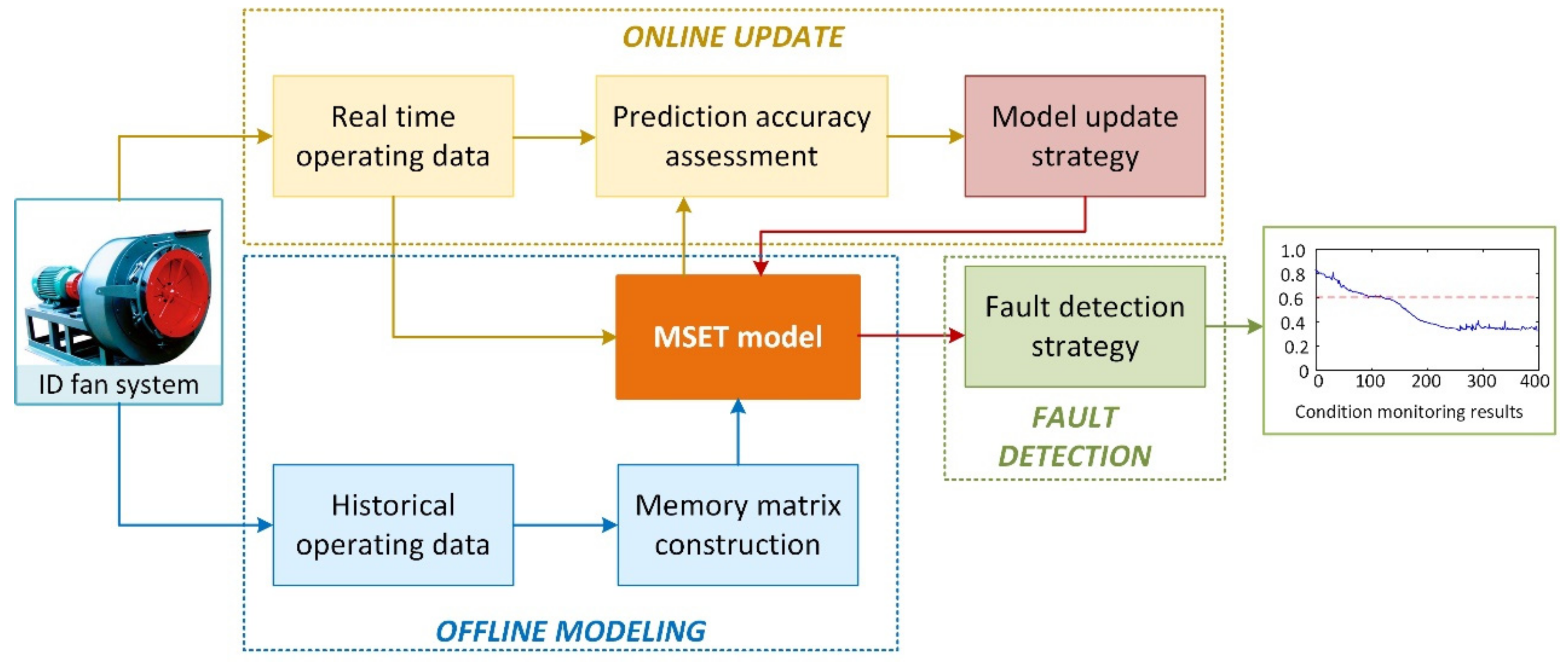
2. Adaptive Early Fault Detection Model Framework

2.1. Model Structure

The framework of the proposed adaptive early fault detection model is given in Figure 1. It consists of three parts: offline modeling, fault detection, and online update. The offline modeling module mainly develops the MSET model to calculate the estimation of the current observation; the online update module is used to achieve the update of the memory matrix and update the MSET model according to the prediction accuracy of the newly acquired operating data, and the fault detection module performs anomaly detection and produces warnings of early faults.
In the offline modeling module, the first step is to acquired historical normal operating data of the feature variables of the ID fan. One set of informative samples is selected from these data to construct the memory matrix and develop the MSET model. Then the real-time operating data are acquired and predicted by using the MSET model. The estimation deviations of the feature variables are taken as the inputs of the fault detection module to calculate the similarity index and achieve the condition monitoring of the ID fan system. If the similarity index is below the limit, a warning signal is produced to alert operators to take appropriate measures. In addition, the model prediction accuracy is assessed once a new measured data sample is obtained. According to the assessment results, the model update strategy is implemented if necessary to maintain a high prediction accuracy of the MSET model.

2.2. MSET Theory

MSET was first proposed by Argonne National Laboratory [19], and it is widely applied in condition monitoring, fault detection, and residual life prediction. The MSET model uses normal operating data, which are stored in the memory matrix, to characterize the monitored process or equipment. Considering that the memory matrix is constructed by a dataset of n variables at m time stamps, which are collected from the plant-level historical operating database, the memory matrix can be denoted as follows:
D   =   x t 1 , x t 2 , , x t m     =   x 1 t 1   x 1 t 2   x 2 t 1   x 2 t 2   x 1 t m   x 2 t m   x n t 1   x n t 2   x n t m  
where x i t j ( i = 1 ,   2 ,   ,   n , j = 1 ,   2 ,   ,   m , i and j are the indices of the variable and time stamp, respectively) is the value of the variable x i at time stamp t j . Each column of D represents a normal operation state at a certain time stamp, and each row represents the values of a certain variable at different time stamps. Thus, D consists of m vectors x t j that represent different normal operating states of a process.
For a given operating state, denoted as the observation vector, x o the MSET model will produce its estimation x ^ o by taking dot products between a weight vector, w , and the memory matrix, D :
x ^ o = D w = D     w 1 , w 2 , , w m T = w 1 x t 1   +   w 2 x t 2   +     +   w m x t m
As shown in Equation (2), the estimation vector, x ^ o , can be considered as a linear combination of m normal operating states with the weight vector ( w ). The estimation vector, x ^ o , is supposed to be like the observation vector, x o , if the equipment is in normal operations; that is, the residual ε between x ^ o and x o should be minimized. The residual ε can be written as follows:
ε = x o x ^ o
Then the quadratic sum of ε is written with respect to the weight vector, w :
J w   =   ε 2 = x o x ^ o T x o x ^ o = x o D w T x o D w   =   i = 1 n x o t i     j = 1 m w j D i j 2
where i = 1 ,   2 ,   ,   n , j = 1 ,   2 ,   ,   m , w k means the kth element of the weight vector w .
To get the minimum of the residual, we need to take the partial derivative of the J w to w k and make it equal to 0 :
J w w k = 2 i = 1 n x o t i     j = 1 m w j D i j D i k = 0
where i = 1 ,   2 ,   ,   n , j = 1 ,   2 ,   ,   m , k = 1 ,   2 ,   ,   m .
Namely,
i = 1 n x o t i D i k = i = 1 n j = 1 m w j D i j D i k = j = 1 m i = 1 n D i j D i k w j
where i = 1 ,   2 ,   ,   n , j = 1 ,   2 ,   ,   m , k = 1 ,   2 ,   ,   m .
Equation (6) can be written in a matrix form:
D T D w = D T x o
Then, the weight vector ( w ) can be calculated accordingly:
w = D T D 1 D T x o
As shown in Equation (8), the inversion of D T D is calculated to obtain the weight vector. The dot product calculation is replaced with a nonlinear operation, such as the Euclidean distance operation, to guarantee the existence of the inversion. The Euclidean distance φ is expressed as follows:
φ x , y   =   i = 1 n x i y i 2
Then Equation (9) can be expressed as follows:
w = K 1     f x o
where K is an m -by- m matrix, and K i j = φ D i , D j ; f is an m -by-1 function vector, and f i = φ D i ,   x o , D i = x t i . K i j is the i th row and j th column element of K .
Thus, the weight vector can represent the similarity of x o and D . Assuming that the observation vector ( x o ) is very similar to the vector x t i in D , the weight ( w i ) can have a large value. After submitting Equation (10) into Equation (2), the estimation vector ( x ^ o ) can be written as follows:
x ^ o = D K 1 f x o
If the observation, x o is consistent with most vectors in memory matrix ( D ), the estimation vector ( x ^ o ) will be close to x o . On the contrary, if a potential fault occurs, the observation ( x o ) will diverge from normal operating states, and an estimation vector with large deviations is generated.
The memory matrix ( D ) needs to be constructed firstly when developing the MSET model. The data samples in D should cover all possible operating conditions to characterize the ID fan system. However, the historical operating data recorded in the plant-level database is large in volume, and if the memory matrix ( D ) is constructed with all operating data, the computational complexity will increase greatly, leading to a decline in real-time warning performance. Thus, the memory matrix ( D ) should be selected according to a well-designed criterion. In this way, the samples in the memory matrix ( D ) can be representative to guarantee good prediction accuracy of the developed MSET model. There are many sample-selection methods, such as uniform sampling method, random sampling method, etc. In this paper, the memory matrix ( D ) is constructed by maximizing the operating information with optimization algorithms, which is detailed in Reference [42].

2.3. Fault Detection
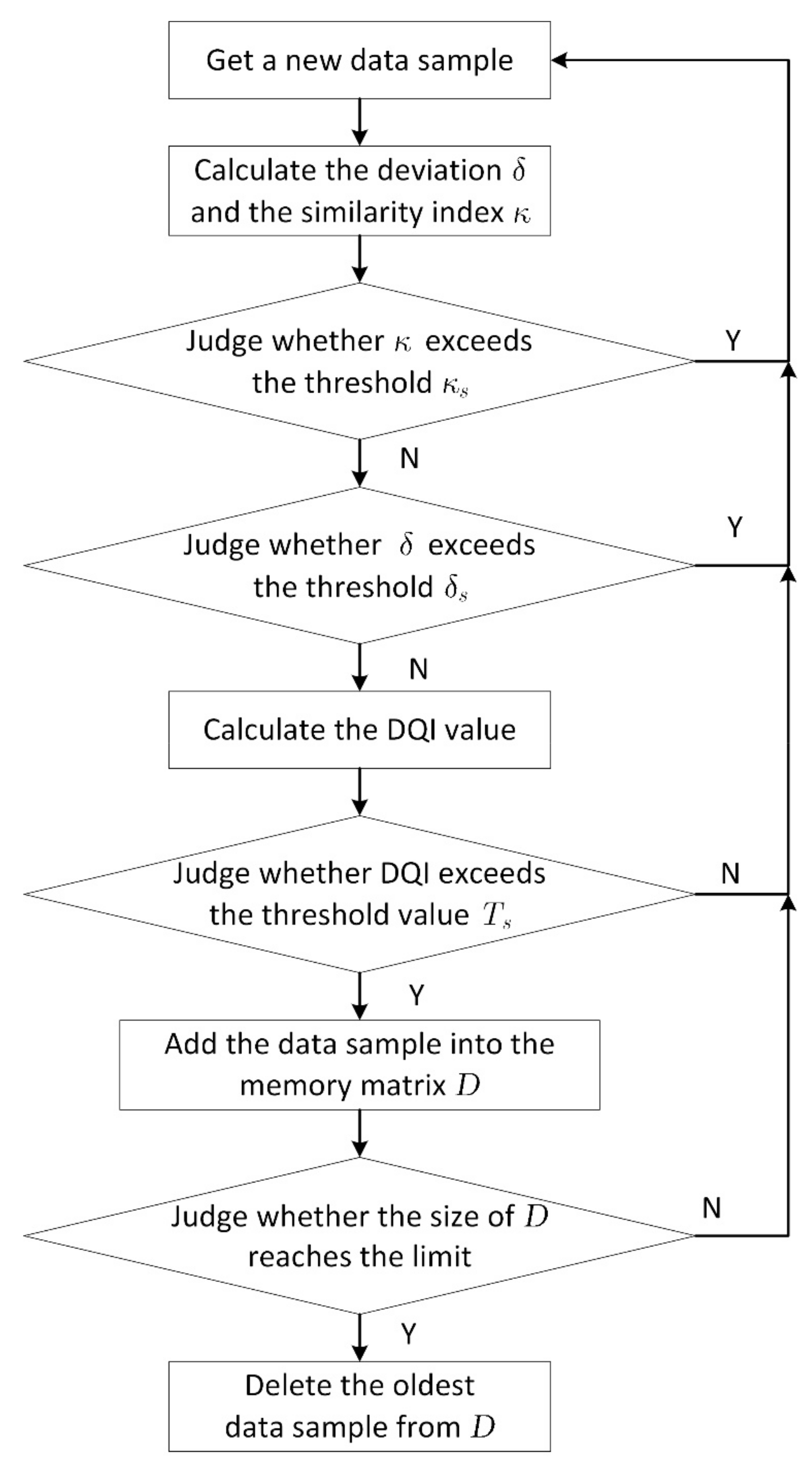
The estimation error, which is produced by the MSET model, can indicate the deviation between the current state from norm operations. Thus, in this study, the deviation ( δ ), which is the norm value of the residual, is utilized to identify early faults of ID fans. The deviation ( δ ) is calculated as follows:
δ x   =   i = 1 n x i x ^ i 2
where x ^ is the estimation of x , and it can be calculated by using Equation (11).
When the deviation ( δ ) is larger, the dissimilarity between the observation vector ( x ) and the estimation vector ( x ^ ) is higher. Based on the deviation, we define the similarity index ( κ ), which is limited to the range of 0 ,   1 , for better detection of ID fan faults.
κ x   =   1 i = 1 n μ i x i x ^ i 2 θ
where θ is a similarity threshold, μ i is the weight of the i th variable.
The weights μ i in Equation (13) can be determined based on the estimation residuals of samples in the validation set to remove the influence of error variations of different variables:
μ i = 1 / e i i = 1 n 1 / e i
where e i is the mean error of the i th variable in the prediction of the validation set.
The threshold θ in Equation (13) can set to be the upper limit of the confidence interval of the estimation residuals of the validation set with a level 1 α [29]:
θ = d ¯ + σ / N t α / 2 N 1
where d ¯ and σ are the mean and variance of the prediction residuals of the validation set, t α / 2 N 1 is the T-distribution with the confidence level 1 α , and N is the size of the validation dataset.
Equation (13) shows that if the equipment runs in normal operations, the estimation x ^ will have a high similarity to the observation x , and thus κ is close to 1. If the equipment runs in abnormal operations, the similarity will be beyond the normal range and κ is close to 0. Therefore, the similarity index can be taken as a visual indicator for fault judgment.
Moreover, the similarity value is easily influenced by the random disturbance. The moving window method is applied to optimize the similarity value. Considering a period of L data samples, the similarity sequences κ 1 , κ 2 , , κ T , κ L can be calculated by Equation (13). Assuming that the moving window width is T , the mean similarity value of each sub-window is obtained:
κ ¯ j = i = j T + j 1 κ i T
where j = 1 , 2 , , L T + 1 , which represents the similarity sequences index.
The warning threshold ( κ s ) can be set to the minimum of the similarity sequences multiplied by a coefficient:
κ s = γ min κ ¯ 1 , κ ¯ 2 ,   , κ ¯ t T + 1
where γ is a warning threshold coefficient, which can be adjust to guarantee that all the operations in the validation set are recognized to be normal; that is, the similarity sequence values are just above the threshold, κ s . Thus, A warning signal will be produced when the similarity of the current observation falls below the threshold, κ s .

2.4. MSET Update

The ID fan usually runs in variant conditions because of the environmental change and boiler load regulation. The MSET model trained with the memory matrix selected from certain operations fails to represent the whole characteristics of the ID fan. When it runs in a different operating condition, the observed value may quite differ from the data in the memory matrix, leading to inaccurate estimations. Thus, it is necessary to implement an update strategy to make the memory matrix cover new information to update the MSET model.
However, if all the newly acquired data are added into the memory matrix, the size of D will be constantly increased, leading to a heavy computation. Thus, the update strategy can be implemented incrementally. Once a new observation is obtained, it is analyzed to check whether it satisfies the updating criteria. If yes, then it is added into D ; and meanwhile, an old sample is selected and deleted from D to maintain the matrix size unchanged. After a new D is obtained, the MSET model is calculated accordingly.
The first step of the MSET update procedure is to check whether the newly acquired data sample belongs to normal operations. To achieve this, the similarity index ( κ ) is calculated according to Equations (11)–(15). If the similarity index ( κ ) exceeds the warning threshold ( κ s ), this sample is considered to reflect an abnormal behavior, and the next data sample is focused on; otherwise, its estimation deviation ( δ ) is analyzed next. If the deviation ( δ ) keeps in an instant growth, we believe that this data sample may be in the fault-development stage, and then the next data sample is focused on. If deviation ( δ ) is below a given deviation threshold ( δ s ), then we consider the sample as a totally normal operation, and the next step is to check whether this sample contains new operating information that is not covered by the memory matrix ( D ). The data quality index (DQI), which builds the relationship between the new data sample and the memory matrix, is defined to select the data sample that represents new operating information. The DQI is expressed as follows:
D Q I x o = i = 1 n x o i     x ¯ i i = 1 n x o i     x ¯ i 2
where x o i is the i th variable value in the new data sample, x ¯ i is the average value of the i th variable, n is the number of variables. The data sample with a large DQI is considered to help increase the operating information in D . A threshold ( T s ) is set to determine whether the data sample is added into D :
T s = max 1 j m i = 1 n x j i     x ¯ i i = 1 n x j i     x ¯ i 2
where n is the number of variables, and m is the number of data samples in D . If the DQI value of the new sample has a larger value than T s , it is added into D . Meanwhile, to keep the matrix size unchanged, the oldest data sample, which may have become invalid, is deleted from D .
The flowchart of the MSET update is shown in Figure 2. Firstly, a new data sample is acquired and focused on. The deviation ( δ ) and similarity index ( κ ) are calculated according to Equations (12) and (13), respectively. The value of the similarity index ( κ ) is judged, and if the similarity index ( κ ) exceeds the threshold ( κ s ), a new data sample is acquired. Otherwise, the value of the deviation ( δ ) is analyzed to determine whether the sample is in the fault-development stage. If the sample is identified to be in totally normal operation, the DQI value is calculated according to Equation (18). Then we check the DQI value according to the threshold ( T s ) to determine whether it is added into the memory matrix ( D ). Finally, the size of D  is checked, and if it reaches the limit, the oldest sample is deleted.

3. Industrial Case Study

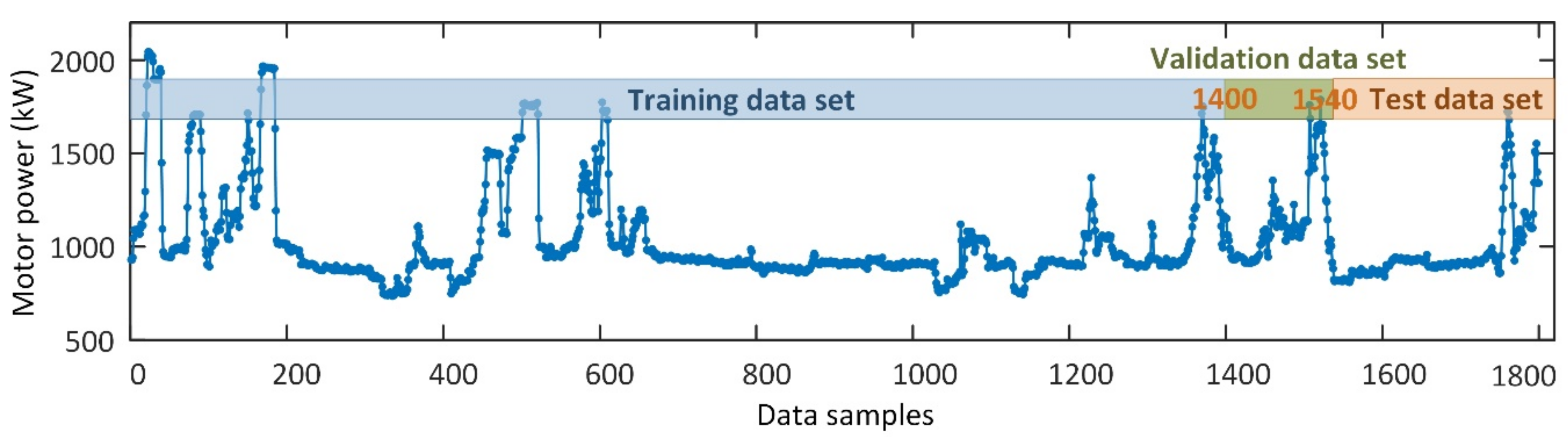
3.1. Data Preparation

The operating data of the ID fan are acquired from the plant-level supervisory information system (SIS) in a 300 MW coal-fired power station. More than 20 parameters related to the ID fan operation are recorded in the database, but only 7 fault-sensitive parameters are selected as the feature variables to develop the MSET model. These parameters specifically consist of motor power, an output pressure, a bearing temperature at the fan drive end (FDE), horizontal and vertical vibrations at the FDE, and horizontal and vertical vibrations at the fan non-drive end (FNDE). The real-time operating information of these parameters is recorded in the SIS; thus, the data can be mined to recognize early faults of the ID fan. The measurement locations of the mentioned parameters are shown in Figure 3, and their normal operating ranges are illustrated in Table 1.
Nearly two weeks of operating data of the ID fan system are acquired from the plant-level SIS database with a resolution of 10 min, with total 1800 samples. At the 1560th data sample, a cumulative deviation with a step length of 0.06 is artificially added to the FDE bearing temperature to simulate the abnormal temperature state caused by the fault of the induced draft fan. The first 1400 samples are considered as the available training dataset to construct the memory matrix ( D ) and develop the MSET model. The next 140 samples form a validation dataset to evaluate the prediction accuracy of the MSET model on the normal operations; in addition, the validation dataset is also used to determine the parameters related to the fault detection strategy, including the deviation threshold ( δ s ), the similarity threshold θ , weights ( μ i ), the warning threshold coefficient ( γ ), etc. Both the training and validation data are obtained during normal operation. The remaining 260 samples cover the span from normal operation to fault occurring are considered as the test dataset to verify the fault-detection performance of the model. The partition of the training dataset, validation dataset, and test dataset is shown in Figure 4.
In addition, three criteria are used to evaluate the prediction accuracy of models M1 and M2, i.e., the root mean squared errors (RMSE), normalized root mean squared error (NRMSE), and mean absolute error (MAE), which can be calculated as follows:
RMSE = 1 n i = 1 n x ^ i x i 2
NRMSE = RMSE x m a x x m i n × 100 %
MAE = 1 n i = 1 n x ^ i x i
where x i is the measured value at time stamp i , x ^ i is its estimation, and n is the number of data samples.

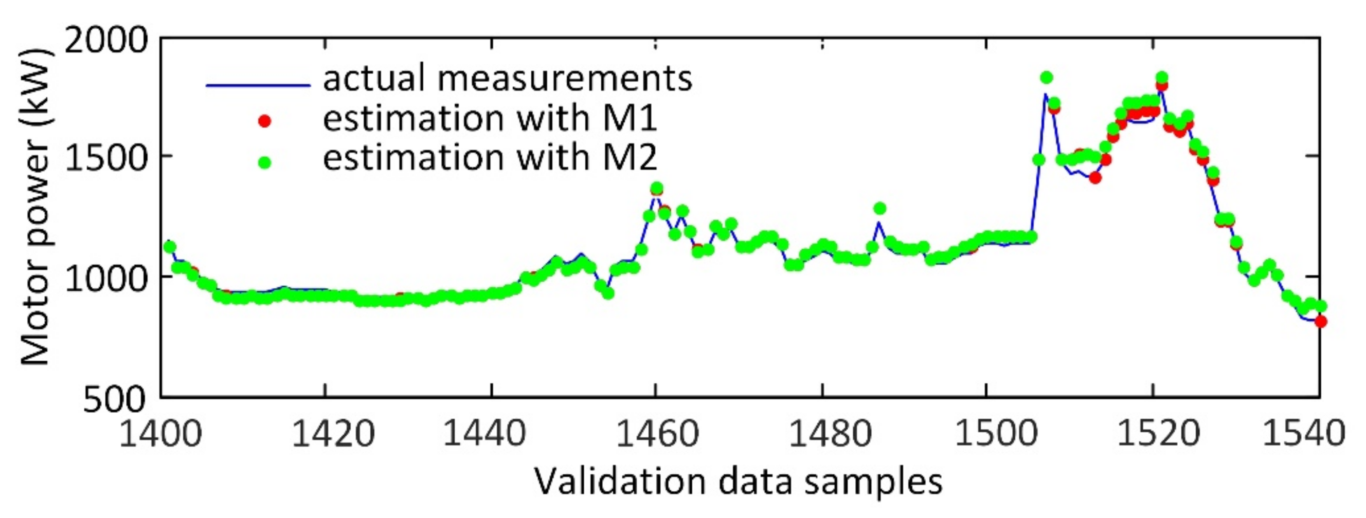
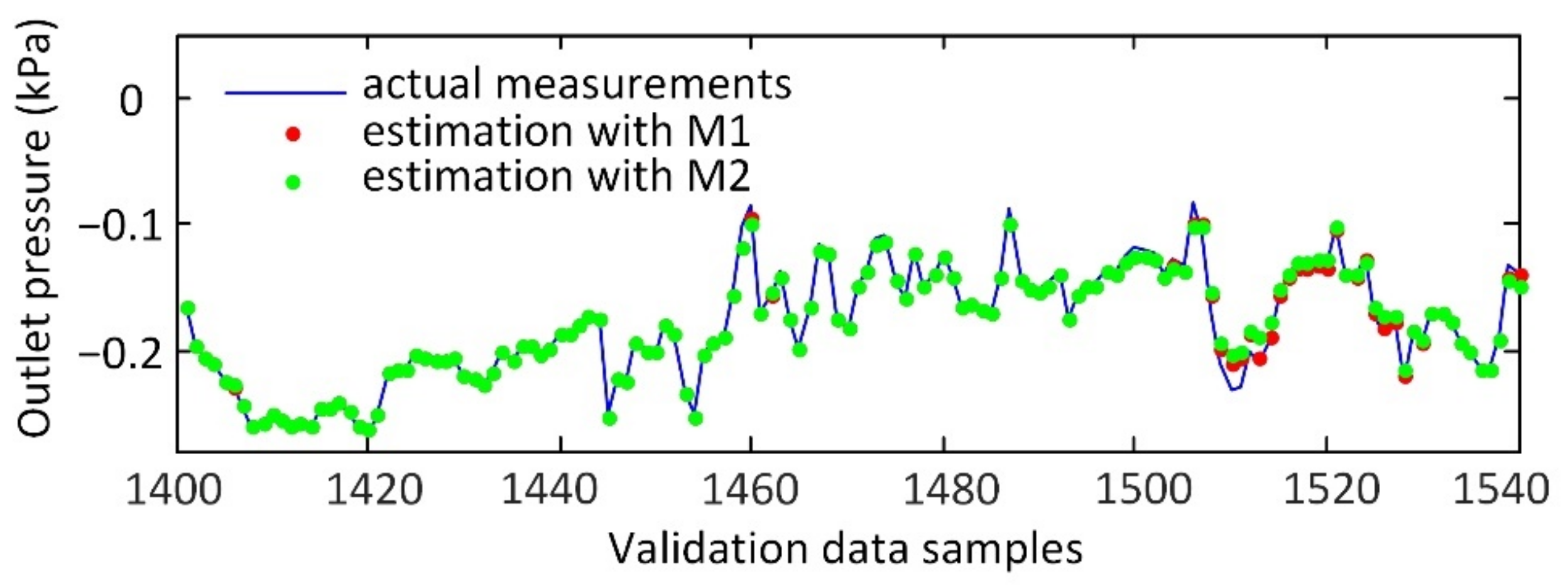
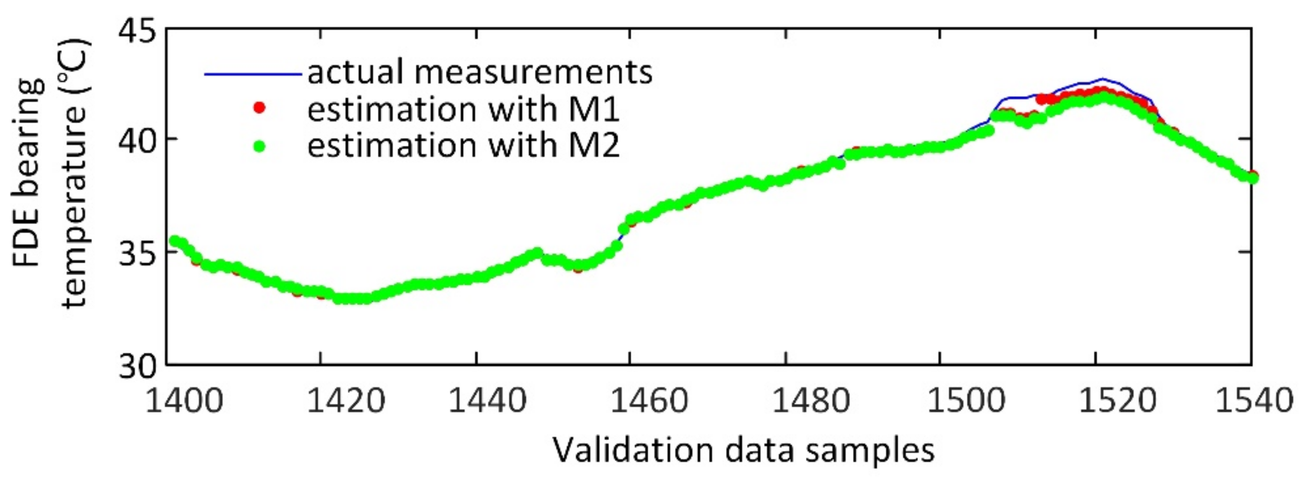
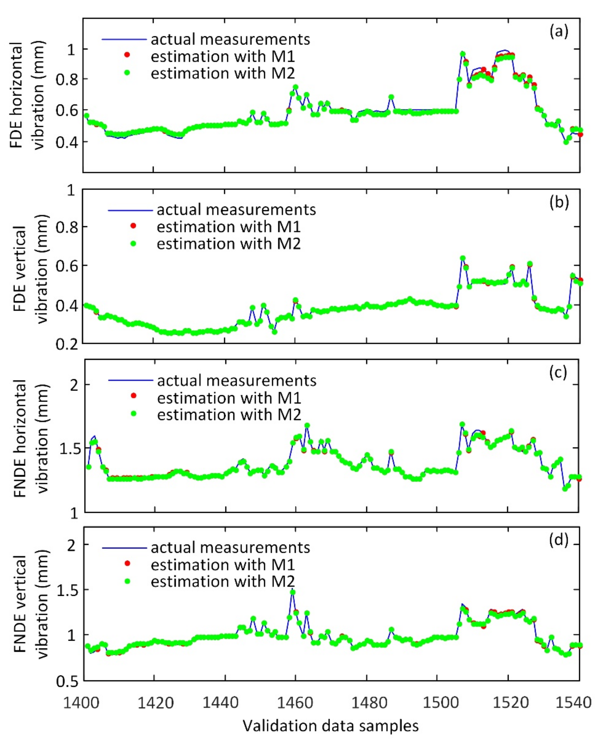
3.2. Modeling Results and Discussion

The memory matrix ( D ) is designed to consist of 200 samples, which are selected according to a well-designed criterion. The MSET model was developed based on Equations (1)–(11). To validate the proposed update strategy, two models were constructed: the MSET with adaptive update strategy (denoted as M1) and the MSET model without update (denoted as M2). The prediction results of the validation dataset are calculated by using models M1 and M2. During the prediction of model M1, the estimation result of the new data sample in the validation dataset is analyzed to determine whether it is added into the memory matrix ( D ) according to the update strategy. The data samples in D are updated when the new operating condition occurs. However, during the prediction of model M2, the estimation results are calculated without such an update procedure.
Figure 5 gives the estimations and actual measured values of the motor power by using models M1 and M2. The estimations are basically coincident with actual measured values of the motor power from the 1401st to the 1510th data samples. Furthermore, the estimations produced by model M1 are much closer to the measured values of the motor power from the 1511th to the 1540th data samples.
The detailed estimation errors of the motor power are given in Table 2. It is shown that models M1 and M2 produce almost the same-level estimation errors from the 1401st to the 1510th data samples. For example, the RMSE values of the two models are 26.2 and 31.8 kW, respectively. However, from the 1511th to the 1540th data samples, the estimation errors of model M1 are much lower than those of model M2. The RMSE of motor power predicted by M2 is 50.0 kW, but the RMSE produced by model M1 is only 32.9 kW, about 34.2% reduced. Thus, one can find that the prediction accuracy is greatly improved after the proposed update strategy is implemented.
Similar results can be obtained when using models M1 and M2 to predict the outlet pressure in the validation dataset, and these results are illustrated in Figure 6 and Table 3. The two models exhibit similar accuracy during the prediction from the 1401st to the 1510th data samples. For example, the NRMSE values of models M1 and M2 are 2.44% and 2.77%, respectively. From the 1510th data sample, a small deviation between the estimation and actual measured values occurs for both two models, but overall, model M1 produces a much more accurate prediction. From the 1511th to 1540th data samples, model M1 produces an NRMSE value of 4.33%, whereas the NRMSE of model M2 drops to 6.92%. It indicates that the memory matrix of model M1 covers new operating conditions after the update, and thus the prediction accuracy is improved.
Figure 7 and Table 4 show the prediction results of FDE bearing temperature. The estimations of the two models are basically the same except for the 1515th to the 1525th data samples, where the estimations produced by model M1 are closer to approaching the actual measured values.
The estimation results of the vibrations are shown in Figure 8 and Table 5, Table 6, Table 7 and Table 8. The estimations of the two models M1 and M2 are generally close to actual measured values, but the estimations of some samples produced by model M1 are more accurate than those produced by model M2. For the FDE horizontal vibration (see Figure 8a and Table 5), the estimation errors of model M1 are smaller than those of model M2 around the 1515th and the 1520th data samples. The RMSE values of models M1 and M2 during the prediction from 1511th to 1540th data samples are 0.018 and 0.023, respectively. The NRMSE and MAE values of model M1 are also smaller than those of model M2. Thus, we can find that the proposed update strategy is beneficial to improve prediction accuracy. We only analyzed the variable of FDE horizontal vibration, and the accuracy improvement of model M1 is still valid to other vibration variables.
Same results are obtained during the prediction of the FDE vertical vibration (see Figure 8b and Table 6), the FNDE horizontal vibration (see Figure 8c and Table 7), and the FNDE vertical vibration (see Figure 8d and Table 8). For the FDE vertical vibration (see Figure 8b), models M1 and M2 produce almost identical estimations; for the FNDE horizontal vibration (see Figure 8c), model M1 has lower estimation errors than model M2 when predicting the 1515th data sample; for the FNDE vertical vibration (see Figure 8d), the estimations of model M1 are closer to actual measurements around the 1520th data sample.

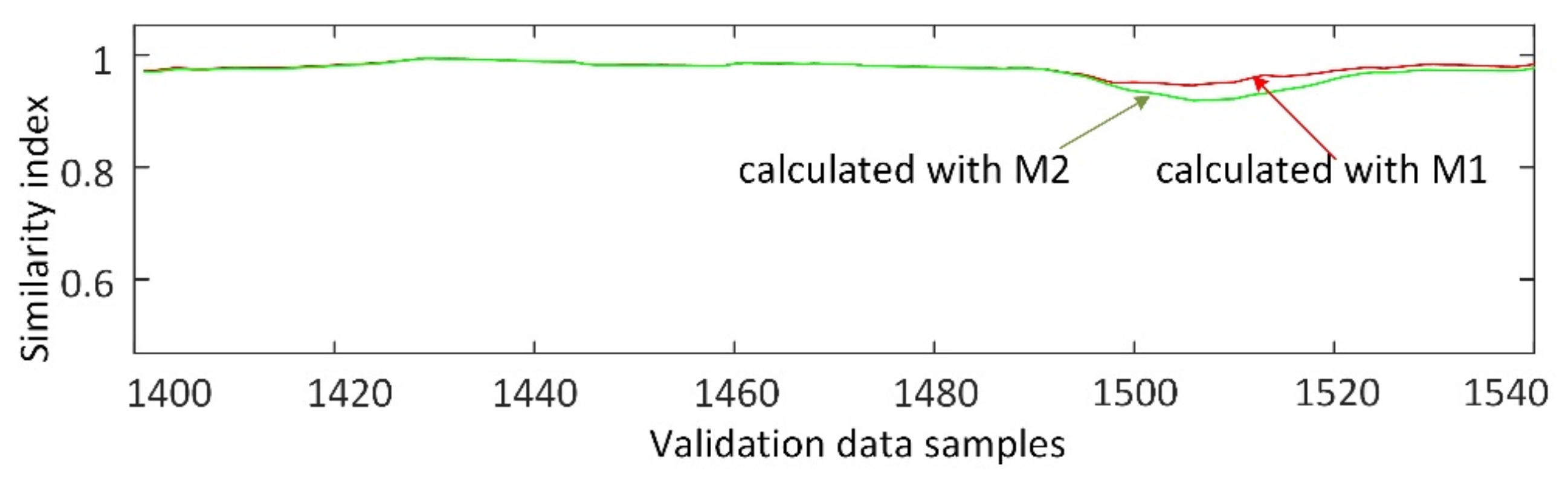
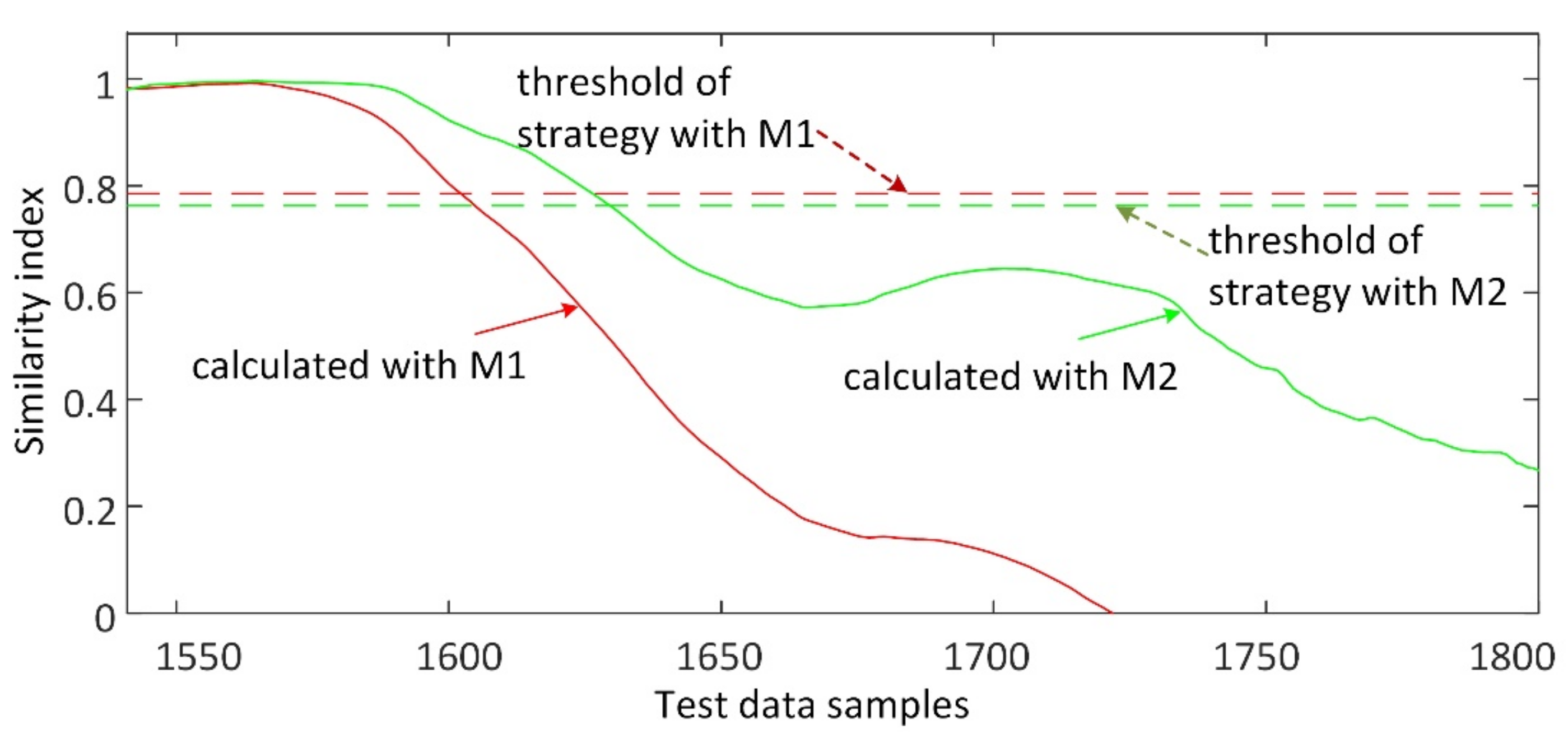
3.3. Fault Detection Based on Similarity Index

Considering the estimations of all the feature variables, the similarity index of the validation dataset can be calculated by Equation (13), and the results are shown in Figure 9. It can be found that the similarity index values calculated by models M1 and M2 generally coincide from the 1401st to the 1497th data samples. The similarity index of model M1 is much closer to 1.0 than that of model M2 after the 1498th data sample. According to the prediction results of the validation dataset, the warning threshold coefficient, γ , is set to 0.83, and the fault warning thresholds of models M1 and M2 are respectively 0.79 and 0.76. The similar index values of models M1 and M2 during the validation dataset show that model M1 can achieve better estimation than model M2 during normal operation.
The test dataset, which consists of 260 data samples (from the 1541st data sample to the 1800th data sample), was used to evaluate the fault-detection performance of the proposed model. The similarity index values of the test dataset were calculated by using models M1 and M2, and the results are shown in Figure 10. The similarity index values calculated by the two models show a general downward trend. The similarity index of model M1 drops from 0.98 to 0, and the similarity index of model M2 drops from 0.98 to 0.27. Thus, both two models can capture the abnormal increasing trend of the FDE bearing temperature. In addition, the similarity index calculated by model M1 decreases at a faster rate compared with model M2. The similarity index of model M1 decreases to the warning threshold of 0.79 after the 1602nd data sample, indicating that an abnormal operation is identified. The similarity index of model M2 reaches the warning threshold of 0.76 after the 1630th data sample. Thus, one can find that model M1 can detect the abnormality of the ID fan 28 data points (i.e., 4 h and 40 min) earlier than model M2, which indicates that the proposed adaptive update strategy is beneficial to advance the fault warning time.

4. Conclusions

In this paper, an adaptive early fault detection strategy was proposed for the ID fans in coal-fired power plants based on the MSET model. Firstly, the informative memory matrix was selected from historical normal operating data to construct the offline MSET model. The prediction deviations were taken as the inputs to define a similarity index that represents the operating status of the ID fan. Then, in order to deal with the problem of variant condition operation of the ID fan, an online update strategy was implemented based on monitoring the DQI of the operating data to make the memory matrix cover new information and update the MSET model. The proposed strategy was applied to an ID fan in a 300 MW coal-fired power plant for fault detection. The performance was compared with the model without an update.
First, the prediction results of the validation dataset show that the MSET model with the online update has better accuracy than the model without updates, which means that the proposed update strategy is beneficial to enhance the monitoring accuracy during the normal operation of the ID fan. Second, the fault-detection results of the test dataset show that the adaptive early fault detection model is more sensitive to the fault of the ID fan and can achieve an earlier warning than the model without updates. Finally, the proposed method is not only applicable to ID fans, but also to other industrial processes where a certain relationship exists among the feature variables.
In addition, the proposed method was verified by using the real operating data of the ID fan from a coal-fired power plant; however, there are still a series of complex problems to be solved before its practical application. In view of not affecting the power generation process of the power plant, a feasible solution is to package the proposed model into a dynamic link library and integrate it within the supervisory platform of the power plant to realize practical application, which will be our future work.

Author Contributions

Conceptualization, methodology, R.G. and G.Z.; software, validation, formal analysis, M.L. and Y.L.; investigation, resources, data curation, Q.Z. and L.Z.; writing—original draft preparation, M.L. and Y.L.; writing—review and editing, Y.L.; visualization, supervision, project administration, H.Y.; funding acquisition, R.G. and G.Z. All authors have read and agreed to the published version of the manuscript.

Funding

This research was funded by Major Science and Technology Projects of the Inner Mongolia Autonomous Region, grant number 2021-677, and National Natural Science Foundation of China, grant number 52061635102.

Institutional Review Board Statement

Not applicable.

Informed Consent Statement

Not applicable.

Data Availability Statement

Data is contained within the article.

Conflicts of Interest

The authors declare no conflict of interest.

References

  1. Wang, Y.; Tan, H.; Dong, K.; Liu, H.; Xiao, J.; Zhang, J. Study of ash fouling on the blade of induced fan in a 330 MW coal-fired power plant with ultra-low pollutant emission. Appl. Therm. Eng. 2017, 118, 283–291. [Google Scholar] [CrossRef]
  2. Du, J.; Liang, J.; Zhang, L. Research on the failure of the induced draft fan’s shaft in a power boiler. Case Study Eng. Fail. Anal. 2016, 5–6, 51–58. [Google Scholar] [CrossRef] [Green Version]
  3. Wei, Y.; Li, Y.; Xu, M.; Huang, W. A Review of Early Fault Diagnosis Approaches and Their Applications in Rotating Machinery. Entropy 2019, 21, 409. [Google Scholar] [CrossRef] [PubMed] [Green Version]
  4. Aguilar, J.; Garces, A.; Avendaño, A.; Macias, F.; White, C.; Gomez-Pulido, J.; De Mesa, J.G.; Garces-Jimenez, A. An Autonomic Cycle of Data Analysis Tasks for the Supervision of HVAC Systems of Smart Building. Energies 2020, 13, 3103. [Google Scholar] [CrossRef]
  5. Liu, J.; Bai, M.; Long, Z.; Liu, J.; Ma, Y.; Yu, D. Early Fault Detection of Gas Turbine Hot Components Based on Exhaust Gas Temperature Profile Continuous Distribution Estimation. Energies 2020, 13, 5950. [Google Scholar] [CrossRef]
  6. Cong, X.; Zhang, C.; Jiang, J.; Zhang, W.; Jiang, Y.; Zhang, L. A Comprehensive Signal-Based Fault Diagnosis Method for Lithium-Ion Batteries in Electric Vehicles. Energies 2021, 14, 1221. [Google Scholar] [CrossRef]
  7. Zhang, M.; Wang, T.Z.; Tang, T.T.; Liu, Z.; Claramunt, C. A Synchronous Sampling Based Harmonic Analysis Strategy for Marine Current Turbine Monitoring System under Strong Interference Conditions. Energies 2019, 12, 2117. [Google Scholar] [CrossRef] [Green Version]
  8. Shen, C.; Xie, J.; Wang, D.; Jiang, X.; Shi, J.; Zhu, Z. Improved Hierarchical Adaptive Deep Belief Network for Bearing Fault Diagnosis. Appl. Sci. 2019, 9, 3374. [Google Scholar] [CrossRef] [Green Version]
  9. Wang, H.; Wang, H.; Jiang, G.; Li, J.; Wang, Y. Early Fault Detection of Wind Turbines Based on Operational Condition Clustering and Optimized Deep Belief Network Modeling. Energies 2019, 12, 984. [Google Scholar] [CrossRef] [Green Version]
  10. Pozo, F.; Vidal, Y. Wind Turbine Fault Detection through Principal Component Analysis and Statistical Hypothesis Testing. Energies 2016, 9, 3. [Google Scholar] [CrossRef] [Green Version]
  11. Dai, J.; Tang, J.; Shao, F.; Huang, S.; Wang, Y. Fault Diagnosis of Rolling Bearing Based on Multiscale Intrinsic Mode Function Permutation Entropy and a Stacked Sparse Denoising Autoencoder. Appl. Sci. 2019, 9, 2743. [Google Scholar] [CrossRef] [Green Version]
  12. Kim, I.; Kim, W. Development and Validation of a Data-Driven Fault Detection and Diagnosis System for Chillers Using Machine Learning Algorithms. Energies 2021, 14, 1945. [Google Scholar] [CrossRef]
  13. Xiao, Y.; Pan, W.; Guo, X.; Bi, S.; Feng, D.; Lin, S. Fault Diagnosis of Traction Transformer Based on Bayesian Network. Energies 2020, 13, 4966. [Google Scholar] [CrossRef]
  14. Shin, J.-H.; Kim, J.-O. On-Line Diagnosis and Fault State Classification Method of Photovoltaic Plant. Energies 2020, 13, 4584. [Google Scholar] [CrossRef]
  15. Zhou, Y.; Yang, X.; Tao, L.; Yang, L. Transformer Fault Diagnosis Model Based on Improved Gray Wolf Optimizer and Probabilistic Neural Network. Energies 2021, 14, 3029. [Google Scholar] [CrossRef]
  16. Suh, S.; Lee, H.; Jo, J.; Lukowicz, P.; Lee, Y.O. Generative Oversampling Method for Imbalanced Data on Bearing Fault Detection and Diagnosis. Appl. Sci. 2019, 9, 746. [Google Scholar] [CrossRef] [Green Version]
  17. Vidal, Y.; Pozo, F.; Tutivén, C. Wind Turbine Multi-Fault Detection and Classification Based on SCADA Data. Energies 2018, 11, 3018. [Google Scholar] [CrossRef] [Green Version]
  18. Guo, Z.; Liu, M.; Qin, H.; Li, B. Mechanical Fault Diagnosis of a DC Motor Utilizing United Variational Mode Decomposition, SampEn, and Random Forest-SPRINT Algorithm Classifiers. Entropy 2019, 21, 470. [Google Scholar] [CrossRef] [PubMed] [Green Version]
  19. Gross, K.C.; Singer, R.M.; Wegerich, S.W.; Herzog, J.P. Application of a model-based fault detection system to nuclear plant signals. In Proceedings of the 9th International Conference on Intelligent Systems Application to Power System, Seoul, Korea, 6–10 July 1997; pp. 212–218. [Google Scholar]
  20. Caesarendra, W.; Lee, J.M.; Ha, J.M.; Choi, B.K. Slew Bearing Early Damage Detection Based on Multivariate State Estimation Technique and Sequential Probability Ratio Test. In Proceedings of the IEEE/ASME International Conference on Advanced Intelligent Mechatronics (AIM), Busan, Korea, 7–11 July 2015; pp. 1161–1166. [Google Scholar]
  21. Guo, P.; Bai, N. Wind Turbine Gearbox Condition Monitoring with AAKR and Moving Window Statistic Methods. Energies 2011, 4, 2077–2093. [Google Scholar] [CrossRef] [Green Version]
  22. Zhang, W.; Liu, J.; Gao, M.; Pan, C.; Huusom, J.K. A fault early warning method for auxiliary equipment based on multivariate state estimation technique and sliding window similarity. Comput. Ind. 2019, 107, 67–80. [Google Scholar] [CrossRef]
  23. Cui, C.; Lin, W.; Yang, Y.; Kuang, X.; Xiao, Y. A novel fault measure and early warning system for air compressor. Measurement 2019, 135, 593–605. [Google Scholar] [CrossRef]
  24. Wang, Z.; Liu, C. Wind turbine condition monitoring based on a novel multivariate state estimation technique. Measurement 2021, 168. [Google Scholar] [CrossRef]
  25. Long, D.; Zheng, H.; Hong, F. Condition Monitoring of Industrial Equipment Based on Multi-Variables State Estimate Technique. Appl. Sci. 2020, 10, 5637. [Google Scholar] [CrossRef]
  26. Caesarendra, W.; Tjahjowidodo, T.; Kosasih, B.; Tieu, A.K. Integrated Condition Monitoring and Prognosis Method for Incipient Defect Detection and Remaining Life Prediction of Low Speed Slew Bearings. Machines 2017, 5, 11. [Google Scholar] [CrossRef] [Green Version]
  27. Lv, Y.; Fang, F.; Yang, T.T.; Liu, J.Z. An early fault detection method for induced draft fans based on MSET with informative memory matrix selection. ISA Trans. 2020, 102, 325–334. [Google Scholar] [CrossRef]
  28. Guo, P.; Infield, D.; Yang, X. Wind turbine generator condition-monitoring using temperature trend analysis. IEEE Trans. Sustain. Energy 2012, 3, 124–133. [Google Scholar] [CrossRef] [Green Version]
  29. Wang, Y.; Infield, D. Supervisory control and data acquisition data-based non-linear state estimation technique for wind turbine gearbox condition monitoring. IET Renew. Power Gener. 2013, 7, 350–358. [Google Scholar] [CrossRef]
  30. Xu, G.; Guo, W.; Zhao, Y.; Zhou, Y.; Zhang, Y.; Liu, X.; Xu, G.; Li, G. Online Learning Based Underwater Robotic Thruster Fault Detection. Appl. Sci. 2021, 11, 3586. [Google Scholar] [CrossRef]
  31. Liu, W.; Ran, W.; Nantogma, S.; Xu, Y. Adaptive Information Sharing with Ontological Relevance Computation for Decentralized Self-Organization Systems. Entropy 2021, 23, 342. [Google Scholar] [CrossRef]
  32. Chen, X.; Liu, Z.; Wang, J.; Yang, C.; Long, B.; Zhou, X. An Adaptive Prediction Model for the Remaining Life of an Li-Ion Battery Based on the Fusion of the Two-Phase Wiener Process and an Extreme Learning Machine. Electronics 2021, 10, 540. [Google Scholar] [CrossRef]
  33. Kadlec, P.; Grbić, R.; Gabrys, B. Review of adaptation mechanisms for data-driven soft sensors. Comput. Chem. Eng. 2011, 35. [Google Scholar] [CrossRef]
  34. Liu, Y.; Gao, Z.; Li, P.; Wang, H. Just-in-time kernel learning with adaptive parameter selection for soft sensor modeling of batch processes. Ind. Eng. Chem. Res. 2012, 51, 4313–4327. [Google Scholar] [CrossRef]
  35. Shi, H.; Guo, J.; Bai, X.; Guo, L.; Liu, Z.; Sun, J. Research on a Nonlinear Dynamic Incipient Fault Detection Method for Rolling Bearings. Appl. Sci. 2020, 10, 2443. [Google Scholar] [CrossRef] [Green Version]
  36. Ammiche, M.; Kouadri, A.; Bensmail, A. A modified moving window dynamic PCA with Fuzzy Logic Filter and application to fault detection. Chemom. Intell. Lab. Syst. 2018, 177, 100–113. [Google Scholar] [CrossRef]
  37. Sheriff, M.Z.; Mansouri, M.; Karim, M.N.; Nounou, H.; Nounou, M. Fault detection using multiscale PCA-based moving window GLRT. J. Process Control 2017, 54, 47–64. [Google Scholar] [CrossRef]
  38. Chen, K.; Liang, Y.; Gao, Z.; Liu, Y. Just-in-Time Correntropy Soft Sensor with Noisy Data for Industrial Silicon Content Pre-diction. Sensors 2017, 17, 1830. [Google Scholar] [CrossRef] [Green Version]
  39. Ahmad, I.; Ayub, A.; Mohammad, N.; Kano, M. Data-Based Prediction and Stochastic Analysis of Entrained Flow Coal Gasification under Uncertainty. Sensors 2019, 19, 1626. [Google Scholar] [CrossRef] [Green Version]
  40. Jiang, J.; Xiao, Z.; Wang, J.; Song, J. Sequential Method with Incremental Analysis Update to Retrieve Leaf Area Index from Time Series MODIS Reflectance Data. Remote Sens. 2014, 6, 9194–9212. [Google Scholar] [CrossRef] [Green Version]
  41. Kaneko, H.; Funatsu, K. Adaptive database management based on the database monitoring index for long-term use of adaptive soft sensors. Chemom. Intell. Lab. Syst. 2015, 146, 179–185. [Google Scholar] [CrossRef] [Green Version]
  42. Lv, Y.; Lv, X.; Fang, F.; Yang, T.; Romero, C.E. Adaptive Selective Catalytic Reduction Model Development Using Typical Operating Data in Coal-Fired Power Plants. Energy 2020, 192, 116589. [Google Scholar] [CrossRef]
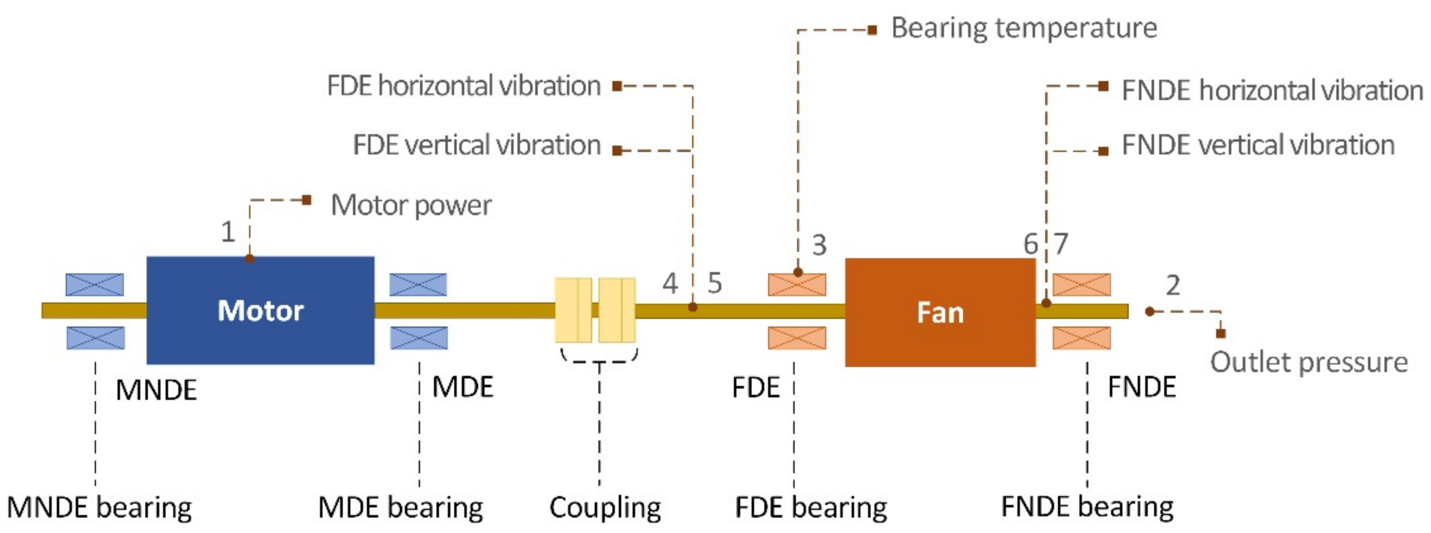
Figure 1. Framework of the adaptive early fault detection model.
Energies 14 04787 g001
Figure 2. Memory matrix update procedure.
Energies 14 04787 g002
Figure 3. Measurement locations of the parameters of the ID fan.
Energies 14 04787 g003
Figure 4. The division of training dataset, validation dataset, and test dataset.
Energies 14 04787 g004
Figure 5. Estimation of motor power in validation dataset by using models M1 and M2.
Energies 14 04787 g005
Figure 6. Estimation of outlet pressure in validation dataset by using models M1 and M2.
Energies 14 04787 g006
Figure 7. Estimation of motor power in validation dataset by using models M1 and M2.
Energies 14 04787 g007
Figure 8. Estimation results of validation dataset by using models M1 and M2: (a) FDE horizontal vibration, (b) FDE vertical vibration, (c) FNDE horizontal vibration, and (d) FNDE vertical vibration.
Energies 14 04787 g008
Figure 9. Similarity index values of the validation dataset.
Energies 14 04787 g009
Figure 10. Similarity index values of the test dataset.
Energies 14 04787 g010
Table 1. Normal operating range of parameters related to the ID fan.
VariablesMeasurement LocationUnitOperating Range
Motor power1kW730~2050
Outlet pressure2kPa−0.33~−0.03
FDE bearing temperature3°C32.2~42.7
FDE horizontal vibration4mm0.21~1.30
FDE vertical vibration5mm0.21~1.30
FNDE horizontal vibration6mm0.75~2.05
FNDE vertical vibration7mm0.75~2.05
Table 2. Estimation errors of the motor power in validation dataset.
ModelsFrom 1401th to 1510th
Data Samples
From 1511th to 1540th
Data Samples
Entire Validate Dataset
RMSE
(kW)
NRMSE
(%)
MAE
(kW)
RMSE
(kW)
NRMSE
(%)
MAE
(kW)
RMSE
(kW)
NRMSE
(%)
MAE
(kW)
M124.02.8319.832.93.3823.0 26.22.6920.5
M224.62.9020.550.05.1440.031.83.2724.7
Table 3. Estimation errors of the outlet pressure in validation dataset.
ModelsFrom 1401th to 1510th
Data Samples
From 1511th to 1540th
Data Samples
Entire Validate Dataset
RMSE
(kPa)
NRMSE
(%)
MAE
(kPa)
RMSE
(kPa)
NRMSE
(%)
MAE
(kPa)
RMSE
(kPa)
NRMSE
(%)
MAE
(kPa)
M10.00452.440.00240.00554.330.00290.00472.570.0025
M20.00502.770.00260.00886.920.00550.00603.320.0032
Table 4. Estimation errors of FDE bearing temperature in validation dataset.
ModelsFrom 1401th to 1510th
Data Samples
From 1511th to 1540th
Data Samples
Entire Validate Dataset
RMSE
(°C)
NRMSE
(%)
MAE
(°C)
RMSE
(°C)
NRMSE
(%)
MAE
(°C)
RMSE
(°C)
NRMSE
(%)
MAE
(°C)
M10.161.780.100.378.630.290.222.230.14
M20.181.930.100.6013.920.490.323.170.19
Table 5. Estimation errors of the FDE horizontal vibration in validation dataset.
ModelsFrom 1401th to 1510th
Data Samples
From 1511th to 1540th
Data Samples
Entire Validate Dataset
RMSE
(mm)
NRMSE
(%)
MAE
(mm)
RMSE
(mm)
NRMSE
(%)
MAE
(mm)
RMSE
(mm)
NRMSE
(%)
MAE
(mm)
M10.0132.30.0110.0183.00.0130.0142.40.011
M20.0142.40.0110.0234.00.0170.0162.80.012
Table 6. Estimation errors of the FDE vertical vibration in validation dataset.
ModelsFrom 1401th to 1510th
Data Samples
From 1511th to 1540th
Data Samples
Entire Validate Dataset
RMSE
(mm)
NRMSE
(%)
MAE
(mm)
RMSE
(mm)
NRMSE
(%)
MAE
(mm)
RMSE
(mm)
NRMSE
(%)
MAE
(mm)
M10.0040.90.0020.0083.00.0070.0051.20.003
M20.0040.90.0020.0093.20.0080.0051.30.004
Table 7. Estimation errors of the FNDE horizontal vibration in validation dataset.
ModelsFrom 1401th to 1510th
Data Samples
From 1511th to 1540th
Data Samples
Entire Validate Dataset
RMSE
(mm)
NRMSE
(%)
MAE
(mm)
RMSE
(mm)
NRMSE
(%)
MAE
(mm)
RMSE
(mm)
NRMSE
(%)
MAE
(mm)
M10.0081.70.0050.0143.10.0110.0101.9 0.006
M20.0081.80.0050.0163.50.0130.0102.00.007
Table 8. Estimation errors of the FNDE vertical vibration in validation dataset.
ModelsFrom 1401th to 1510th
Data Samples
From 1511th to 1540th
Data Samples
Entire Validate Dataset
RMSE
(mm)
NRMSE
(%)
MAE
(mm)
RMSE
(mm)
NRMSE
(%)
MAE
(mm)
RMSE
(mm)
NRMSE
(%)
MAE
(mm)
M10.0111.50.0060.0122.40.0090.0111.60.007
M20.0131.70.0070.0173.40.0140.0141.90.009
Publisher’s Note: MDPI stays neutral with regard to jurisdictional claims in published maps and institutional affiliations.

