Optimal PMU Placement Technique to Maximize Measurement Redundancy Based on Closed Neighbourhood Search

Abstract

This paper proposes a method for the optimal placement of phasor measurement units (PMUs) for the complete observability of a power system based on the degree of the neighbourhood vertices. A three-stage algorithm is used to determine the minimum number of PMUs needed to make the system observable. The key objective of the proposed methodology is to minimize the total number of PMUs to completely observe a power system network and thereby minimize the installation cost. In addition, the proposed technique also focuses on improving the measurement redundancy. The proposed method is applied on standard IEEE 14-bus, IEEE 24-bus, IEEE 30-bus, IEEE 57-bus and IEEE 118-bus test systems and a hybrid AC/DC microgrid test system. The results obtained are compared with already existing methods in terms of the Bus Observability Index (BOI) and System Observability Redundancy Index (SORI). The results show that the proposed method is simple to implement and provides better placement locations for effective monitoring compared to other existing methods.

1. Introduction

The higher penetration levels of renewable power and the deregulation of the electricity sector to satisfy the ever-increasing demand for electricity are making the power system network more vulnerable. Hence, closely monitoring power grids is an important diagnostic task. This is effectively achieved by the deployment of Phasor Measurement Units (PMUs). PMUs have gained more popularity because of their ability to accurately measure bus voltage and branch current phasors with respect to a Global Positioning System (GPS) clock every few microseconds [1]. Placing PMUs at all locations in a power system network is not economically feasible due to their cost. Therefore, it is necessary to properly distribute PMUs in order to obtain a good estimation of power system states. This problem is known as an optimal PMU placement (OPP) problem. The preliminary objective of an OPP problem is to find strategic locations for PMU placement such that

• The system is completely observable and
• The solution is economically viable.

A power system is said to be completely observable only when all of its states can be uniquely determined [2]. Topological and numerical observability are the two different observabilities discussed in the literature. Algorithms to satisfy numerical observability demand many calculations and high precision related to cumulative error. However, algorithms that concentrate on addressing topological observability are simpler and are sufficient for the state estimator [3]. A major application of PMU is to improve state estimation [4]. This paper focuses on the optimal placement of PMUs from the perspective of state estimation. Hence, the discussions are limited to topological observability. Algorithms that deal with topological observability focus on the structural connectivity of the network.

Generally, deterministic approaches (such as integer programming [5,6,7,8,9,10,11,12,13,14] and the Groebner base algorithm [15]) and heuristic approaches are widely used to address topological observability. Dua et al. apply a multistage approach based on Integer Linear Programming (ILP). They also introduce two performance indices to measure the quality of measurement location selected [5]: the Bus Observability Index (BOI) and System Observability Redundancy Index (SORI). These indices are later used to evaluate the results obtained for the proposed method. However, it is known that deterministic approaches are influenced by the local minima, and integer programming cannot simultaneously handle multiple objectives such as minimizing the number of PMUs and maximizing the redundancy [16].

There are also a few contributions based on nature-inspired and evolutionary algorithms [17,18,19,20,21,22,23,24,25,26,27,28]. However, these solution methodologies are iterative and hence consume more computational time and space.

With regard to the analysis of the topology of a power system network, graph theoretical approaches are also followed in the literature. The paper by Baldwin et al. was one of the first of this kind to use graph theory for the OPP problem. The work explains the existence of local minima in the search space. To maximize the coverage, PMUs are placed at buses with the maximum degree [29]. However, it is proven that this may not result in the minimum number of PMUs because of the presence of local minima. Several methodologies involving graph theoretical concepts have been reported, and most of the work has focused on forming a spanning tree. Denegri et al. used a minimum spanning tree generation algorithm to locate optimal meter placement positions [30]. Haynes et al. introduced the power domination number to identify the location of measurement devices [31]. Nuqui et al. initially used the concept of a spanning tree and then used Simulated Annealing [32]. Venugopal et al. introduced the concepts of vertex colouring and the AVL tree to solve the optimal placement problem [33]. Recently, Devi et al. presented the genetic algorithm along with the concept of the minimum spanning tree [34]. Spanning tree approaches help researchers to arrive at a minimum number of PMUs but do not assure maximum redundancy.

Few works have reported on the concept of domination to identify the dominant set of the network. A multi-objective function that combines non-dominated sorting and the genetic algorithm has been used [35,36] to solve the optimization problem. Peng et al. combined non-dominated sorting with differential evolution [37]. Recently, Saravanan et al. used the concept of domination integrity [38]. It is inferred that, focusing on the non-dominating set, the authors arrived at a global optimal solution.

A bus is said to be directly observed if a PMU is placed at that bus and is said to be indirectly observed if a PMU is placed at its neighbouring bus. If all the buses in the network are either directly or indirectly observable, the network is said to be completely observable. The BOI and SORI act as indicators for observability and measurement redundancy [13]. By improving the measurement redundancy, poor-quality measurement data can be detected and removed by the bad data processor of the state estimator. In case of lower values of measurement redundancy, there may be critical measurements, and the loss of those measurements might affect the complete observability of the network. Furthermore, poor-quality data appearing in the critical measurements cannot be removed by the state estimator and will lead to the computation of an inaccurate estimation of the operating state of the power system [4]. Therefore, to improve the performance of state estimators, PMUs have to be placed tactically at locations to minimize their number and also maximize the coverage, thereby improving redundancy.

Comprehending the positive and negative aspects of various proposals, this paper uses graph theoretical concepts in three stages. In the first stage, a weight is introduced to minimize the number of PMUs and to maximize measurement redundancy. Based on this weight, the vertex set is divided into influential and non-influential subsets. The weight is calculated based on the degree of the vertex and the degree of its neighbouring vertices. In the second stage, by analyzing the elements of a non-influential subset, a few locations are selected. Finally, in the third stage, the set of locations selected in the previous stage is further reduced considering the BOI of every vertex. The obtained results are evaluated in terms of the BOI and SORI.

The paper is organized as follows: Section 2 delineates the technical background related to the proposed technique. Section 3 presents the problem formulation, highlighting the attributes that decide the optimal placement locations. Section 4 presents the solution methodology, explaining the three stages of the algorithm. Finally, Section 5 discusses the results and Section 6 concludes with the outcomes of the paper.

2. Technical Background

A graph $G=(V,E)$ consists of a set of objects $V=\{v_1,v_2,\dots ,v_n\}$ whose elements are called vertices and another set $E=\{e_1,e_2,\dots ,e_m\}$ whose elements are called edges, such that each edge $e_k$ is identified with an unordered pair $(v_i,v_j)$ of vertices [39]. Every power system network with buses $\{1,2,\dots ,n\}$ and transmission lines is modelled as a graph $G=(V,E)$ by replacing all buses with vertices $V=\{v_1,v_2,\dots ,v_n\}$ and edges $E=\{e_1,e_2,\dots ,e_m\}$.

Let $n=\left|V\right|$ and $m=\left|E\right|$ correspond to the cardinality of the vertex set and the edge set, respectively. Thus, n and m correspond to the number of buses and transmission lines of the power system network. If $e=(v_i,v_j)$, where $e\in E$ and $v_i,v_j\in V$, e is said to be incident with $v_i$ and $v_j$ (where $v_i$ and $v_j$ are called the end vertices of e). Furthermore, $v_i$ and $v_j$ are said to be adjacent to each other.

Let A be the adjacency matrix of the undirected graph G. Then,

$$A={\left[a_{ij}\right]}_{(n\times n)}$$

(1)

where

$$a_{ij}=\left\{\begin{array}{cc}1\hfill & \mathrm{if}{v}_i\mathrm{is}\mathrm{adjacent}\mathrm{to}{v}_j\hfill \\ 0\hfill & \mathrm{otherwise}\hfill \end{array}\right.$$

(2)

The open neighbourhood of the vertex $v_i$ is

$$N\left(v_i\right)=\{v_j\in V\left(G\right)/(v_i,v_j)\in E\left(G\right)\}$$

(3)

The closed neighbourhood of a vertex $v_i$ is

$$N\left[v_i\right]=\left\{v_i\right\}\bigcup N\left(v_i\right)$$

(4)

The degree of the vertex $v_i$, $d\left(v_i\right)$, is the cardinality of the open neighbourhood of $v_i$. Given a set of vertices $S=\{v_1,v_2,\dots ,v_x\}$, the open neighbourhood of S is

$$N\left(S\right)=N\left(v_1\right)\bigcup N\left(v_2\right)\bigcup \dots \bigcup N\left(v_x\right)$$

(5)

The closed neighbourhood of S is

$$N\left[S\right]=S\bigcup N\left(S\right)$$

(6)

In this paper, i or $v_i$ are interchangeably used to denote the bus i or vertex $v_i$.

3. Problem Formulation

The Optimal PMU Placement (OPP) problem is modelled as a cost-minimization problem. Let the binary variable $x_i$ denote the presence or absence of a PMU at bus $v_i$. Thus, PMU placement set for an n-bus system is

$$X=\{x_1,x_2,\dots ,x_n\}$$

(7)

where

$$x_i=\left\{\begin{array}{cc}1,\hfill & \mathrm{if}\mathrm{PMU}\mathrm{is}\mathrm{placed}\mathrm{at}\mathrm{bus}{v}_i\hfill \\ 0,\hfill & \mathrm{if}\mathrm{PMU}\mathrm{is}\mathrm{not}\mathrm{placed}\mathrm{at}\mathrm{bus}{v}_i\hfill \end{array}\right.$$

(8)

Let $w_i$ be the cost incurred for placing a PMU at bus $v_i$. The mathematical model of the OPP problem is

$$J=Min\sum _{i=1}^n{w}_i{x}_i$$

(9)

subject to $f_i\ge 1$, where $f_i$, the observability constraint of bus $v_i$, is given by

$$f_i=\sum _{j=1}^n{c}_{ij}{x}_j$$

(10)

where elements of the connectivity matrix are given by

$$c_{ij}=\left\{\begin{array}{cc}1,\hfill & \mathrm{if}i=j\mathrm{or}i\mathrm{is}\mathrm{adjacent}\mathrm{to}j\hfill \\ 0,\hfill & \mathrm{otherwise}\hfill \end{array}\right.$$

(11)

Given a graph G, OPP solution determines a set S such that every vertex of the system is in S or is the neighbour of the vertex in S. As, the vertex of S observes itself and all its neighbours [34], the diagonal elements of the connectivity matrix $c_{ii}$ are assigned a value of 1.

For an IEEE seven-bus system, the constraint function $f_i$ is described as

$$\left[\begin{array}{c}{f}_1\\ f_2\\ f_3\\ f_4\\ f_5\\ f_6\\ f_7\end{array}\right]=\left[\begin{array}{ccccccc}1& 1& 0& 0& 0& 0& 0\\ 1& 1& 1& 0& 0& 1& 0\\ 0& 1& 1& 1& 0& 1& 0\\ 0& 0& 1& 1& 1& 0& 1\\ 0& 0& 0& 1& 1& 0& 1\\ 0& 1& 1& 0& 0& 1& 0\\ 0& 0& 0& 1& 1& 0& 1\end{array}\right]\times \left[\begin{array}{c}{x}_1\\ x_2\\ x_3\\ x_4\\ x_5\\ x_6\\ x_7\end{array}\right]\ge \left[\begin{array}{c}1\\ 1\\ 1\\ 1\\ 1\\ 1\\ 1\end{array}\right]$$

(12)

That is, $f_i$ should hold a minimum value of 1 to satisfy complete observability and could correspond to a maximum value equal to 1 more than the degree of that vertex $v_i$; in other words, $1\le f_i\le d\left(v_i\right)+1$.

Hence, it could be concluded that the observability constraint is greatly influenced by the degree of the vertex. Along with the degree of the vertex, one more attribute, the average neighbourhood degree corresponding to the vertex, is considered. The average neighbourhood degree of a vertex $v_i$ is calculated by adding the degree of all vertices in the open neighbourhood of $v_i$ divided by the degree of that vertex $v_i$. The interlinking of the degree of the vertex with its average neighbourhood degree, $\gamma$, is calculated for every vertex. Thus, $\gamma \left(v_i\right)$ is the difference between the degree and the average neighbourhood degree of $v_i$. It is expressed mathematically as

$$\gamma \left(v_i\right)=d\left(v_i\right)-\frac{{\sum }_{v_j\in N\left(v_i\right)}d\left(v_j\right)}{d\left(v_i\right)}$$

(13)

The significance of the considered attributes (degree and average neighbourhood degree) is explained by considering the standard IEEE seven-bus system. The values are tabulated in

Table 1. Degree and average neighbourhood degree of IEEE seven-bus system.

Vertex	Degree	Average Neighbourhood Degree
$v_1$	1	3
$v_2$	3	2
$v_3$	3	2.667
$v_4$	3	2.333
$v_5$	2	2.5
$v_6$	2	3
$v_7$	2	2.5

.

From Table 1, it is observed that vertices $v_2$, $v_3$ and $v_4$ have the maximum degree. If choosing vertices with maximum degree is the only attribute that decides the placement location, then vertices $v_2$, $v_3$ and $v_4$ would have been selected. In this case, vertex 3 would become redundant; thus, yet another attribute (the average neighbourhood degree) is proposed. Interlacing these two attributes, $\gamma$, the difference between the degree and the average neighbourhood degree is calculated for every vertex.

As in Table 1, the degrees of vertices $v_2$, $v_3$ and $v_4$ are the same. However, when the average neighbourhood degree of those vertices is considered along with the degree of the vertices, their corresponding $\gamma$ values differ. The plot of $\gamma$ for every vertex of an IEEE seven-bus system is given in Figure 1. Based on these $\gamma$ values, the vertices are segregated as influential and non-influential sets. Figure 1 also depicts the segregation of vertices as influential and non-influential sets.

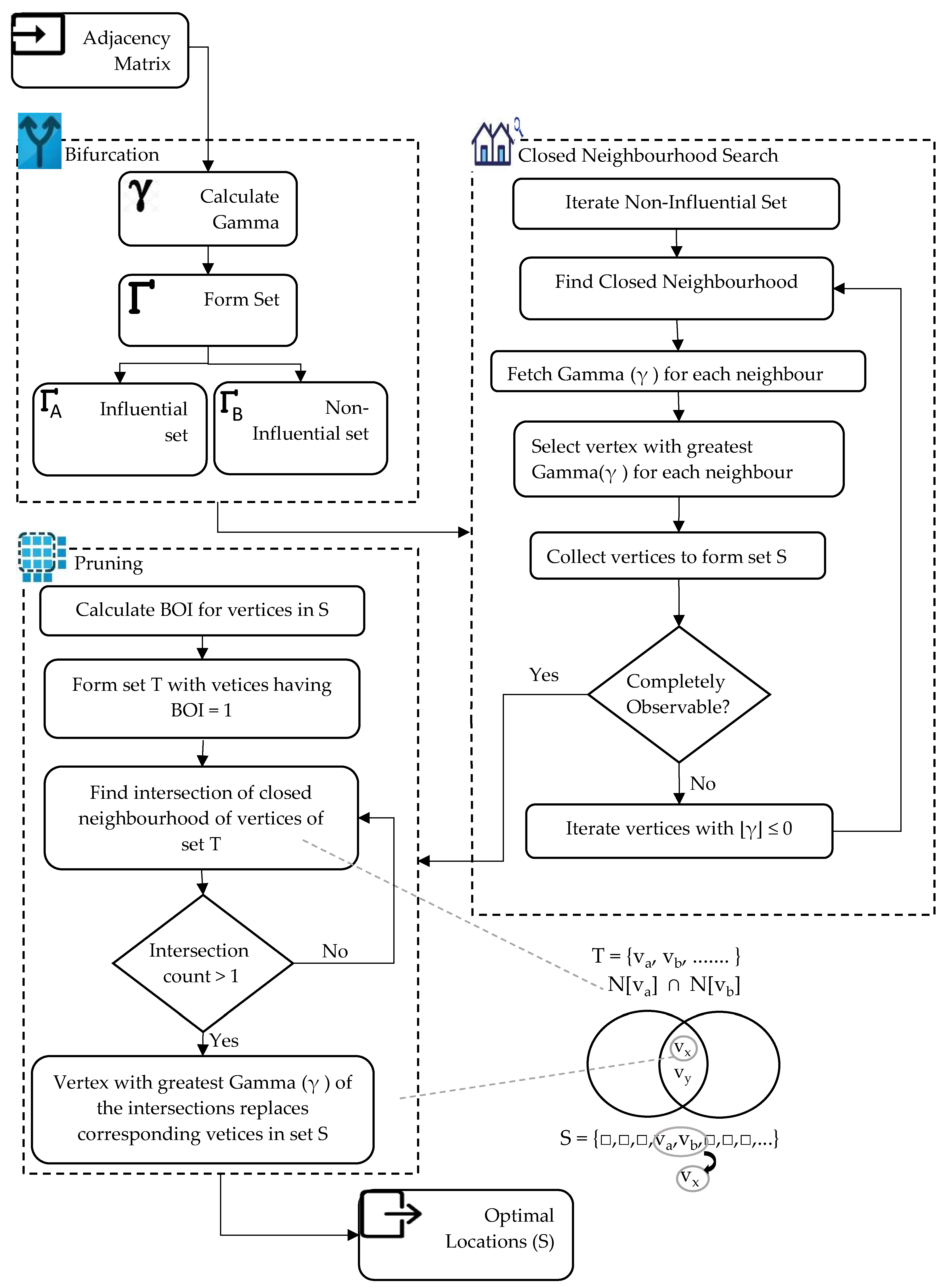
4. Solution Methodology

The defined OPP problem is solved based on the values of $\gamma$. The proposed method is divided into three stages.

4.1. Bifurcation

Vertices are arranged based on $\gamma$ and a new set, $\mathsf{\Gamma }$, is formed. The set $\mathsf{\Gamma }$ is obtained by arranging the vertices with $\gamma$ in decreasing order. That is,

$$\mathsf{\Gamma }=\{v_i,v_j,\dots /\gamma \left(v_i\right)\ge \gamma \left(v_j\right)\forall v_i,v_j\in V\left(G\right)\}$$

(14)

This set is then divided into two sets, namely the influential and non-influential sets. Therefore,

$$\mathsf{\Gamma }=\{{\mathsf{\Gamma }}_A\cup {\mathsf{\Gamma }}_B\}\mathrm{and}{\mathsf{\Gamma }}_A\cap {\mathsf{\Gamma }}_B=\left\{\right\}$$

(15)

where the first $⌊\frac{N}{2}⌋$ vertices in $\mathsf{\Gamma }$ form the influential set ${\mathsf{\Gamma }}_A$ and the remaining vertices in $\mathsf{\Gamma }$ form the non-influential set ${\mathsf{\Gamma }}_B$.

The vertices of the influential set are a degree greater than or equal to the average degree of their neighbouring vertices, whereas the vertices of the non-influential set have one or more neighbours with a greater degree. The process at this stage is presented in Algorithm 1 and is also discussed considering an IEEE seven-bus system.

Algorithm 1 Bifurcation $(n,D,A_m)$

for i in V do   sum_neighbour_degree $=0$   for neighbour_vertex in $A_m\left(i\right)$ do    sum_neighbour_degree = sum_neighbour_degree +D(neighbour_vertex)   end for   $\left(i\right)=D\left(i\right)-$(sum_neighbour_degree/$D\left(i\right)$)   $\mathsf{\Gamma }$[i][0] = i   $\mathsf{\Gamma }$[i][1] = (i)  end for  $\mathsf{\Gamma }=$ sort($\mathsf{\Gamma }$, descending)    //splitting $\mathsf{\Gamma }$ Array into Influential Vertices and Non-  Influential Vertices  $nA=$ ceil($n/2$)  $nB=n-nA$  $A=$ Ascending ($\mathsf{\Gamma }$[1 to $nA$])  $B=$ Ascending ($\mathsf{\Gamma }$[$nA+1$ to n])

For an IEEE seven-bus system, the sets $\mathsf{\Gamma }$, ${\mathsf{\Gamma }}_A$ and ${\mathsf{\Gamma }}_B$ are

$$\mathsf{\Gamma }=\{v_2,v_4,v_3,v_5,v_7,v_6,v_1\}$$

(16)

$${\mathsf{\Gamma }}_A=\{v_2,v_4,v_3\}\mathrm{and}{\mathsf{\Gamma }}_B=\{v_5,v_7,v_6,v_1\}$$

(17)

The vertices in the influential set correspond to greater values of $\gamma$ and are prone to be selected as an optimal location. This is because these vertices with higher degrees observe a good number of vertices but may not ensure complete observability. Since the vertices in the non-influential set are devoid of PMUs, to observe these vertices, a PMU must be placed in their neighbourhood. Hence, a closed neighbourhood search in the entities of the non-influential set is deployed at the next stage.

4.2. Closed Neighbourhood Search (CNS)

In this stage, the closed neighbourhoods of the vertices of the non-influential set are analyzed. Among the vertices in the closed neighbourhood, the vertex $v_i$ with the greatest $\gamma$ value is chosen as an optimal location. Let S represent the set containing the selected vertices at this stage. Initially, $S:$$=\left\{\right\}$ and $N\left[S\right]:$$=\left\{\right\}$.

The set S is updated as $S:$$=S\cup \left\{v_i\right\}$ at every iteration if $N\left[v_i\right]\cap N\left[S\right]\ne N\left[v_i\right]$. The iterations proceed by analyzing the closed neighbourhood of all vertices in the non-influential set until complete observability is reached. Observability is verified at the end of every iteration using the relation $N\left[S\right]=V\left(G\right)$. When the observability condition is satisfied, the vertices in S at that iteration may form the optimal solution set.

In case observability is not reached even after exhaustively searching the closed neighbourhood of the vertices in ${\mathsf{\Gamma }}_B$, a similar search is extended to the vertices in ${\mathsf{\Gamma }}_A$ whose $⌊\gamma ⌋\le 0$. This occurs especially in higher-order bus systems. Thus, a near optimal solution is obtained at this stage. The steps involved in this stage for an IEEE seven-bus system are explained in

Table 2. Process flow of closed neighbourhood search for IEEE seven-bus system.

Iteration $\left(\mathit{k}\right)$	${\mathsf{\Gamma }}_{\mathit{B}}\left(\mathit{k}\right)$	$\mathit{N}\left[{\mathsf{\Gamma }}_{\mathit{B}}\left(\mathit{k}\right)\right]$	${\mathit{v}}_{\mathit{i}}$	$\mathit{N}\left[{\mathit{v}}_{\mathit{i}}\right]$	S	$\mathit{N}\left[\mathit{S}\right]$
1	$v_5$	$\{v_4,v_5,v_7\}$	$v_4$	$\{v_3,v_4,v_5,v_7\}$	$\left\{v_4\right\}$	$\{v_3,v_4,v_5,v_7\}$
		$\gamma \left(v_4\right)>\gamma \left(v_5\right)$
		$\gamma \left(v_4\right)>\gamma \left(v_7\right)$
2	$v_7$	$\{v_4,v_5,v_7\}$	$v_4$	$\{v_3,v_4,v_5,v_7\}$	$\left\{v_4\right\}$	$\{v_3,v_4,v_5,v_7\}$
		$\gamma \left(v_4\right)>\gamma \left(v_5\right)$
		$\gamma \left(v_4\right)>\gamma \left(v_7\right)$
3	$v_6$	$\{v_2,v_3,v_6\}$	$v_2$	$\{v_1,v_2,v_3,v_6\}$	$\{v_2,v_4\}$	$\{v_1,v_2,v_3,v_4,v_5,v_6,v_7\}$
		$\gamma \left(v_2\right)>\gamma \left(v_3\right)>\gamma \left(v_6\right)$

. The iteration stops if $N\left[S\right]=V\left(G\right)$. Algorithm 2 explains the steps followed in this approach.

Algorithm 2 Closed Neighbourhood Search $(\mathsf{\Gamma },A,B,n)$

S = set()                // Optimal Solution Set  $k=1$                // Counter  for bRow in B do   while $\left(N\right[S]\ne V[G\left]\right)$ do    nodes $=b$Row$\left[0\right]$∪$A_m$(bRow$\left[0\right]$) // closed neighbourhood    $s_k=$ MAX ($\mathsf{\Gamma }$[nodes])    $N\left[s_k\right]=s_k\cup A_m\left(s_k\right)$    if $(N\left[s_k\right]\cap N\left[S\right]\ne N\left[s_k\right])$ then     S.add$\left(s_k\right)$;     $k=k+1$    end if   end while  end for  if (length $\left(N\right[S\left]\right)<n$) then   for aRow in A do    while $\left(N\right[S]\ne V[G\left]\right)$ do     nodes $=a$Row$\left[0\right]$∪$A_m$(aRow$\left[0\right]$)     $s_k=$ MAX($\mathsf{\Gamma }$[nodes])     $N\left[s_k\right]=s_k\cup A_m\left(s_k\right)$     if $(N\left[s_k\right]\cap N\left[S\right]\ne N\left[s_k\right])$ then      S.add($s_k$);      $k=k+1$     end if    end while   end for  end if

4.3. Pruning

This is the final verification stage to further reduce the set S.

In the second stage, the CNS might lead to the local minimum solution set. To avoid this, pruning is used. Hurtgen et al. suggest making a random move in the neighbourhood to avoid local minima [17]. This stage defines certain rules to further optimize the results obtained in the previous stage and is more appropriate to higher-order systems. This reduces the placement locations by investigating the BOI and the closed neighbourhood of every element in S.

The BOI for a bus (i) is the count that defines the number of times that bus is observed either directly or indirectly by a PMU. The SORI of a system is the sum of the BOI of all buses in the network. The factors of the BOI and SORI are used to evaluate the quality of optimal placement locations [5,13].

The steps involved in Algorithm 3 are explained as follows:

• The observability of every vertex is scrutinized and the BOI is calculated for every vertex;
• The vertices belonging to the set S with BOI equal to one are considered. Let T be the set of vertices belonging to S with a BOI equal to one. The set $T=\{v_a,v_b,\cdots \}$ is defined as the temporary set of vertices that has to be processed at this stage;
• An intersection of the closed neighbourhood of every vertex $v_a$ in set T and the closed neighbourhood of every other vertex $v_b$ in T is taken. If the result of this intersection is only two vertices—say, $\{v_x,v_y\}$—then it could be inferred that any one of these vertices $\{v_x,v_y\}$ could be used to observe the vertices $v_a$ and $v_b$. Among $v_x$ and $v_y$, the vertex that corresponds to the highest $\gamma$ replaces the original locations $v_a$ and $v_b$ in set S.

Thus, the redundant PMUs are cropped, and the solution reaches a global optimum.

Algorithm 3 Pruning $(V,S,A_m)$

placementMap = Map()  for s in S do   $N\left[s\right]=A_m\left(s\right)\cup s$   difference $=N\left[s\right]\cap N[S-s]$   singleNode = difference$\left[0\right]$   if (length(difference) $==1$ && singleNode $\ne s$) then    placementMap.append($s:$singleNode $\cup A_m$(singleNode))   end if  end for  $X=S$  for p in placementMap do   for j in placementMap do    if $(p\ne j)$ then     $I=$ (p∪ placementMap(p)) ∩ (j∪ placementMap(j))     if (len$\left(I\right)>0$) then      X.remove(p)      X.remove(j)      X.append($I\left[0\right]$)     end if    end if   end for  end for

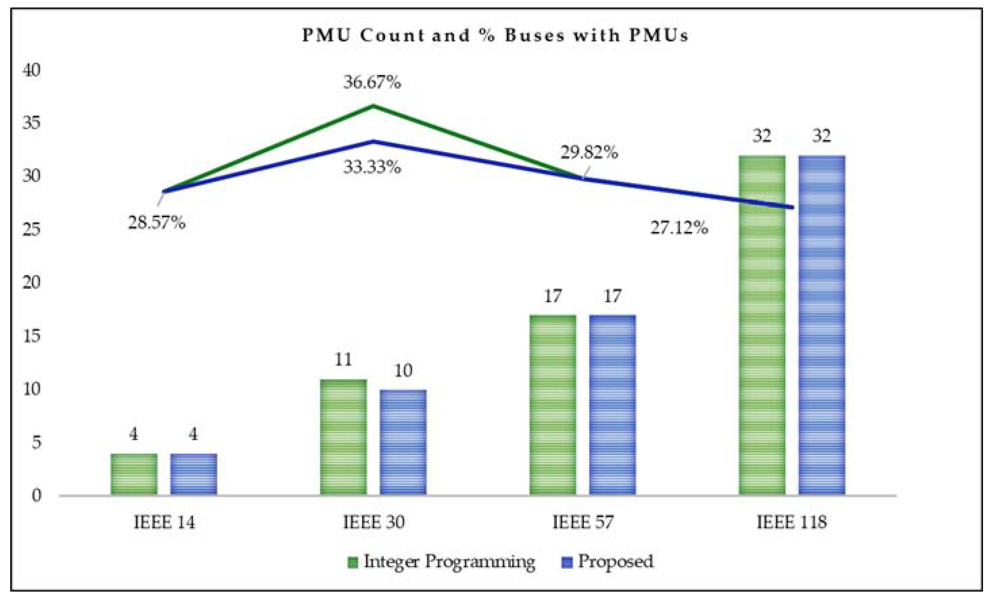
5. Simulation Results

The algorithm was tested for standard IEEE test systems including a hybrid AC/DC microgrid system. This microgrid system [40] consisted of both AC and DC generation sources supplying a hybrid set of loads that operated with both AC and DC power.

The results obtained in all three stages for the proposed methodology are shown in

Table 3. Stage-wise results for the proposed methodology.

System	Stage 1	Stage 2	Stage 3
IEEE 14	2, 6, 7, 9	2, 6, 7, 9	2, 6, 7, 9
IEEE 30	2, 4, 6, 9, 10, 12, 15, 19, 25, 27	2, 4, 6, 9, 10, 12, 15, 19, 25, 27	2, 4, 6, 9, 10, 12, 15, 19, 25, 27
IEEE 57	1, 4, 6, 9, 15, 20, 24, 27, 29, 30, 32, 36, 37, 38, 41, 46, 51, 53, 56	32, 1, 36, 37, 4, 38, 41, 9, 46, 15, 51, 20, 53, 24, 56, 27, 29, 30	1, 4, 9, 15, 20, 24, 27, 29, 30, 32, 36, 38, 41, 46, 51, 53, 57
IEEE 118	1, 5, 9, 12, 15, 17, 19, 21, 23, 27, 29, 30, 32, 34, 37, 40, 44, 46, 49, 52, 56, 59, 62, 65, 68, 70, 71, 75, 77, 80, 85, 86, 89, 92, 96, 100, 105, 110	1, 5, 9, 12, 15, 17, 21, 27, 29, 30, 32, 34, 37, 40, 44, 46, 49, 52, 56, 59, 62, 65, 68, 70, 71, 75, 77, 80, 85, 86, 89, 92, 96, 100, 105, 110	1, 5, 9, 12, 15, 17, 20, 23, 28, 30, 36, 40, 44, 46, 49, 52, 56, 62, 63, 68, 71, 75,77, 80, 85, 86, 90, 94, 102, 105, 110, 115
Hybrid AC/DC microgrid	2, 6, 7, 11, 14	2, 6, 7, 11, 14	2, 6, 7, 11, 14

. It could be seen that in the case of lower-order systems, an optimal solution was reached in stage 2, and a further reduction in stage 3 occurred only for higher-order systems.

The parameters of the BOI and SORI act as a measure of redundancy. The number of measurements obtained from a vertex increases as a greater number of lines are connected to that vertex. This tendency is represented as the Bus Observability Index (BOI).

The concept of the BOI ensures an evenly dispersed distribution of PMUs around the network, thereby limiting the number of PMUs, whereas the SORI is an indication of measurement redundancy.

Table 4. Comparison of the effectiveness of the proposed method with the integer programming method.

Method	Integer Programming Method		Proposed Method
System	Optimal PMU Locations	SORI	Optimal PMU Locations	BOI	SORI
IEEE 14	2, 8, 10, 13	14	2, 6, 7, 9	1,1,1,3,2,1,2,1,2,1,1,1,1,1	19
IEEE 30	1, 7, 8, 10, 11, 12, 19, 23, 26, 30, 34	34	2, 4, 6, 9, 10, 12, 15, 19, 25, 27	1,3,1,4,1,5,1,1,3,3,1,2,1,2,1,1, 1,2,1,2,1,1,1,1,2,1,2,2,1,1	50
IEEE 57	2, 6, 12, 15, 19, 22, 25, 27, 32, 36, 38, 41, 46, 50, 52, 55, 57	67	1, 4, 9, 15, 20, 24, 27, 29, 30, 32, 36, 38, 41, 46, 51, 53, 57	2,1,2,1,1,1,1,1,1,2,2,1,2,2,2,1,1,1,1, 1,1,1,1,1,2,2,1,2,1,1,2,1,1,1,1,1,2,1, 1,1,1,1,1,1,1,1,1,1,1,1,1,2,1,1,1,2,1	71
IEEE 118	2, 5, 10, 12, 15, 17, 21, 25, 29, 34, 37, 41, 45, 49, 53, 56, 62, 64, 72, 73, 75, 77, 80, 85, 87, 91, 94, 101, 105, 110, 114, 116	149	1, 5, 9, 12, 15, 17, 20, 23, 28, 30, 36, 40, 44, 46, 49, 52, 56, 62, 63, 68, 71, 75, 77, 80, 85, 86, 90, 94, 102, 105, 110, 115	1,2,3,1,1,1,1,3,1,1,2,1,1,2,2,2,3,1, 2,1,1,1,1,1,1,1,2,1,1,2,1,1,1,1,1,1, 1,1,1,1,1,2,1,1,3,1,2,2,1,1,2,1,1,2, 1,1,2,1,2,1,1,1,1,1,1,2,1,1,4,2,1,1, 1,1,2,1,2,1,1,2,2,1,1,1,2,2,1,1,2,1, 1,1,2,1,1,2,1,1,1,1,1,1,2,1,1,1,1,1, 1,1,1,1,1,1,1,1,1,1	156
Hybrid AC/DC microgrid	NA	NA	2, 6, 7, 11, 14	1,1,1,2,2,2,1,1, 2,1,2,1,2,1,1	21

shows a comparison of the OPP based on integer programming methods [13] and the proposed method.

The number of PMUs required for complete observability is the same for all the systems. However, the BOI and SORI depend on the choice of optimal placement locations. If a PMU is placed at a radial bus, it makes two buses observable, but if a PMU is placed at a bus to which a radial bus is connected, it makes more than two buses observable [41]. In the proposed method, this is achieved by prioritizing the node with the maximum degree. Thus, the SORI is improved. The proposed method was executed using Algorithm 4. Figure 2 presents the framework of proposed methodology.

Algorithm 4 Find Optimal Placement$\left(A\right)$

//A—Adjacency Matrix  //n—Number of vertices  //D—Degree Vector of each vertex  //V—Set of Vertices  //$A_m$—Adjacency Map—i.e., $\{v_1:(v_2,v_4),v_2:(v_1,v_5,v_6),\dots v_n\}$  $[\mathsf{\Gamma },A,B]=$ bifurcation$(D,A_m)$   //$\mathsf{\Gamma }$—Gamma Array i.e., $[(v_1,1),(v_2,2),\dots ,(v_n,n)]$  $S=$ ClosedNeighbourhoodSearch$(\mathsf{\Gamma },A,B,n)$  $X=$ pruning$(V,S,A_m)$

A comparison of the PMU count and percentage of buses for different IEEE standard systems allocated with PMUs by integer programming and the proposed method are shown in Figure 3. Figure 3 shows that the number of PMUs recommended by the proposed method is either equal to or less than the count suggested by the integer programming method. Figure 4 depicts the improvement in the SORI with the proposed method compared to integer programming.

With greater values of the SORI for the proposed method, it is evident that the proposed method would render a greater measurement redundancy. Thus, it can be concluded that the solution obtained is a global optimal solution.

The algorithm was programmed and implemented using Python. NumPy is a Python library used for programming. This program was implemented on a Core i7, 2.4 GHz PC with 8.00 GB RAM.

The computation time for the considered test systems in milliseconds is given in

Table 5. Stage-wise computation time in milliseconds of the algorithm for various test systems.

System	Stage 1	Stage 2	Stage 3	Total
IEEE 14	6.7	1.13	0.1	7.93
IEEE 30	10	1.9	0.2	12.1
IEEE 57	11.2	3.4	0.4	15
IEEE 118	19	7.5	2	28.5
Hybrid AC/DC microgrid	7.5	1.5	0.1	9.1

.

It is evident from Table 5 that the proposed algorithm took only a few milliseconds and thus was proven to be fast.

6. Conclusions

The proposed method identifies and highlights the property of three major attributes in deciding placement locations: the degree of the vertex, the average neighbourhood degree of the vertex, and the BOI.

• The degree of the vertex helps to maximize the measurement redundancy;
• The average neighbourhood degree and the BOI aid in reaching a global optimal solution.

A unique attempt to interlace these attributes has been made and was proven to be successful. A three-stage algorithm has been proposed in which the first two stages ensure the maximization of the measurement redundancy and the third stage confirms the selection of minimum number of PMUs. Minimizing the number of PMUs reduces the investment cost on PMUs required to completely observe the system. The main concern for optimally placing PMUs is to improve the state estimation process. For this, the system has to be completely observable, and also a good measurement redundancy has to be maintained. It can be seen from the values of the BOI and SORI that system was completely observed and also measurement redundancy was improved in our experiment. The following are evident from the results:

• The number of PMUs computed for a system to be completely observable is minimum;
• The chosen strategic locations improve the measurement redundancy;
• The improved redundant data aid in obtaining more reliable estimates through state estimation;
• The complexity of the proposed algorithm is $O\left(n\right)$, and hence it is simple, fast and easy to implement;
• The proposed technique is generalized and could be extended to systems of higher order and even to microgrid systems.

A majority of the earlier contributions concentrate only on reducing the investment cost. Like other contributions, the proposed method reduces the PMU count, maintaining complete observability; in addition, it also improves measurement redundancy.

References

1. IEEE Standards Association. IEEE Guide for Synchronization, Calibration, Testing, and Installation of Phasor Measurement Units (PMUs) for Power System Protection and Control IEEE Power and ENERGY Society; IEEE Standard C; IEEE Standards Association: Piscataway, NJ, USA, 2013; pp. 1–107. [Google Scholar]
2. Abur, A.; Exposito, A.G. Power System State Estimation: Theory and Implementation; Mercel Dekker: New York, NY, USA, 2004. [Google Scholar]
3. Zhao, H.-S.; Ying, L.; Mi, Z.-Q.; Lei, Y. Sensitivity Constrained PMU Placement for Complete Observability of Power Systems. In Proceedings of the 2005 IEEE/PES Transmission & Distribution Conference & Exposition: Asia and Pacific, Dalian, China, 15–18 August 2005; pp. 1–5. [Google Scholar] [CrossRef]
4. Zhang, P. Phasor Measurement Unit (PMU) Implementation and Applications; Electric Power Research Institute: Palo Alto, CA, USA, 2007. [Google Scholar]
5. Dua, D.; Dambhare, S.; Gajbhiye, R.K.; Soman, S.A. Optimal Multistage Scheduling of PMU Placement: An ILP Approach. IEEE Trans. Power Deliv. 2008, 23, 1812–1820. [Google Scholar] [CrossRef]
6. Gomathi, V.; Ramachandran, V. Optimal location of PMUs for complete observability of power system network. In Proceedings of the 1st International Conference on Electrical Energy Systems, Chennai, India, 3–5 January 2011; pp. 314–317. [Google Scholar] [CrossRef]
7. Azizi, S.; Dobakhshari, A.S.; Sarmadi, S.A.N.; Ranjbar, A.M. Optimal PMU Placement by an Equivalent Linear Formulation for Exhaustive Search. IEEE Trans. Smart Grid 2012, 3, 174–182. [Google Scholar] [CrossRef]
8. Mahaei, S.M.; Hagh, M.T. Minimizing the number of PMUs and their optimal placement in power systems. Electric Power Syst. Res. 2012, 83, 66–72. [Google Scholar] [CrossRef]
9. Huang, L.; Sun, Y.; Xu, J.; Gao, W.; Zhang, J.; Wu, Z. Optimal PMU Placement Considering Controlled Islanding of Power System. IEEE Trans. Power Syst. 2014, 29, 742–755. [Google Scholar] [CrossRef]
10. Bhonsle, J.; Junghare, A. Optimal placing of PMUs in a constrained grid: An approach. Turk. J. Electr. Eng. Comput. Sci. 2016, 24, 4508–4516. [Google Scholar] [CrossRef]
11. Aghaei, J.; Baharvandi, A.; Rabiee, A.; Akbari, M. Probabilistic PMU Placement in Electric Power Networks: An MILP-Based Multiobjective Model. IEEE Trans. Ind. Inform. 2015, 11, 332–341. [Google Scholar] [CrossRef]
12. Chen, X.; Sun, L.; Chen, T.; Sun, Y.; Rusli Tseng, K.J.; Ling, K.V.; Ho, W.K.; Amaratunga, G.A.J. Full Coverage of Optimal Phasor Measurement Unit Placement Solutions in Distribution Systems Using Integer Linear Programming. Energies 2019, 12, 1552. [Google Scholar] [CrossRef] [Green Version]
13. Rahman, N.H.A.; Zobaa, A.F. Optimal PMU placement using topology transformation method in power systems. J. Adv. Res. 2016, 7, 625–634. [Google Scholar] [CrossRef] [Green Version]
14. Anas, A.; Lingling, F. Optimal PMU placement for modeling power grid observability with mathematical programming methods. Int. Trans. Electr. Energy Syst. 2019, 30, e12182. [Google Scholar] [CrossRef]
15. Bečejac, V.; Stefanov, P. Groebner bases algorithm for optimal PMU placement. Int. J. Electr. Power Energy Syst. 2020, 115, 105427. [Google Scholar] [CrossRef]
16. Chakrabarti, S.; Kyriakides, E. Optimal Placement of Phasor Measurement Units for Power System Observability. IEEE Trans. Power Syst. 2008, 23, 1433–1440. [Google Scholar] [CrossRef]
17. Hurtgen, M.; Maun, J.C. Optimal PMU placement using Iterated Local Search. Int. J. Electr. Power Energy Syst. 2010, 32, 857–860. [Google Scholar] [CrossRef]
18. Ahmadi, A.; Alinejad-Beromi, Y.; Moradi, M. Optimal PMU placement for power system observability using binary particle swarm optimization and considering measurement redundancy. Expert Syst. Appl. 2011, 38, 7263–7269. [Google Scholar] [CrossRef]
19. Hajian, M.; Ranjbar, A.M.; Amraee, T.; Mozafari, B. Optimal placement of PMUs to maintain network observability using a modified BPSO algorithm. Int. J. Electr. Power Energy Syst. 2011, 33, 28–34. [Google Scholar] [CrossRef]
20. Koutsoukis, N.C.; Manousakis, N.M.; Georgilakis, P.S.; Korres, G.N. Numerical observability method for optimal phasor measurement units placement using recursive Tabu search method. IET Gener. Transm. Distrib. 2013, 7, 347–356. [Google Scholar] [CrossRef]
21. El-Zonkoly, A.; El-Safty, S.; Maher, R. Optimal placement of PMUs using improved tabu search for complete observability and out-of-step prediction. Turk. J. Electr. Eng. Comput. Sci. 2013, 21, 1376–1393. [Google Scholar] [CrossRef] [Green Version]
22. Singh, S.P. Optimal placement of phasor measurement units using gravitational search method. Int. J. Electr. Comput. Electron. Commun. Eng. 2015, 9, 274–278. [Google Scholar] [CrossRef]
23. Dalali, M.; Karegar, H.K. Optimal PMU placement for full observability of the power network with maximum redundancy using modified binary cuckoo optimization algorithm. IET Gener. Transm. Distrib. 2016, 10, 2817–2824. [Google Scholar] [CrossRef]
24. Müller, H.H.; Castro, C.A. Genetic algorithm-based phasor measurement unit placement method considering observability and security criteria. IET Gener. Transm. Distrib. 2016, 10, 270–280. [Google Scholar] [CrossRef]
25. Maji, T.K.; Acharjee, P. Multiple Solutions of Optimal PMU Placement Using Exponential Binary PSO Algorithm for Smart Grid Applications. IEEE Trans. Ind. Appl. 2017, 53, 2550–2559. [Google Scholar] [CrossRef]
26. Saleh, A.; Adail, A.S.; Wadoud, A.A. Optimal phasor measurement units placement for full observability of power system using improved particle swarm optimization. IET Gener. Transm. Distrib. 2017, 11, 1794–1800. [Google Scholar] [CrossRef]
27. Bashian, A.; Assili, M.; Anvari-Moghaddam, A. A security-based observability method for optimal PMU-sensor placement in WAMS. Int. J. Electr. Power Energy Syst. 2020, 121, 106157. [Google Scholar] [CrossRef]
28. Abdelsalam, A.A.; Hassanin, K.M.; Abdelaziz, A.Y.; Alhelou, H.H. Optimal PMUs placement considering ZIBs and single line and PMUs outages. AIMS Energy 2020, 8, 122–141. [Google Scholar] [CrossRef]
29. Baldwin, T.L.; Mili, L.; Boisen, M.B.; Adapa, R. Power system observability with minimal phasor measurement placement. IEEE Trans. Power Syst. 1993, 8, 707–715. [Google Scholar] [CrossRef]
30. Denegri, G.B.; Invernizzi, M.; Milano, F. A security oriented approach to PMU positioning for advanced monitoring of a transmission grid. In Proceedings of the International Conference on Power System Technology, Kunming, China, 13–17 October 2002; Volume 2, pp. 798–803. [Google Scholar] [CrossRef]
31. Haynes, T.W.; Hedetniemi, S.M.; Hedetniemi, S.T.; Henning, M.A. Domination in Graphs Applied to Electric Power Networks. SIAM J. Discret. Math. 2002, 15, 519–529. [Google Scholar] [CrossRef]
32. Nuqui, R.F.; Phadke, A.G. Phasor measurement unit placement techniques for complete and incomplete observability. IEEE Trans. Power Deliv. 2005, 20, 2381–2388. [Google Scholar] [CrossRef]
33. Venugopal, G.; Velayutham, U. Optimal placement of PMU based on vertex colouring and AVL tree technique. Int. J. Appl. Eng. Res. 2015, 10, 13841–13853. [Google Scholar]
34. Devi, M.M.; Geethanjali, M. Hybrid of Genetic Algorithm and Minimum Spanning Tree method for optimal PMU placements. Measurement 2020, 154, 107476. [Google Scholar] [CrossRef]
35. Kong, X.; Wang, Y.; Yuan, X.; Yu, L. Multi Objective for PMU Placement in Compressed Distribution Network Considering Cost and Accuracy of State Estimation. Appl. Sci. 2019, 9, 1515. [Google Scholar] [CrossRef] [Green Version]
36. Srinivas, N.; Deb, K. Multi-objective function optimization using nondominated sorting genetic algorithms. Evol. Comput. 1994, 2, 221–248. [Google Scholar] [CrossRef]
37. Peng, C.; Sun, H.; Guo, J. Multi-objective optimal PMU placement using a non-dominated sorting differential evolution algorithm. Int. J. Electr. Power Energy Syst. 2010, 32, 886–892. [Google Scholar] [CrossRef]
38. Saravanan, M.; Sujatha, R.; Sundareswaran, R.; Balasubramanian, M. Application of domination integrity of graphs in PMU placement in electric power networks. Turk. J. Electr. Eng. Comput. Sci. 2018, 26, 2066–2076. [Google Scholar] [CrossRef]
39. Deo, N. Graph Theory with Applications to Engineering and Computer Science; Prentice Hall Inc.: New Delhi, India, 1974. [Google Scholar]
40. Ortiz, L.; Orizondo, R.; Águila, A.; González, J.W.; López, G.J.; Isaac, I. Hybrid AC/DC microgrid test system simulation: Grid-connected mode. Heliyon 2019, 5, e02862. [Google Scholar] [CrossRef] [PubMed] [Green Version]
41. Roy, B.K.S.; Sinha, A.K.; Pradhan, A.K. An optimal PMU placement technique for power system observability. Int. J. Electr. Power Energy Syst. 2012, 42, 71–77. [Google Scholar] [CrossRef]
Short Biography of Authors
Lourdusamy Ramya Hyacinth completed her bachelor’s degree in Electrical and Electronics Engineering from Government College of Engineering, Tirunelveli, Tamilnadu, India in 2011. Later completed Master of Engineering in the field of Power Systems at College of Engineering, Guindy, Anna University, Chennai, Tamilnadu, India in 2013. She is at present an Assistant Professor at Loyola-ICAM College of Engineering and Technology, Nungambakkam, Chennai, Tamilnadu, India. Also, she is currently pursuing her research at Anna University, Chennai, India. Her field of interests include Power System State Estimation, Optimal PMU Placement, Bad Data Analysis and IoT based services for power systems.
Venugopal Gomathi completed her bachelor’s degree in Electrical and Electronics Engineering from Madras University, Chennai, Tamilnadu, India in 2002. Later, completed Master of Engineering in 2004 and Ph.D in 2011 in the field of Power Systems at College of Engineering, Guindy, Anna University, Chennai, Tamilnadu, India. She is an Associate Professor in the Department of Electrical and Electronics Engineering at College of Engineering Guindy, Anna University, Chennai, Tamilnadu, India. Her research interests include Power System operation and Control, State estimation, Modelling and Control of Smart Grids and Microgrids, Congestion Management, Distributed Demand response and Cloud Services for Power system control.
Figure 1. Plot of γ for IEEE seven-bus system.
Energies 14 04782 g001
Figure 2. Framework of the proposed method.
Energies 14 04782 g002
Figure 3. Variation of bus count and percentage of buses allocated with PMUs.
Energies 14 04782 g003
Figure 4. SORI of integer programming vs. proposed method.
Energies 14 04782 g004