Abstract
Photovoltaic (PV) power forecasting urges in economic and secure operations of power systems. To avoid an inaccurate individual forecasting model, we propose an approach for a one-day to three-day ahead PV power hourly forecasting based on the stacking ensemble model with a recurrent neural network (RNN) as a meta-learner. The proposed approach is built by using real weather data and forecasted weather data in the training and testing stages, respectively. To accommodate uncertain weather, a daily clustering method based on statistical features, e.g., daily average, maximum, and standard deviation of PV power is applied in the data sets. Historical PV power output and weather data are used to train and test the model. The single learner considered in this research are artificial neural network, deep neural network, support vector regressions, long short-term memory, and convolutional neural network. Then, RNN is used to combine the forecasting results of each single learner. It is also important to observe the best combination of the single learners in this paper. Furthermore, to compare the performance of the proposed method, a random forest ensemble instead of RNN is used as a benchmark for comparison. Mean relative error (MRE) and mean absolute error (MAE) are used as criteria to validate the accuracy of different forecasting models. The MRE of the proposed RNN ensemble learner model is 4.29%, which has significant improvements by about 7–40%, 7–30%, and 8% compared to the single models, the combinations of fewer single learners, and the benchmark method, respectively. The results show that the proposed method is promising for use in real PV power forecasting systems.
1. Introduction
Photovoltaic (PV) power generation forecasting has become one of the most important aspects of renewable energy integration to the smart grid. PV power integration to a low-voltage weak grid system is beneficial to strengthen the grid and improve the performance of the grid-integrated PV system [1,2,3]. However, as the PV power is vastly implemented, the harvested PV generation needs to be projected accurately. The difficulties in predicting the PV power comprise uncertain weather variables, such as temperature, wind speed, relative humidity, and irradiance, which are important for having a strong correlation to targeted PV power [4,5,6]. In addition, a forecasting algorithm is urgently required to build an optimal forecasting model that can predict the PV power accurately.
PV power forecasting has been researched by constructing a model that uses regression [7], a statistical method [8], a meta-heuristic method [9], and a hybrid method [10]. In Reference [7], Gaussian kernel support vector regression (SVR) is used as a forecasting model of PV energy due to the combination of numerical weather prediction and satellite data. However, this method provides the forecasting only for a short time horizon (6 h ahead). In Reference [8], an autoregressive moving average and exogenous input (ARMAX) model is used as the improvement of the autoregressive integrated moving average (ARIMA) model, which has limitations because the model cannot take the climate condition into considerations and results in notable error validation. Furthermore, pattern classification and particle swarm optimization [9] are used to optimize the weight of sky image cloud motion calculation to improve the accuracy of PV power forecasting. The drawback of this method is the high computational cost caused by the implementation of the optimization method compared to low prediction accuracy, which needs to be corrected. The hybrid metaheuristic and machine learning techniques for parameter optimization have been widely used in PV power forecasting, as reviewed in Reference [10].
Single forecasting algorithm in PV power generation is well-developed, such as in deep neural network (DNN) [11], convolutional neural network (CNN) [12], SVR [13], and random forest (RF) [14]. In Reference [11], the model is constructed using only historical PV power output data. Mean absolute error (MAE), root mean squared error (RMSE), and coefficient of determination (R2) are used as evaluation criteria. However, without including the meteorological variables, it is still difficult to obtain better accuracy for a longer time period.
Regarding the input variables, in Reference [12], the forecasting model is constructed using module temperature, solar radiance, and PV power output. MAE and RMSE are used as error validation. In Reference [13], the forecasting model is constructed using the same day of historical PV output power, the maximum, minimum, and average temperature. Mean relative error (MRE) and RMSE are used to evaluate accuracy. The results show that the MRE is still relatively high, especially for cloudy, foggy, and rainy days. In Reference [14], the forecasting model is constructed using temperature, atmospheric pressure, relative humidity, wind speed, PM2.5 air pollution concentration, and total solar radiation. MAE, mean absolute percentage error (MAPE), RMSE, and explained variance (EV) are used as performance evaluation indicators. The results show that the accuracy on rainy or snowy days is higher than on clear and cloudy days.
In addition, probabilistic PV power forecasting has also been developed. A high-order Markov chain is implemented to model the generated PV power and used to forecast the probability distribution function (PDF) of PV power [15] by using historical PV output power, ambient temperature, and solar irradiance as input. Continuous rank probability score (CRPS) is used to observe the performance of forecasting PDF, while MAE is used to measure the error of point forecasting. In Reference [16], the prediction model is constructed by an improved Markov chain, having historical PV power, radiation, wind speed, temperature, humidity, and wind direction as input variables. MAE, RMSE, and quantile score are used as evaluation criteria, and the width of the forecasting interval is calculated.
In Reference [17], a forecasting model is constructed using ensemble learning of the linear method, the normal distribution method, and the normal distribution method with additional features. Twelve environmental variables are used as input to the model, and RMSE and MAE are used as evaluation metrics for point forecasting, while the pinball-loss function is used for probabilistic forecasting. Even though the probabilistic PV power is promising, it is difficult for the system operators to understand the result with no prior experience.
Point forecasting is desirable since we need to further process the results of PV power forecasting to the subsequent processes, such as sending the power to the grid [18] or to the energy management system [19]. To improve forecasting accuracy, the ensemble method is preferable for use versus the single forecasting algorithm [20]. The ensemble method is the meta-learner forecasting algorithm [21]. In Raza et al. [22], the ensemble method builds from five FFNN structures, and each FFNN structure contains 20 different structures. Historical data for PV power output, solar irradiance, wind speed, temperature, and humidity are used as input. The performance indices used are MAPE and EV.
In Reference [23], an ensemble method is built based on the artificial neural network (ANN) models with different training data sets using the bagging technique. RMSE, MAE, and weighted mean absolute error are used as performance metrics. In addition, there are ensemble prediction intervals using the same ensemble model. The model uses prediction intervals coverage probability and prediction intervals width to validate this model. In Reference [24], the ensemble method builds from a group of decision trees to construct a random forest ensemble model. Normalized mean bias error (nMBE), normalized mean absolute error (nMAE), normalized RMSE (nRMSE), and skill score are used as evaluation metrics.
In this paper, we propose an accurate ensemble method combining five single models, which are ANN, DNN, SVR, long short-term memory (LSTM), and CNN, into a meta-learner algorithm for PV generation forecast of a real 200 kWp PV power plant in Taiwan. The meta-learner algorithm used in this paper is the recurrent neural network (RNN). ANN has a good capability for solving non-linear problems [25], while DNN is similar to ANN with two or more hidden layers. SVR performs lower computation, is easy to implement, and is robust to outliers [26]. LSTM has a memory to store long information and is good at handling sequence data [27,28]. CNN has a good capability to handle image input and can learn relevant features from an image. CNN also has a good performance in forecasting time series data by reshaping the data into 3D form as the input to CNN [29]. By incorporating these advantages, a stacking ensemble method with RNN as the meta-learner is formulated. RNN can capture the sequential information in the input data better than other models. In addition, RNN has parameter sharing, thus having fewer parameters to train and eases computational burden.
In this study, the ensemble of PV power forecasting with RNN as a meta-learner is compared to RF [30] as the benchmark model. To build the proposed ensemble forecasting method, the input variables are preprocessed through normalization and missing data correction, and then clustered into five weather types. Then, these data are fed to each single forecasting method. The result of each method is sent to the proposed RNN to obtain the final forecasting results. Our contributions can be highlighted as follows: (1) the implementation of RNN as a meta-learner in the stacking ensemble method is first used for PV power forecasting; (2) the proposed ensemble method is established based on the latest well-known single forecasting methods (i.e., ANN, DNN, SVR, LSTM, and CNN) before being fed to RNN as a meta-learner, and the combinations of the best three methods among them are observed; (3) the clustering method is implemented based on the daily average, maximum, and standard deviation of PV power output, a scheme that further improves the forecasting accuracy; and (4) real case studies are performed using data from a PV power plant in Taiwan with a nominal capacity of 200 kWp, with good contributions to the PV industry.
The remainder of this paper is organized as follows. The ensemble methods are reviewed in Section 2. Section 3 describes the proposed ensemble forecasting model. Section 4 describes the dataset and performance evaluation. The case study and discussion are described in Section 5. Finally, conclusions are discussed in Section 6.
2. Ensemble Methods
Ensemble techniques train multiple learners to increase forecasting accuracy. Unlike ordinary learning approaches that attempt to develop one learner, ensemble approaches aim to create a collection of learners from training data and merge them [31]. There are various techniques such as simple averaging [32], weighted averaging [32], bagging [33], boosting [34], and stacking [32] used to perform ensemble methods. Unlike algorithms for bagging and boosting, which originally combine single learners of the same type, the algorithm for stacking is typically applied to single learners constructed by various learning algorithms. Described below are the reviewed ensemble methods.
2.1. Simple Averaging
Simple averaging [32] is acquired by directly averaging the outputs of every single learner as follows:
where is the combined forecasting results, is a single learner’s forecasting results at the ith point, and N is the number of the single method.
2.2. Weighted Averaging
Weighted averaging [32] is acquired by averaging the outputs of single learners with dissimilar weights as follows:
where is the combined forecasting results, and is the weight for . is the single learner’s forecasting results at the ith point, and N is the number of the single method.
2.3. Bagging
Bagging (or bootstrap aggregating) [33] is the representation of the parallel ensemble technique. In this technique, the single learners are created in parallel. Bagging uses the bootstrap sampling technique to create multiple subsets (bags) of samples from the original dataset. The final prediction results are obtained by combining the prediction results from all subsets through averaging (1). Random forest is the most common algorithm used in the bagging technique.
2.4. Boosting
Boosting is a sequential ensemble process [34]. From the original dataset, several subsets are created. Each subsequent model tries to correct the errors of the previous model. A single method is created on this subset. The most inaccurate prediction will be assigned with a higher weight. Similar to the bagging technique, numerous models will be created to correct the errors from the previous model. Finally, the results will be obtained from the weighted average as used in (2). Algorithms used in the boosting technique are AdaBoost [35], gradient boosting machine (GBM) [36], extreme gradient boosting (XGBM) [37], and light gradient boosting machine (LGBM) [38].
2.5. Stacking
Stacking, also known as a stacked generalization, is an ensemble learning technique that runs the single learners (first-level learners) and combines them by training the meta-learner (second-level learner) to output prediction results [32]. Stacking uses the results of the predictions of multiple models to construct a new model. Generally, any learning algorithm can be used as a single learner and meta-learner. The stacking procedure is shown in Algorithm 1.
| Algorithm 1. Stacking procedure | |
| Input: | Dataset D = {(x1,y1),(x2,y2,…,(xm,ym)}; |
| First-level learning algorithm L1,…, LT; | |
| Second-level learning algorithm L. | |
| Process: | |
| 1. for t = 1,…,T: % Train a first-level learner by applying the | |
| 2. ht = Lt(D); % first-level learning algorithm Lt | |
| 3. end | |
| 4. D′ = Ø; % Generate a new dataset | |
| 5. for i = 1,…,m; | |
| 6. for t = 1,…,T: | |
| 7. Zit = | |
| 8. end | |
| 9. D′ = D′ ∪ ((zi1,…,ziT),yi); | |
| 10. end | |
| 11. h′ = L(D′); % Train the second-level learner h′ by applying | |
| % the second-level learning algorithm L to the | |
| % new dataset D′. | |
| Output: | |
3. The Proposed Ensemble PV Power Forecasting Algorithm
The proposed ensemble forecasting algorithm for PV power generation consists of the data preprocessing, five single algorithms, and meta-learner algorithm. Figure 1 shows the RNN-based ensemble method. The input of the single learner algorithms is the hourly historical PV power output and weather variables such as air temperature, relative humidity, and average wind speed with a duration of 12 h in one day from 06:00–17:00. n is the length of training or testing dataset of the single learner for each of the five weather types, for example, for sunny weather type, the training dataset (n) is 576 h (12 h × 48 days) in the training stage, and the testing dataset (n) is 156 h (12 h × 13 days) in the testing stage.
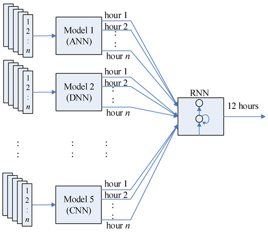
Figure 1.
Stacking procedure.
The forecasting results of single learners are fed to the RNN meta-learner as the training and testing dataset. In RNN, n is 144 h (12 h × 12 days) in the training stage and 12 h in the testing stage. As illustrated in Figure 1, the output results of every single learner model have one vector as the input to the ensemble learner. In our case, we have five single learner models, and the RNN input is a matrix of 5 by n. The output of the RNN meta-learner is the final ensemble forecasting results of 12 h for one-day ahead PV power forecasting.
To perform the three-day ahead PV power forecasting, the one-day ahead PV power forecasting is implemented and followed by the rolling-window technique as shown in Figure 2. For example, in step 1, we use the five-day training datasets as input to predict the next day’s PV power output Dt+1. In step 2, the five-day training datasets, including the prediction results obtained in step 1 (i.e., Dt+1), are employed as input to predict Dt+2. The third step employs the five-day training datasets, including the previous two-day predictions in steps 1 and 2, as input to predict Dt+3. The three-day ahead rolling window technique is performed per day to increase the accuracy of PV power forecasting. The forecasting horizon used in this study is 1–3 days ahead with hourly resolution.
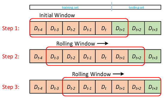
Figure 2.
The proposed RNN-based ensemble method.
In this paper, as an example, the capacity of the PV power plant in Taiwan for demonstration is 200 kWp. The data are taken from January to December 2019 with hourly observations. There are 20 days without weather prediction data, thus the total number of days is 345 days of data for constructing the proposed ensemble algorithm. We take only 12 h in one day where the PV power generation has output.
The training and testing stages are shown in Figure 3. Before preparing the training and testing data sets, the overall input data are classified into five different weather types using the fuzzy c-means (FCM) method based on the Calinski-Harabasz (CH) index. This treatment is performed to obtain better forecasting performance. Then, the classified weather data sets are sunny (61 days), light-cloudy (101 days), cloudy (96 days), heavy-cloudy (62 days), and rainy (25 days).
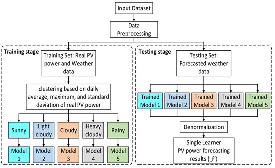
Figure 3.
A three-day ahead rolling window technique.
The detailed explanations regarding data preprocessing, single algorithms, and meta-learner are described as follows.
3.1. Data Preprocessing
There are three steps in data preprocessing to obtain good data as model input. First, the missing or broken data are replaced by new data from the cubic spline interpolation method. Second, the data are normalized between [0, 1] as follows:
where is the normalized data and is the original data with and as the maximum and minimum values of , respectively.
Third, the FCM method [39] is implemented to divide the data into five clusters according to different weather types. The optimal number of clusters is determined using Calinski-Harabasz (CH) index [40]. Then, the treated data are used to train every single model. FCM aims to minimize the objective function as follows:
where is the degree to which an observation belongs to a cluster . is the center of cluster , and is the fuzzifier. is a real number greater than one, and it defines the level of cluster fuzziness.
In fuzzy clustering, the centroid of a cluster is the mean of all points, and it is weighted by their degree of belonging to the cluster:
where is the centroid of cluster . Figure 4 shows five different weather types based on the clustering method.

Figure 4.
Flowchart for training and testing stages of each single model.
3.2. Single Forecasting Models
Every single forecasting model is used to extract the features of input variables. Models of ANN, DNN, SVR, LSTM, and CNN are used, and their characteristics, advantages, and disadvantages are summarized in Table 1. The ANN, DNN, SVR, LSTM, and CNN are briefly described as follows:

Table 1.
Summary of the single learner methods used.
3.2.1. Artificial Neural Network
The type of ANN is a feedforward neural network, which is a particular form of early artificial neural network known for its design simplicity. In ANN, there is an input layer, hidden layers, and output layer. The detailed network of ANN is referred to Reference [41].
3.2.2. Deep Neural Network
The type of DNN used in this study is the cascade-forward network with three hidden layers. The difference between the cascade-forward network and the ordinary feedforward network is the connection from the input layer and every previous layer to the following layers. A bias can also be added to the input layer, to which the detailed model refers to Reference [42]. The basic principle of the cascade-forward network is the same as the feedforward network.
3.2.3. Support Vector Regression
SVR is used to solve non-linear regression problems as follows:
where denotes the forecast values and is the kernel function (RBF function as a kernel function) of the inputs. and are adjustable coefficients that are weighted and biased, respectively. Through employing a penalty function to estimate the values of coefficients , the penalty function can be solved by a quadratic program as in Reference [43].
3.2.4. Long Short-Term Memory
LSTM [44] is the refined RNN that can memorize the pattern for long durations of time and can handle or learn the long-term dependencies. LSTM consists of cell state, forget gate, input gate, and output gate.
Forget, input, cell, and output gate can be mathematically described as follows:
where , , , and represent weights for forget gate, input gate, cell state, and output gate, respectively. , , , and represent the bias of forget gate, input gate, cell state, and output gate, respectively. represents a new candidate for the cell state. represents the cell state. represents the sigmoid function.
3.2.5. Convolutional Neural Network
In the convolution step, a filter logic is used to extract features from the input image to create a feature map. The convolution layer and non-linear function calculate the previous layer through a convolution operation to obtain the output feature map.
The convolutional layer output can be described as:
where represents the input time series or the output of the preceding layer. represents the convolution stride. represents the tth component of the rth feature map. and represent the weights and bias of the rth convolution filter, respectively. Detailed model of CNN can refer to Reference [45].
3.3. Ensemble Forecasting Model
RNN is a type of dynamic neural network in which the output depends on the current input to the network, and previous inputs, outputs, and hidden states of the network [46]. RNN contains hidden states that are distributed across time. This structure allows RNN to efficiently store a vast quantity of information about the past. The core idea is that recurrent connections allow the memory of previous inputs to persist in the network’s internal state and thereby influence the network output.
The formula for the current state can be written as:
where represents the new state, represents the previous state, and represents the current input.
The equation for the state at time is shown in Equation (16):
where tanh is the hyperbolic tangent activation function, represents recurrent neuron weight, and represents input neuron weights.
Once the current state is calculated, the output state can be obtained as:
where represents output neuron weights.
The complete structure of the RNN used for the ensemble is shown in Figure 5. Unlike other neural networks, the RNN is utilized as a meta-learner because of the reduced complexity of parameters. Furthermore, RNN has the ability of parameter sharing for each input as it performs the same task on all the inputs and hidden layers to produce the output, which makes the RNN suitable to be implemented in our application.
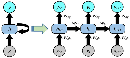
Figure 5.
PV power output for five different weather types.
Figure 6 shows the detailed process of the proposed ensemble forecasting algorithm. We take three-day ahead ensemble forecasting as an example to describe the detailed process. The input variables for the five single learners are preprocessed first. For each weather type, the original data set is split into training and testing sets to build up and test the single learners, respectively, i.e., ANN, DNN, SVR, LSTM, and CNN. The forecasting results of all the single learners are accounted as the ensemble input variables. The ensemble input variables are also split into training and testing sets for each weather type. The corresponding numbers of days for different weather types are shown in Table 2.
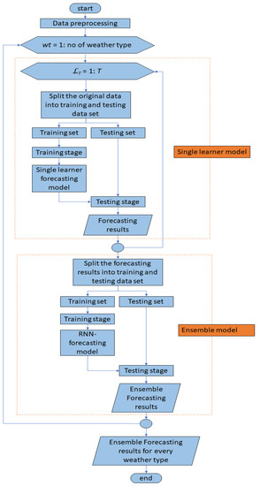
Figure 6.
The RNN structure.
Table 2.
The number of days in the training and testing stages.
4. Datasets and Performance Evaluation
This section introduces the data sets for training and testing, as well as the performance evaluation.
4.1. Datasets
In this study, the data were collected from the 200 kWp PV site of You Ji Industrial Co., Ltd. in Taiwan as installed at the building rooftop. In this research, the whole-year PV power output data in 2019 were collected.
The available data consisted of meteorological data and measured data from the PV site. The meteorological data were provided by Coastal Ocean Monitoring Center National Cheng Kung University (NCKU) Tainan, Taiwan. These data contained hourly weather predictions for three days ahead and updates every six hours per day at 00:00, 06:00, 12:00, and 18:00. Every time the weather predictions were updated every six hours, in this case, the newer weather prediction data overwrote the oldest. In other words, we only accepted the new data. The data features used in this study were hourly air temperature, relative humidity, and average wind speed. The actual measurement of hourly PV power output generated from each rooftop PV module of the building was also used as the data feature.
The correlation analysis was mainly used to select the proper data features. In this case, the Pearson correlation coefficient was used to calculate the correlation value between each variable, which had a value between −1 and 1 [4]. Table 3 shows the correlation coefficient, t statistics, and p values between weather variables and PV power output.
Table 3.
The statistical test between weather variables and PV power output.
Although the correlation coefficients of temperature, humidity, and wind speed were low, due to the t test results, the input variables with p values lower than 0.05 were still considered significant and used as input variables. In Reference [4], the use of temperature, humidity, and wind speed can give a lower error in irradiance forecasting, which is significantly related to PV power.
4.2. Training and Testing Sets
The data collected, as mentioned, were classified into five weather types based on the FCM clustering method and Calinski-Harabasz index. The weather types were sunny, light-cloudy, cloudy, heavy-cloudy, and rainy days.
The training and testing datasets of different weather types, as listed in Table 1, were used to train and test the single and ensemble learner, respectively. For the ensemble forecasting performance validation, the last three days of the testing data set were used in the ensemble model to perform one-day and three-day ahead PV power forecasting for each weather type. The detailed illustration of data preparation for the single learner and ensemble learner is described in Figure 7.
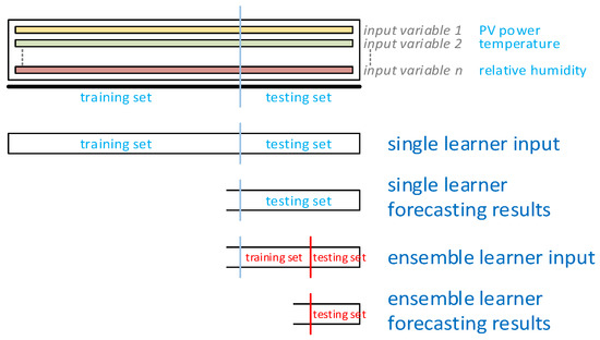
Figure 7.
The detailed process of the proposed ensemble forecasting algorithm.
4.3. Performance Evaluation
To verify the PV power prediction in this study, MRE was used as the main index to compare the performance of the different models. In MRE, the real and forecasting values were divided by the nominal capacity of the PV site, which was 200 kWp in our case, as computed below:
where and are the forecast value and true value of PV power output at ith point, respectively. N is the number of prediction points, and Np is the nominal power capacity of the PV site.
Performance evaluators, such as MRE, MAE, MAPE, RMSE, and R2 [47,48,49], were used to verify their forecasting method. In this work, it was necessary to evaluate the volatility of prediction error and the forecasting accuracy before we placed the results of several single learners into the ensemble model. Thus, we implemented performance evaluations such as MAE, nRMSE, and R2. MRE and MAE can represent the accuracy of the prediction. nRMSE can show the volatility or uncertainty condition of the prediction error. R2 is the predicted model coefficient of determination that lies between 0 and 1. A higher R2 leads to a smaller difference between the predicted and real value. MAE, nRMSE, and R2 are described in Equations (19)–(21), respectively.
5. Numerical Results
Short-term PV power forecasting covered the forecasting horizon up to 2–3 days ahead. In our case, we performed one-day and three-day ahead hourly PV power forecasting. One-day ahead PV power forecasting was applied in the applications of demand response, ancillary services, and unit commitment. For a longer-time horizon, three-day ahead PV power forecasting can be used practically for energy schedule, energy trading, and plant maintenance [50].
In this section, we conducted the simulations to verify our proposed ensemble forecasting model. MATLAB 2020a on Intel Core i7 3.60-GHz computer was employed for the simulation. As a comparison, the RF ensemble method was used as a benchmark model for one-day to three-day ahead PV power forecasting. As one of the supervised learning algorithms that consists of many decision trees and uses bagging, RF is considered the ensemble of decision trees by using bootstrap to subsample the input data and aggregation to combine the results. The detailed model of RF can be found in Reference [51].
5.1. Hyperparameter Setting of Single and Ensemble Models
Prediction performance was highly affected by hyperparameter tuning. Table 4 shows the parameters of five single forecasting models obtained by experiences related to the accuracy of every single model. Because the focus of this research was on the ensemble model, the single models were tuned without an optimization scheme to avoid the high computational cost.
Table 4.
Parameters of the single models.
The optimal hyperparameters tuned in the proposed ensemble model were defined by setting the number of the hidden layers, neurons, input delay, and learning rate. The hidden layer was set from 1 to 5, while the hidden neuron was set from 4 to 10. The input delay was set from 1 to 4, while the learning rate was 0.001, 0.005, 0.01, and 0.05. The benchmark RF model was tuned by setting the number of trees and minimal leaf size. The number of trees was 100, 500, and 1000 with minimal leaf sizes of 1, 3, 5, and 7. The optimal hyperparameters of the proposed ensemble model and benchmark model are shown in Table 5.
Table 5.
Optimal hyperparameters of the ensemble model.
5.2. Performance of The Proposed Ensemble Model
The FCM clustering method was performed to obtain the best number of clusters. Based on the CH index as shown in Figure 8, the maximum value was chosen as the optimal number of clusters. Therefore, the five clusters named sunny, light-cloudy, cloudy, heavy-cloudy, and rainy days, based on their characteristics were determined. On sunny days, the PV power output reached its maximum value. Cloudy days had medium PV power output, while on rainy days, the PV power output was low. Light-cloudy was between the sunny and cloudy days, while heavy-cloudy was between cloudy and rainy days. The overall weather types are shown in Figure 4.
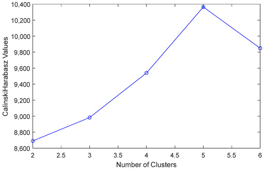
Figure 8.
Data preparation.
The proposed ensemble model was conducted using the stacking ensemble method via the meta-learner of RNN to combine the forecasting results of five single learners. First, we performed forecasting with every single learner by using training and testing datasets, as mentioned earlier. Second, the forecasting results from every single learner were used as training and testing datasets. The number of days for the ensemble learner and different weather types are shown in Table 1. There were 13, 23, 18, 14, and 7 days forecasting results for sunny, light-cloudy, cloudy, heavy-cloudy, and rainy days, respectively. The last three days of every weather type obtained from the single learner were used as the testing dataset for the ensemble learner, while the remaining days were used as the training dataset.
As shown in Table 5, for every weather type, the optimal hyperparameters of the RNN ensemble model had the same number of hidden layers and input delays. As the length of training and testing datasets was relatively short, up to 23 days, one hidden layer was sufficient to train the ensemble PV power forecasting model. The key difference of RNN performance as a meta-learner in PV power forecasting was in the number of hidden neurons related to the length of training and testing datasets. In light-cloudy and cloudy weather types, the number of hidden neurons was seven, which was the highest among the other weather types. The numbers of training and testing datasets in these two weather types were also the highest. Meanwhile, the lowest number of hidden neurons was the rainy weather type, which only had seven days of training and testing datasets. The RNN structure needed to be adjusted on the size of its hidden neurons to achieve a good fitting ability which led to an accurate forecasting model.
The comparison of predicted and actual values for one-day ahead PV power output between single and ensemble models is shown in Figure 9, Figure 10 and Figure 11 for sunny, cloudy, and rainy days. In terms of MRE as our main index, the MRE of DNN were 5.15%, 3.06%, and 9.11% on sunny, cloudy, and rainy days, respectively. On every weather type, DNN showed higher prediction performance than other single forecasting models based on the weighted average. ANN and LSTM showed lower prediction performance compared to the other methods. RNN ensemble achieved the best performance compared to RF and any single forecasting method with MRE of 4.70% on sunny days, while RF ensemble showed a good performance with MRE of 2.42% on cloudy days.
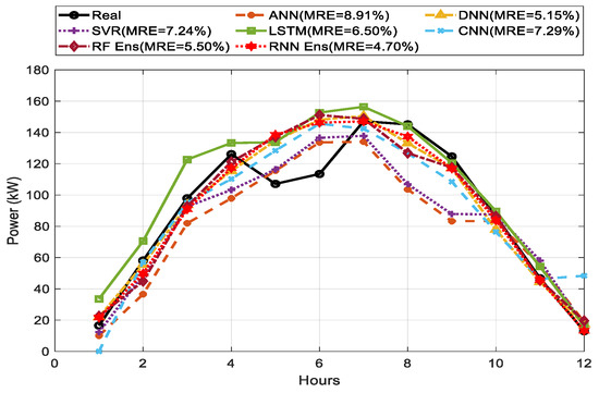
Figure 9.
Clustering optimization using Calinski-Harabasz index.
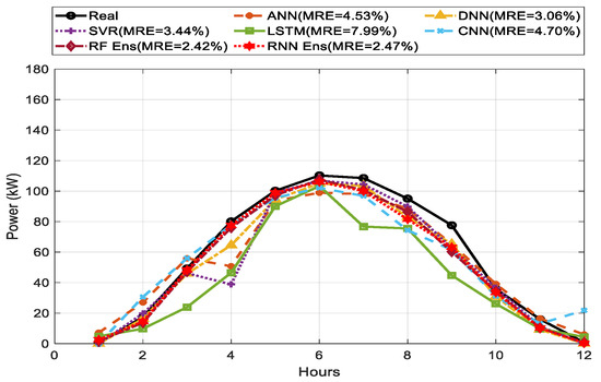
Figure 10.
One-day ahead PV power forecasting results for sunny days between single model and ensemble model.
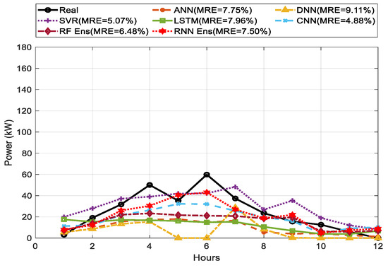
Figure 11.
One-day ahead PV power forecasting results for cloudy days between single model and ensemble model.
Figure 12, Figure 13 and Figure 14 show the comparison among the predicted and actual values of three-day ahead PV power output for weather types of sunny, cloudy, and rainy days. The weighted average of DNN showed the best prediction performance on every weather type compared to the other single forecasting models.
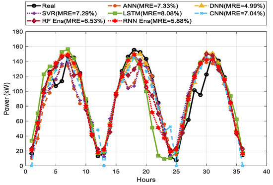
Figure 12.
One-day ahead PV power forecasting results for rainy days between single model and ensemble model.
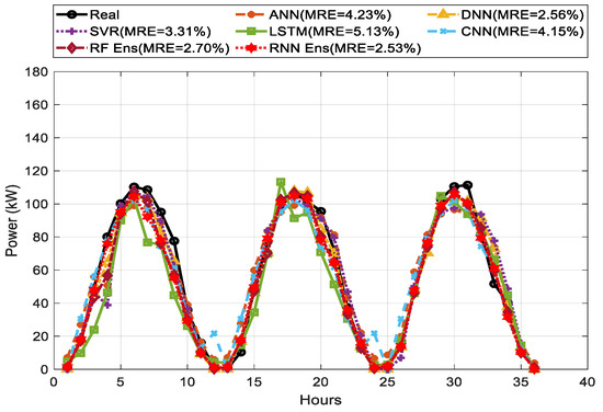
Figure 13.
Three-day ahead PV power forecasting results for sunny days between single model and ensemble model.
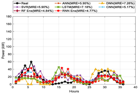
Figure 14.
Three-day ahead PV power forecasting results for cloudy days between single model and ensemble model.
LSTM and CNN showed the lowest performance. The MREs were 4.99%, 2.56%, and 7.26% for DNN on sunny, cloudy, and rainy days, respectively. DNN performed better than any single methods and ensemble methods with an MRE of 4.99% on sunny days. However, the RNN ensemble, as our proposed method, showed a consistent performance with the lowest MRE of 2.53% and 4.77% on cloudy and rainy days, respectively.
Table 6 shows the performance of the single and proposed ensemble method in one-day ahead forecasting with different error validations. As observed, the performance of our proposed method compares to the RF ensemble method on one-day ahead PV power forecasting. The weighted average MRE of the proposed RNN-ensemble method and the RF method were 3.87% and 4.53%, respectively. The proposed ensemble method is better, especially if the number of data points is low. RF only has a good prediction on cloudy days because RF can perform better on a higher number of data points for one-day ahead PV power forecasting. Overall, the superiority of our proposed method is prominent.
Table 6.
One-day ahead hourly forecasting performance.
Several single models were able to produce good results for certain weather types. However, they cannot perform well in all situations because every single method has its advantages. The proposed ensemble method can combine these advantages of a single method into a better result in terms of MRE, nRMSE, MAE, and R2.
Table 7 shows the performance evaluation index comparison for three-day ahead PV power forecasting between single and ensemble methods. The weighted average MRE of the proposed RNN ensemble method and the RF method were 4.29% and 4.68%, respectively. RF showed a good result on heavy-cloudy days since RF had the ability to reduce the variance part of error versus the bias in the heavy-cloudy dataset. Nevertheless, the proposed RNN ensemble method performed with more consistent accuracy, as shown on sunny, light-cloudy, cloudy, and rainy datasets over the RF, proving that the proposed RNN ensemble method is better than RF in forecasting time series data.
Table 7.
Three-day ahead hourly forecasting performance.
Although every single method and ensemble method can show their prediction ability for longer time horizons, the weighted average prediction for each weather type of the proposed ensemble method performed better than the benchmark and single methods. The overall comparison between one-day ahead and three-day ahead PV power forecasting shows that the proposed ensemble method can have consistency in terms of MRE, nRMSE, and MAE because the accuracy mismatch is relatively small, except for R2, which shows a lower prediction accuracy in three-day ahead forecasting than in one-day ahead forecasting.
In addition, to compare the proposed method with the different combinations of fewer single learner methods, the best three methods, DNN, SVR, and ANN, based on the lowest MRE, nRMSE, and MAE in Table 7, were chosen in this paper.
Table 8 and Table 9 show the comparison of the MRE and MAE among the combinations of the best three single learner methods, DNN+SVR, DNN+ANN, SVR+ANN, and DNN+SVR+ANN, and the proposed complete five single learner methods with RNN ensemble and DNN+SVR+ANN+LSTM+CNN, for three-day ahead hourly PV power forecasting. In the tables, the weighted results of all the methods are based on the number of days for each weather type.
Table 8.
Three-day ahead hourly forecasting performance (MRE) for different combinations of the single model in percentage.
Table 9.
Three-day ahead hourly forecasting performance (MAE) for different combinations of the single model in kW.
Figure 15 shows the comparison among the single methods with corresponding combinations of the best three, benchmark, and proposed methods in terms of the weighted average MRE and MAE. The combinations of the best three methods of DNN, SVR, and ANN are superior to any single method. The RNN-ensemble of DNN+SVR+ANN has slightly better accuracy than the benchmark method. The proposed method is proved that the RNN-ensemble of the five single learner methods is superior compared to the combinations of the best three single learner methods with MRE of 4.29% and MAE of 8.59 kW for a 200 kWp PV farm.
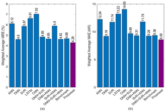
Figure 15.
Three-day ahead PV power forecasting results for rainy days between single model and ensemble model.
Furthermore, to evaluate the MAE’s improvement of the proposed method compared to the single, combinations of fewer singles via RNN ensemble, and benchmark method, Equations (22) and (23) are used below [52,53]:
where and are the MAE of the single, combinations of fewer singles, or benchmark method and the proposed method, respectively. is the difference between and .
The overall results are shown in Table 10. The proposed method had significant improvements by about 7–40% and 7–30% compared to the single models and the combinations of single models, respectively. As compared to the benchmark model, an 8% improvement was obtained.
Table 10.
The improvement of the proposed method compared to the single, combination, and benchmark methods.
The performance of both RF and RNN depended on time-series data processing. RF performed well only in tabular data. RF performance decreased in multivariate time series data. Although RNN had difficulty in predicting long-term dependencies, it was good at predicting sequential data with any length. Thus, the overall results show that our proposed method outperforms all single and benchmark methods.
6. Conclusions
In this paper, a stacking ensemble method with RNN as a meta-learner was proposed to improve the prediction accuracy for one-day to three-day ahead PV power forecasting. The forecasting results of ANN, DNN, SVR, LSTM, and CNN were combined by the RNN meta-learner to construct the ensemble model. Our proposed method is compared with the well-known benchmark ensemble model of random forest. This paper also compared the RNN-ensemble combination of the three best single learner methods using DNN, SVR, and ANN. Through intensive experiment, we found that the proposed ensemble method with the clustering method can outperform the single learner, the combinations of the single learners, and the benchmark ensemble method in terms of MRE, nRMSE, MAE, and R2. The proposed method reached the lowest MRE of 4.29%, which is a significant improvement for about 7–40%, 7–30%, and 8% as compared to the single models, the combinations of fewer single learners, and the benchmark method, respectively. Furthermore, the results show that the proposed ensemble method is reliable enough to be implemented in practical industrial applications.
The proposed method does not have as good accuracy in heavy-cloudy and rainy days as the other day types, as indicated by the coefficient of determination R2. Similar to many existing studies, these weather types are harder to predict accurately. Part of the reason is too little training data for these two types of weather to train the corresponding models. In future applications, it should be helpful to consider more weather variables that have a high correlation to PV power, such as cloudiness level [54] and irradiance data, to increase the accuracy of the proposed model. In addition to the random forest method, the other ensemble forecasting methods such as weighted averaging and ridge regression techniques [24] can also be used for comparison. Furthermore, the combination of the other machine learning methods can be studied to establish an ensemble method.
Author Contributions
This paper is a collaborative work of all authors. Conceptualization, A.A.H.L.; methodology, A.A.H.L., H.A., C.-Y.H., J.-L.Z. and N.H.P.; validation, A.A.H.L., H.-T.Y. and C.-M.H.; writing—original draft preparation, A.A.H.L.; supervision, H.-T.Y. and C.-M.H.; funding acquisition, A.A.H.L., H.-T.Y. and C.-M.H. All authors have read and agreed to the published version of the manuscript.
Funding
This research was funded by the Ministry of Science and Technology, Taiwan, under the grants MOST 110-3116-F-006-001.
Institutional Review Board Statement
Not applicable.
Informed Consent Statement
Not applicable.
Data Availability Statement
Not applicable.
Conflicts of Interest
The authors declare no conflict of interest.
References
- Kumar, N.; Singh, B.; Panigrahi, B.K.; Chakraborty, C.; Suryawanshi, H.M.; Verma, V. Integration of Solar PV With Low-Voltage Weak Grid System: Using Normalized Laplacian Kernel Adaptive Kalman Filter and Learning Based InC Algorithm. IEEE Trans. Power Electron. 2019, 34, 10746–10758. [Google Scholar] [CrossRef]
- Bag, A.; Subudhi, B.; Ray, P.K. A combined reinforcement learning and sliding mode control scheme for grid integration of a PV System. CSEE J. Power Energy Syst. 2019, 5, 498–506. [Google Scholar]
- Pradhan, S.; Hussain, I.; Singh, B.; Panigrahi, B.K. Performance Improvement of Grid-Integrated Solar PV System Using DNLMS Control Algorithm. IEEE Trans. Ind. Appl. 2019, 55, 78–91. [Google Scholar] [CrossRef]
- Kim, G.G.; Choi, J.H.; Park, S.Y.; Bhang, B.G.; Nam, W.J.; Cha, H.L.; Park, N.; Ahn, H.K. Prediction Model for PV Performance with Correlation Analysis of Environmental Variables. IEEE J. Photovolt. 2019, 9, 832–841. [Google Scholar] [CrossRef]
- Zhong, J.; Liu, L.; Sun, Q.; Wang, X. Prediction of Photovoltaic Power Generation Based on General Regression and Back Propagation Neural Network. Energy Procedia 2018, 152, 1224–1229. [Google Scholar] [CrossRef]
- Chen, B.; Lin, P.; Lai, Y.; Cheng, S.; Chen, Z.; Wu, L. Very-Short-Term Power Prediction for PV Power Plants Using a Simple and Effective RCC-LSTM Model Based on Short Term Multivariate Historical Datasets. Electronics 2020, 9, 289. [Google Scholar] [CrossRef] [Green Version]
- Catalina, A.; Alaiz, C.M.; Dorronsoro, J.R. Combining Numerical Weather Predictions and Satellite Data for PV Energy Nowcasting. IEEE Trans. Sustain. Energy 2020, 11, 1930–1937. [Google Scholar] [CrossRef]
- Li, Y.; Su, Y.; Shu, L. An ARMAX model for forecasting the power output of a grid connected photovoltaic system. Renew. Energy 2014, 66, 78–89. [Google Scholar] [CrossRef]
- Zhen, Z.; Pang, S.; Wang, F.; Li, K.; Li, Z.; Ren, H.; Shafie-khah, M.; Catalao, J.P.S. Pattern Classification and PSO Optimal Weights Based Sky Images Cloud Motion Speed Calculation Method for Solar PV Power Forecasting. IEEE Trans. Ind. Appl. 2019, 55, 3331–3342. [Google Scholar] [CrossRef]
- Akhter, M.N.; Mekhilef, S.; Mokhlis, H.; Mohamed Shah, N. Review on forecasting of photovoltaic power generation based on machine learning and metaheuristic techniques. IET Renew. Power Gener. 2019, 13, 1009–1023. [Google Scholar] [CrossRef] [Green Version]
- Li, G.; Xie, S.; Wang, B.; Xin, J.; Li, Y.; Du, S. Photovoltaic Power Forecasting with a Hybrid Deep Learning Approach. IEEE Access 2020, 8, 175871–175880. [Google Scholar] [CrossRef]
- Huang, C.J.; Kuo, P.H. Multiple-Input Deep Convolutional Neural Network Model for Short-Term Photovoltaic Power Forecasting. IEEE Access 2019, 7, 74822–74834. [Google Scholar] [CrossRef]
- Shi, J.; Lee, W.J.; Liu, Y.; Yang, Y.; Wang, P. Forecasting Power Output of Photovoltaic Systems Based on Weather Classification and Support Vector Machines. IEEE Trans. Ind. Appl. 2012, 48, 1064–1069. [Google Scholar] [CrossRef]
- Meng, M.; Song, C. Daily Photovoltaic Power Generation Forecasting Model Based on Random Forest Algorithm for North China in Winter. Sustainability 2020, 12, 2247. [Google Scholar] [CrossRef] [Green Version]
- Sanjari, M.J.; Gooi, H.B. Probabilistic Forecast of PV Power Generation Based on Higher Order Markov Chain. IEEE Trans. Power Syst. 2017, 32, 2942–2952. [Google Scholar] [CrossRef]
- Chen, B.; Li, J. Combined probabilistic forecasting method for photovoltaic power using an improved Markov chain. IET Gener. Transm. Distrib. 2019, 13, 4364–4373. [Google Scholar] [CrossRef]
- Ahmed Mohammed, A.; Aung, Z. Ensemble Learning Approach for Probabilistic Forecasting of Solar Power Generation. Energies 2016, 9, 1017. [Google Scholar] [CrossRef]
- Son, J.; Park, Y.; Lee, J.; Kim, H. Sensorless PV Power Forecasting in Grid-Connected Buildings through Deep Learning. Sensors 2018, 18, 2529. [Google Scholar] [CrossRef] [Green Version]
- Wan, C.; Zhao, J.; Song, Y.; Xu, Z.; Lin, J.; Hu, Z. Photovoltaic and solar power forecasting for smart grid energy management. CSEE J. Power Energy Syst. 2015, 1, 38–46. [Google Scholar] [CrossRef]
- Qiu, X.; Zhang, L.; Ren, Y.; Suganthan, P.; Amaratunga, G. Ensemble deep learning for regression and time series forecasting. In Proceedings of the 2014 IEEE Symposium on Computational Intelligence in Ensemble Learning (CIEL), Orlando, FL, USA, 9–12 December 2014; pp. 1–6. [Google Scholar]
- Eom, H.; Son, Y.; Choi, S. Feature-Selective Ensemble Learning-Based Long-Term Regional PV Generation Forecasting. IEEE Access 2020, 8, 54620–54630. [Google Scholar] [CrossRef]
- Raza, M.Q.; Mithulananthan, N.; Li, J.; Lee, K.Y.; Gooi, H.B. An Ensemble Framework for Day-Ahead Forecast of PV Output Power in Smart Grids. IEEE Trans. Ind. Inform. 2019, 15, 4624–4634. [Google Scholar] [CrossRef] [Green Version]
- Al-Dahidi, S.; Ayadi, O.; Alrbai, M.; Adeeb, J. Ensemble Approach of Optimized Artificial Neural Networks for Solar Photovoltaic Power Prediction. IEEE Access 2019, 7, 81741–81758. [Google Scholar] [CrossRef]
- Pan, C.; Tan, J. Day-Ahead Hourly Forecasting of Solar Generation Based on Cluster Analysis and Ensemble Model. IEEE Access 2019, 7, 112921–112930. [Google Scholar] [CrossRef]
- Liu, J.; Fang, W.; Zhang, X.; Yang, C. An Improved Photovoltaic Power Forecasting Model with the Assistance of Aerosol Index Data. IEEE Trans. Sustain. Energy 2015, 6, 434–442. [Google Scholar] [CrossRef]
- Yang, H.T.; Huang, C.M.; Huang, Y.C.; Pai, Y.S. A Weather-Based Hybrid Method for 1-Day Ahead Hourly Forecasting of PV Power Output. IEEE Trans. Sustain. Energy 2014, 5, 917–926. [Google Scholar] [CrossRef]
- Chai, M.; Xia, F.; Hao, S.; Peng, D.; Cui, C.; Liu, W. PV Power Prediction Based on LSTM With Adaptive Hyperparameter Adjustment. IEEE Access 2019, 7, 115473–115486. [Google Scholar] [CrossRef]
- Yu, Y.; Cao, J.; Zhu, J. An LSTM Short-Term Solar Irradiance Forecasting Under Complicated Weather Conditions. IEEE Access 2019, 7, 145651–145666. [Google Scholar] [CrossRef]
- Aprillia, H.; Yang, H.T.; Huang, C.M. Short-Term Photovoltaic Power Forecasting Using a Convolutional Neural Network–Salp Swarm Algorithm. Energies 2020, 13, 1879. [Google Scholar] [CrossRef]
- Ahmad, M.W.; Mourshed, M.; Rezgui, Y. Tree-based ensemble methods for predicting PV power generation and their comparison with support vector regression. Energy 2018, 164, 465–474. [Google Scholar] [CrossRef]
- Zhou, Z.H. Introduction. In Ensemble Methods: Foundations and Algorithms; Taylor & Francis: Boca Raton, FL, USA, 2012; pp. 1–21. [Google Scholar]
- Zhou, Z.H. Combination Methods. In Ensemble Methods: Foundations and Algorithms; Taylor & Francis: Boca Raton, FL, USA, 2012; pp. 67–97. [Google Scholar]
- Zhou, Z.H. Bagging. In Ensemble Methods: Foundations and Algorithms; Taylor & Francis: Boca Raton, FL, USA, 2012; pp. 47–66. [Google Scholar]
- Zhou, Z.H. Boosting. In Ensemble Methods: Foundations and Algorithms; Taylor & Francis: Boca Raton, FL, USA, 2012; pp. 23–46. [Google Scholar]
- Liu, H.; Tian, H.Q.; Li, Y.F.; Zhang, L. Comparison of four Adaboost algorithm based artificial neural networks in wind speed predictions. Energy Convers. Manag. 2015, 92, 67–81. [Google Scholar] [CrossRef]
- Ben Taieb, S.; Hyndman, R. A gradient boosting approach to the Kaggle load forecasting competition. Int. J. Forecast. 2014, 30, 382–394. [Google Scholar] [CrossRef] [Green Version]
- Fan, J.; Wang, X.; Wu, L.; Zhou, H.; Zhang, F.; Yu, X.; Lu, X.; Xiang, Y. Comparison of Support Vector Machine and Extreme Gradient Boosting for predicting daily global solar radiation using temperature and precipitation in humid subtropical climates: A case study in China. Energy Convers. Manag. 2018, 164, 102–111. [Google Scholar] [CrossRef]
- Park, J.; Moon, J.; Jung, S.; Hwang, E. Multistep-Ahead Solar Radiation Forecasting Scheme Based on the Light Gradient Boosting Machine: A Case Study of Jeju Island. Remote Sens. 2020, 12, 2271. [Google Scholar] [CrossRef]
- Li, Z.; Bao, S.; Gao, Z. Short Term Prediction of Photovoltaic Power Based on FCM and CG-DBN Combination. J. Electr. Eng. Technol. 2019, 15, 333–341. [Google Scholar] [CrossRef]
- Siddiqi, U.F.; Sait, S.M. A New Heuristic for the Data Clustering Problem. IEEE Access 2017, 5, 6801–6812. [Google Scholar] [CrossRef]
- Khashei, M.; Bijari, M. An artificial neural network (p,d,q) model for timeseries forecasting. Expert Syst. Appl. 2010, 37, 479–489. [Google Scholar] [CrossRef]
- Warsito, B.; Santoso, R.; Yasin, H. Cascade Forward Neural Network for Time Series Prediction. J. Phys. Conf. Ser. 2018, 1025, 012097. [Google Scholar] [CrossRef]
- Smola, A.J.; Schölkopf, B. A tutorial on support vector regression. Stat. Comput. 2004, 14, 199–222. [Google Scholar] [CrossRef] [Green Version]
- Hochreiter, S.; Schmidhuber, J. Long Short-Term Memory. Neural Comput. 1997, 9, 1735–1780. [Google Scholar] [CrossRef]
- Kuo, C.C.J. Understanding convolutional neural networks with a mathematical model. J. Vis. Commun. Image Represent. 2016, 41, 406–413. [Google Scholar] [CrossRef] [Green Version]
- Sehovac, L.; Grolinger, K. Deep Learning for Load Forecasting: Sequence to Sequence Recurrent Neural Networks with Attention. IEEE Access 2020, 8, 36411–36426. [Google Scholar] [CrossRef]
- Perveen, G.; Rizwan, M.; Goel, N. Comparison of intelligent modelling techniques for forecasting solar energy and its application in solar PV based energy system. IET Energy Syst. Integr. 2019, 1, 34–51. [Google Scholar] [CrossRef]
- Huang, Y.C.; Huang, C.M.; Chen, S.J.; Yang, S.P. Optimization of Module Parameters for PV Power Estimation Using a Hybrid Algorithm. IEEE Trans. Sustain. Energy 2020, 11, 2210–2219. [Google Scholar] [CrossRef]
- Lee, W.; Kim, K.; Park, J.; Kim, J.; Kim, Y. Forecasting Solar Power Using Long-Short Term Memory and Convolutional Neural Networks. IEEE Access 2018, 6, 73068–73080. [Google Scholar] [CrossRef]
- Antonanzas, J.; Osorio, N.; Escobar, R.; Urraca, R.; Martinez-de-Pison, F.J.; Antonanzas-Torres, F. Review of photovoltaic power forecasting. Sol. Energy 2016, 136, 78–111. [Google Scholar] [CrossRef]
- Breiman, L. Random Forests. Mach. Learn. 2001, 45, 5–32. [Google Scholar] [CrossRef] [Green Version]
- VanDeventer, W.; Jamei, E.; Thirunavukkarasu, G.S.; Seyedmahmoudian, M.; Soon, T.K.; Horan, B.; Mekhilef, S.; Stojcevski, A. Short-term PV power forecasting using hybrid GASVM technique. Renew. Energy 2019, 140, 367–379. [Google Scholar] [CrossRef]
- Leva, S.; Nespoli, A.; Pretto, S.; Mussetta, M.; Ogliari, E.G. PV Plant Power Nowcasting: A Real Case Comparative Study with an Open Access Dataset. IEEE Access 2020, 8, 194428–194440. [Google Scholar] [CrossRef]
- AccuWeather. Available online: https://www.accuweather.com/pl/tw/tainancity/314999/hourly-weather-forecast/314999 (accessed on 26 July 2021).
Publisher’s Note: MDPI stays neutral with regard to jurisdictional claims in published maps and institutional affiliations. |
© 2021 by the authors. Licensee MDPI, Basel, Switzerland. This article is an open access article distributed under the terms and conditions of the Creative Commons Attribution (CC BY) license (https://creativecommons.org/licenses/by/4.0/).