Abstract
Magnetic couplings (MCs) enable contactless speed/torque transmission via interactions between the magnetic fields of permanent magnets (PMs) rather than a physical mechanical connection. The contactless transmission of mechanical power leads to improvements in terms of efficiency and reliability due to the absence of wear between moving parts. One of the most common MC topologies is the coaxial type, also known as the radial configuration. This paper presents an analytical tool for the accurate and fast analysis of coaxial magnetic couplings (CMCs) using a two-dimensional subdomain approach. In particular, the proposed analytical tool resolves Laplace’s and Poisson’s equations for both air-gap and PM regions. The tool can be used to evaluate the impact of several design parameters on the performance of the CMC, enabling quick and accurate sensitivity analyses, which in turn guide the choice of design parameters. After discussing the building procedure of the analytical tool, its applicability and suitability for sensitivity analyses are assessed and proven with the analysis of a fully parameterized CMC geometry. The accuracy and the computational burden of the proposed analytical tool are compared against those of the finite element method (FEM), revealing faster solving times and acceptable levels of precision.
1. Introduction
MCs are used in applications where contactless torque/speed transmission is achieved by exploiting the magnetic interaction between both sides of the coupling. Contactless torque/speed transmission delivers substantial advantages in terms of low maintenance requirements, high efficiency, thermal isolation, and overload protection [1,2,3]. Furthermore, the absence of physical contact allows the blockage or separation of the magnetic connection between prime mover and load sides [4]. Thus, the power transmission can be inhibited in case of failure, providing inherent overload protection that allows for safe operation under excessive load conditions, which might otherwise lead to catastrophic failures. Although MCs possess significant advantages over existing mechanical couplings, research is still ongoing, and care is required in their design and operation [5,6]. They may need soft staring conditions or very low inertia systems to avoid critical speeds and prevent rotor resonance, which would lead to excessive torsional loading [7,8]. Therefore, it is critical to ensure appropriate torque capacity is achieved in MCs by analyzing their design parameters in a fast and accurate manner.
One of the most effective numerical analysis methods, the finite element method (FEM), is widely used in rotating electrical machine design [9] and similar fields [10]. Currently available commercial software (e.g., MagNet, Flux, ANSYS, COMSOL, JMAG, etc.) enables the resolution of complex models for performance analysis of electrical motors, generators, MCs and magnetic gearboxes. Some of them feature more advanced coding with improved discretization of models such as meshing with h-adaptive elements and by considering elements up to the fifth order [11,12]. FEM allows accurate computation of air-gap field and torque [13,14,15,16]. However, in cases where a study needs to be evaluated with a wide range of size parameters, the FEM becomes more complex and time consuming than evaluating by analytical methods [17,18]. Therefore, analytical methods are helpful analysis tools for the first step of the design process (i.e., trade-off studies and sensitivity analyses) as they can be used to rapidly obtain a solution. Previously, the COMPUMAG TEAM benchmark problem 30a is solved by analytical method. The method is suggested due to challenges that finite element approaches were not capable of resolving with respect to rotational induced eddy currents [19]. The problem was later solved by the boundary element method and by the time-harmonic FEM [20]. A two-dimensional (2D) analytical model by subdomain analysis was introduced by Thierry et al. [21]. The model was developed for an axial MC for an exact analytical solution of the magnetic field distribution and electromagnetic torque. Due to model simplifications in changing the geometry from 3D to 2D by considering an unrolled cylindrical cutting surface, the torque results see a significant mismatch with the experimental results. However, the analytical approach discussed in [21] is suitable for the preliminary design and sizing of an axial MC. In [22], the MC detailed in [21] is investigated to observe its steady state and transient performance. The experimental study of same axial MC is debated in [23] along with the investigation on the effects of misalignment between the motor and load side of the MC. In [24], one side of the axial MC is replaced with copper material to develop an axial-field eddy-current coupling. The resulting eddy currents are analytically evaluated using a 2D model. The research on the axial-field eddy-current coupling is further improved by introducing the 3D analytical method in [25].
The mentioned papers, i.e., [21,22,23,24,25], show that in the literature there is a relatively high availability of research on MCs featuring an axial configuration, although the same cannot be asserted for the coaxial topology. The first considerable study on the coaxial configuration was presented in [26], where the static torque distribution of the CMC is plotted by considering different numbers of pole pairs. Furthermore, the effects of the air-gap thickness on the CMC have been investigated through 2D and 3D FEMs in [27] and the obtained results are compared against experimental findings. Finally, the performance of the CMC equipped with NdFeB rare earth PMs has been assessed in [28].
For both axial and coaxial MCs [29], the research works available in literature mainly focus on the performance impact of a single size parameter, although more effective design choices could be made by taking into account several design parameters, such as the number of pole pairs, PM thickness, air-gap thickness, etc. To achieve a more comprehensive preliminary design capability, it would be essential to rely on a fast and accurate analysis tool.
In response to such a need, the paper introduces a 2D analytical tool capable of computing both the air-gap field distribution and the transmitted torque in order to assess the CMC performance. Firstly, the building procedure and the fundamental equations for the tool are detailed. Then, the analytical tool is used to analyze a variety of size parameters as would be required during the preliminary design of a CMC. The benefits of the proposed approach in terms of both computation time and accuracy are evaluated against FEM outcomes. As expected, the analytical tool features excellent solving time and its accuracy is more than acceptable for the purpose of a sensitivity study. These two strengths prove the feasibility and effectiveness of the preliminary design tool.
2. Development and Validation of the 2D Analytical Tool
This section deals with the fundamental equations and the boundary conditions of each subdomain of the CMC architecture. Once the proposed 2D analytical tool is built, an arbitrary fully parametric CMC geometry is chosen and validated with results obtained from the FEM. The analytical method employed in this paper is based on the resolution of the Laplace’s and Poisson’s equations in the air-gap and PM subdomains respectively. Figure 1 outlines the CMC which is comprised of three subdomains. These are the inner ring and outer ring PM subdomains (region I and III), and the air-gap subdomain (region II). The numerical values reported in Table 1 refer to the CMC geometry adopted for comparing analytical and FEM initial outcomes. It should be noted that the parameters listed in Table 1 are procured from one of the cases detailed in Section 3 and the vector potentials are solved in polar coordinate.
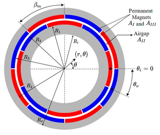
Figure 1.
Outline of the CMC.

Table 1.
CMC parameters used in the validation exercise.
The 2D analytical method is developed under following assumptions [30]:
- End effects are neglected due to the cylindrical geometry.
- Permeability of the back iron is infinite. Hence, the magnetic field is perpendicular to the back iron.
- Relative permeability of the PMs is taken as 1.
- PMs are radially magnetized.
For MC PMs, assuming a ferromagnetic material with infinite permeability (i.e., the magnetic saturation is neglected) is fair, since they do not suffer from the same armature reaction effect as electrical machines and unlike magnetic gearboxes, the portion of ferromagnetic material facing the air-gap is limited.
According to the polar coordinate adoption, the vector potentials for each subdomain have only z-directional components which depend on and (i.e., radial distance and angle respectively). Thus, the magnetic vector potential for each subdomain is represented by the following notations.
2.1. Potential Functions
Figure 2 shows the air-gap subdomain and the related boundary conditions. The general solution of the air-gap region potential function is given by (1).
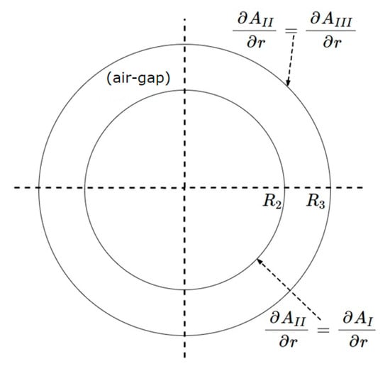
Figure 2.
The air-gap subdomain and its boundary conditions.
The boundary conditions, which define the behavior of the magnetic fields between different materials for the air-gap subdomain, are expressed in (2) and (3).
Given the air-gap subdomain boundary conditions, Equation (1) is characterized as detailed in (4).
where , , and are the coefficients of the vector potential determined by using the relationship between the boundary conditions and the potential functions that, for the sake of completeness, are reported in Appendix A. The potential functions are then employed to create a Fourier series expansion and determine the coefficients. The notation n represents a positive integer.
The potential equation for the PM regions is developed by the resolution of the Poisson’s equation as shown in (5).
where and are the vector potentials for the inner and outer PMs, respectively and is the radial magnetization of the PMs. The magnetization vector is represented by the expression provided in (6) with as the permeability of free space and as the remanent magnetization.
In terms of polar coordinates, is expressed according to (7), where and denote the direction vectors in the radial and tangential directions, while and denote the components’ magnitudes, as depicted in Figure 3.
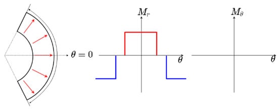
Figure 3.
Magnetization components for radially magnetized PMs.
The PMs in the analytical models are represented with a Fourier series expansion of their magnetization. As previously mentioned, the magnetization pattern is assumed to be radial. Different types of magnetization patterns, such as parallel or Halbach array, can be found in [31,32]. The general solution for the inner PM subdomain is given in (8).
where , , and are the coefficients of the vector potential, is the initial angle of the inner PM, and is defined in (9).
For the inner PM region, the boundary conditions are illustrated in Figure 4 while their mathematical expression is formalized in (10) and (11).
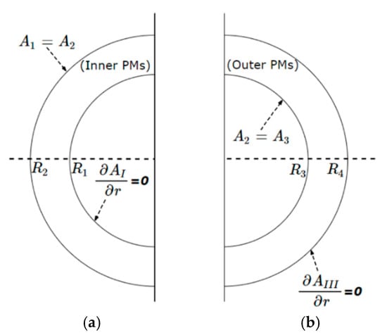
Figure 4.
The PM subdomains and their boundary conditions; (a) Inner PM region, (b) Outer PM region.
Similarly, the vector potential for the outer PM is determined according to (12).
where , , and are the coefficients of the vector potential, is the initial angle of the outer PM, and is calculated based on (13).
Considering the outer PM region, its boundary conditions are described by (14) and (15) and visualized in Figure 4 for the sake of completeness.
2.2. Flux Density and Static Torque
Knowing the solutions of the vector potential in the air-gap, the corresponding flux density distribution is determined as in (16) and (17).
Rearranging (16) and (17), the components of the flux density distribution can also be expressed through (18) and (19).
Finally, the transmitted torque is calculated by using the Maxwell stress tensor method, as shown in (20), where represents the mean radius for the integration within the air-gap region.
2.3. Validation Exercise
In this subsection, a comparative exercise between the 2D analytical method and 2D FEM is performed for validation purposes and the obtained results are presented. The FEM simulations are carried out by using the software package Simcenter MagNet. The FEM analysis takes the polynomial orders (i.e., p-type adaption) as 2 for all cases in this paper and magnetic material properties are non-linear. In addition, the mesh refinement (i.e., h-type adaption) is considered until the maximum relative error is minimized.
The comparative exercise is carried out by taking the values given in Table 1. The back-iron and PM materials considered in the FEM are laminated silicon steel M530-50A (grade EN 10106) and NdFeB ( 1.29 T) respectively. The mesh edge subdivision is taken to be uniform. After applying the specified conditions, the flux lines and flux density map resulting from the 2D FEM are plotted in Figure 5. The highest magnetic saturation level is observed at the maximum torque point, which is an unstable operating point (small torque variations will cause slip in magnetic couplings). Under actual operating conditions, the magnetic coupling will transfer torque at a non-zero shift angle, therefore the transmitted toque is lower than the maximum torque. However it will feature a higher stability margin and a lower magnetic saturation level. For this reason, the assumption of infinite permeability is consistent with the actual operation conditions of the magnetic coupling.
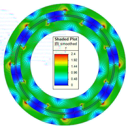
Figure 5.
Flux density distribution and flux lines at the maximum torque point.
At the maximum torque point, the local magnetic saturation mainly occurs near the PM edges (see Figure 5), while the air-gap magnetic field is not significantly affected by the magnetic saturation. In fact, a good match between 2D FEM and analytical results is obtained when the radial (i.e., Figure 6) and tangential (i.e., Figure 7) components of the flux density distribution in the air-gap are evaluated. Due to the magnetic saturation, the mismatch between 2D FEM and 2D analytical results in Figure 8 increases when the PMs are not aligned (i.e., the shift angle is non-zero and the maximum static torque is transferred). Indeed, a more significant local magnetic saturation is observable at the PM edges (see Figure 5) when the maximum static torque equilibrium point is considered. The relatively low error values for both flux density components and static torque prove the effectiveness of the 2D analytical tool.
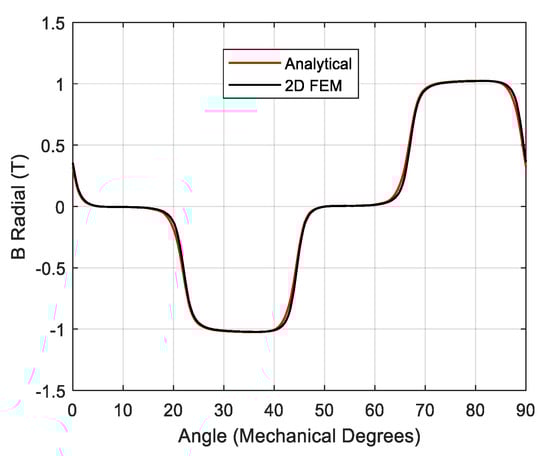
Figure 6.
Radial component of the flux density distribution at the maximum torque point: 2D FEM (black) and analytical (red).
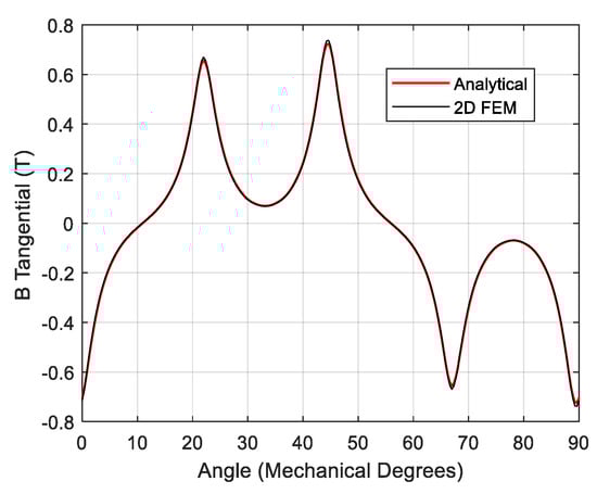
Figure 7.
Tangential component of the flux density distribution at the maximum torque point: 2D FEM (black) and analytical (red).
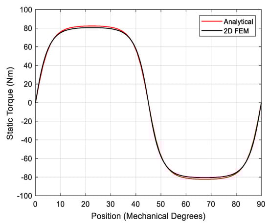
Figure 8.
Static torque: 2D FEM (black) and analytical (red).
3. Sensitivity Analyses and Computational Time Evaluation
Following validation of the 2D analytical tool in Section 2, its performance is further evaluated in terms of the required computational time compared to the FEM. It is worth pointing out that the accuracy evaluation (see Section 2.3) was performed considering the parameters listed in Table 1, while the computational time investigation is carried out based on the different CMC geometries whose parameters are given in Table 2. Indeed, different size parameters are selected and varied to emulate a sensitivity analysis typical of the preliminary design. In particular, the effects of the design parameters, such as pole pairs number, PM thickness, and the outer diameter of the CMC, on the computational time are analysed.
Table 2.
Parameters of the CMC considered during the sensitivity analysis.
One of the important parameters effecting the simulation and solving time is the number of pole pairs. It is widely known that increasing the number of pole-pairs requires the analysis of a greater number of harmonics in order to maintain accurate flux density plots and torque results [17], thus leading to an increase in the solving time. The first two cases of the sensitivity analysis (see Table 2) aim to compare the solving time between two CMC geometries, which feature four and sixteen pole pairs respectively, while the other geometric parameters are kept unchanged. By varying the number of pole-pairs, a greater impact on the solving time of the 2D analytical method is expected compared with that of the FEM.
In cases three and four of the sensitivity analysis, the air-gap thickness of the CMC is varied (see Table 2) and a fair comparison is achieved by carefully selecting the air-gap mesh size in the FEM, as discussed in Section 3.1. The variation in air-gap thickness has a greater impact on the FEM solving time.
In cases five and six of the sensitivity analysis, the active volume of the CMC is changed by adjusting both the inner radius of the back-iron (i.e., 150 mm instead of 35 mm) and the PM thicknesses (i.e., 20 mm and 30 mm respectively), as can be seen in Table 2.
Finally, case seven of the sensitivity analysis examines a full pole-pairs sweep ranging from 2 to 30, while maintaining the same geometric parameters. The maximum static torque is then calculated for each CMC geometry considered, along with the solving time for both the 2D analytical method and FEM. It is worth noting that the solving time required by the FEM also includes the time needed for building the simulated model.
3.1. Mesh Size Selection
In the FEM, the size of the mesh elements plays an important role in determining both the solution accuracy and the solving time [33]. Both quantities grow with smaller mesh elements. Thus, the mesh density should be increased only in important areas of the model, such as the air-gap, to avoid unnecessary computational burden. A trade-off analysis is performed with variable mesh density to obtain the most effective model solution whilst maintaining accurate results. In order to achieve this task, an index named “mesh-factor” h is introduced, which is a dimensionless variable that enables auto adjustment of the mesh size for each CMC region, i.e., air-gap, PMs, and back-iron. Therefore, the mesh-factor is changed accordingly to obtain the appropriate mesh density. Table 3 shows the specified CMC regions along with the corresponding mesh size values, which are expressed as function of the mesh-factor.
Table 3.
Mesh size selection method.
Figure 9 depicts the mesh map at different mesh-factor values (h), i.e., 10, 1, and 0.5, and the reported results refer to the CMC parameters of the first case given in Table 2.
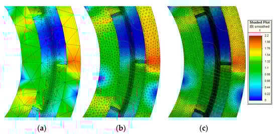
Figure 9.
The mesh map with mesh-factor of: (a) 10, (b) 1, (c) 0.5.
In terms of solution accuracy, the ‘optimal mesh-factor’ for FEM is identified by determining the maximum relative error. In particular, the CMC geometry described in case one of Table 2 is adopted as benchmark model and several mesh-factor values, ranging from 1 to 20, have been tested. The maximum error associated with each mesh factor value is calculated relative to the error resulting from the selection of a mesh-factor equal to 0.5 (i.e., the smallest value that leads to the most accurate solution that also requires the greatest computational time). The obtained error values are given in Figure 10, which shows that h = 3 delivers a relatively low error with reasonable computational effort. Hence, the mesh-factor h = 3 is selected for the FEM applied to case one of Table 2. For the remaining cases, a similar trade-off study has been performed to determine the ‘optimal mesh-factor’ value. The obtained results are listed in Table 4 along with the mesh size (expressed in mm) of every CMC part.
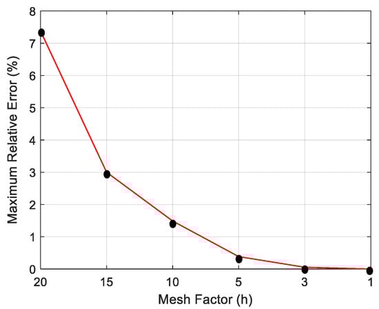
Figure 10.
Maximum relative error as function of the mesh-factor.
Table 4.
Mesh-factor and Mash size values.
3.2. Harmonic Numbers Selection
The 2D analytical tool that has been developed relies on the Fourier series expansion of the arbitrary constants of the general equations found by the resolution of the Laplace’s and Poisson’s equations (see Section 2). The air-gap field is produced by the PMs excitation due to their space harmonics and the 2D analytical tool accounts for just five harmonics in this work. Apart from the fundamental harmonic, which corresponds to the number of pole-pairs, another four harmonics are considered (e.g., for case one, the evaluated harmonics are 4, 12, 20, 28 and 36). Thus, the fundamental and the summation up to five harmonics is taken into account for every analysed CMC, as detailed in Table 5, where the harmonic values are made explicit. The MMF harmonics, when n = s. p with s = 1, 3, 5, 7, 9, and n pole-pairs number, create the air-gap field. Thus, the summation 4 in Table 5 simply takes the summation of the fundamental harmonic and 4 other following harmonics, which are 3rd, 5th, 7th, and 9th.
Table 5.
Selected harmonic numbers for the 2D analytical tool.
Referring to the values of Table 5, the CMC’s static torque has been calculated at different harmonic numbers via the 2D analytical tool and the results have been compared with those obtained through the FEM. For case one, the comparison outcomes are summarized in Figure 11, which reveals that the static torque associated with only the fundamental harmonic produces almost 20% of maximum relative error. Conversely, the maximum relative error decreases to 2.3% when the summation of all five harmonic components are evaluated.
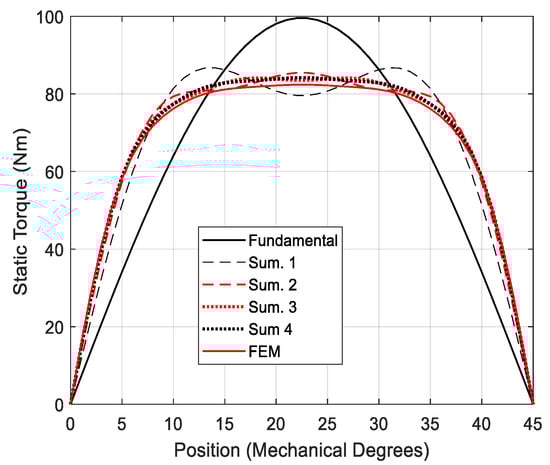
Figure 11.
Static torque comparison with different harmonic numbers and FEM, case one.
3.3. Results Comparison
Following determination of the ‘optimal’ value of the mesh-factor for the FEM and definition of the number of harmonics for the 2D analytical tool, the sensitivity analyses are performed for the 7 cases detailed in Table 2. The computational time comparison has been carried out on a Desktop PC running the Microsoft 10 operating system with an Intel Core i3 CPU @ 3.4 GHz with 2 cores. In terms of software, a Matlab m-file has been adopted to implement the developed analytical tool, while the finite element simulations are ran on the Simcenter MagNet FE software package. The results in terms of solving time and maximum relative error of the static torque are given in Table 6 for both 2D analytical tool and the FEM. It should be noted that the time values from case one to case six are relative to 46 samples of the static torque (i.e., 46 shift angle values), which are taken on half cycle (i.e., 180 electrical degrees). Analyzing case one, the 2D analytical method takes 32.8 s with a 3.1% error (calculated against the FEM static torque), while 240 s are required by the FEM. Hence, the developed analytical tool delivers the solution in approximately 87% less time than the FEM. For case one, the graphical comparison regarding the static torque trend is illustrated in Figure 11. On the other hand, case two considers the same size parameters as for case one, but with four times the number of pole-pairs (i.e., 16 instead of 4). The greater number of pole-pairs implies a longer solving time. Indeed, the solving time is equal to 31.2 s with a 3.8% error for the 2D analytical tool, whilst the FEM takes 401 s. In other words, a time saving of about 92% is achieved with the 2D analytical tool. For case two, the static torque trend comparison is shown in Figure 12.
Table 6.
Solving time and static torque maximum error.
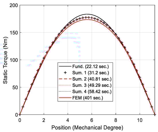
Figure 12.
Case two: Static torque comparison.
The effect of the air-gap thickness is addressed by cases three and four, where the CMCs feature 4 mm and 8 mm air-gap thickness respectively (i.e., twice and four times the air-gap thickness considered for the CMCs of the previous two cases). As expected, the solving time increases with increased air-gap thickness, although the 2D analytical method does not require a high number of harmonics as shown in Figure 13 (case four). In terms of solving time, 20.3 s and 665 s are respectively employed by the 2D analytical tool and the FEM, with an overall time saving of about 96%.
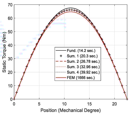
Figure 13.
Case four: Static torque comparison.
In cases five and six, the CMCs are characterized by a significantly larger volume compared to the previous cases. This aspect mainly affects the solving time of the FEM, since the 2D analytical method features almost the same time values as in cases three and four, although slightly less accurate results are obtained. The lowest relative error (about 2.6% average) is achieved when all five harmonics are summated, with a solving time reduction of about 97% (i.e., 27 s and 902 s for 2D analytical tool and FEM respectively on average).
In case seven, the CMC’s pole-pairs number is varied from 2 to 30, as would be required during a preliminary design sensitivity analysis. In order to complete this analysis, the 2D analytical tool demands 14.65 s, whereas 650 s are needed by the FEM (i.e., approximately a 97% time reduction). For the sake of completeness, the peak static torque comparison for up to 5 harmonics with the FEM is shown in Figure 14.
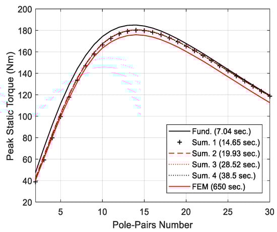
Figure 14.
Case seven: Comparison of the peak static torque as function of the pole-pairs number.
4. Conclusions
A 2D analytical tool has been developed by using a subdomain method. The proposed analytical tool takes resolutions of Laplace’s equations in the air-gap and Poisson’s equations in the PM subdomains. The air-gap flux density distribution and the static torque are calculated by the analytical tool and validated with a FEM. The validation results showed a good agreement, hence fast and accurate CMC analysis is achieved via the proposed tool. These features make the tool suitable for employment at the early design stage of a CMC, where several design parameters need to be evaluated for guiding the design choices.
A comprehensive sensitivity analysis has been carried out for evaluating both computational time and accuracy under the variation of design parameters (e.g., air-gap thickness, number of pole-pairs, etc.). Based on the presented findings, the proposed 2D analytical tool is characterized by a significantly shorter computational time than the FEM while ensuring a reasonable level of accuracy.
Author Contributions
Conceptualization, Y.A., P.G. and M.G.; methodology, Y.A. and P.G.; software, Y.A.; validation, O.T., P.G. and M.G.; formal analysis, P.G. and M.G.; investigation, Y.A and O.T.; resources, Y.A.; data curation, P.G. and M.G.; writing—original draft preparation, Y.A.; writing—review and editing, Y.A., O.T. and P.G.; visualization, O.T. and P.G; supervision, P.G. and M.G.; project administration, M.G.; funding acquisition, M.G. All authors have read and agreed to the published version of the manuscript.
Funding
This research was funded by the Clean Sky 2 Joint Undertaking under the European Union’s Horizon 2020 research and innovation programme, grant number 821023 and the Clean Sky 2 Joint Undertaking under the European Union’s Horizon 2020 research and innovation programme, grant number 807081.
Institutional Review Board Statement
Not applicable.
Informed Consent Statement
Not applicable.
Data Availability Statement
Not applicable.
Conflicts of Interest
The authors declare no conflict of interest.
Appendix A
Considering the boundary conditions at the air-gap (region II) given in (2) and (3), the following equation can be written:
From the boundary conditions in the PMs subdomains expressed by (10) and (11), the following equations can be derived:
The continuity of the PM and the air-gap subdomains leads to (A7) and (A8).
Rearranging (14), it is possible to obtain (A9) and (A10).
Finally, the boundary condition given by (14) results in (A11) and (A12).
The equations resulting from both boundary and interface conditions, i.e., (A1)–(A12), are organized in matrix form and then solved using linear equations in order to find the vector potential coefficients. The solution of the constants requires MATLAB software to be solved and the matrix form is written as shown in (A13).
Therefore, the complete matrix form is given by (A14).
References
- Wu, W.; Lovatt, H.; Dunlop, J. Analysis and design optimisation of magnetic couplings using 3D finite element modelling. IEEE Trans. Magn. 1997, 33, 4083–4094. [Google Scholar] [CrossRef]
- Galea, M.; Giangrande, P.; Madonna, V.; Buticchi, G. Reliability-Oriented Design of Electrical Machines: The Design Process for Machines’ Insulation Systems MUST Evolve. IEEE Ind. Electron. Mag. 2020, 14, 20–28. [Google Scholar] [CrossRef]
- Charpentier, J.-F.; Lemarquand, G. Study of permanent-magnet couplings with progressive magnetization using an analytical formulation. IEEE Trans. Magn. 1999, 35, 4206–4217. [Google Scholar] [CrossRef][Green Version]
- Kim, S.H.; Shin, J.W.; Ishiyama, K. Magnetic Bearings and Synchronous Magnetic Axial Coupling for the Enhancement of the Driving Performance of Magnetic Wireless Pumps. IEEE Trans. Magn. 2013, 50, 1–4. [Google Scholar] [CrossRef]
- Akcay, Y.; Giangrande, P.; Galea, M. A Novel Magnetic Coupling Configuration for Enhancing the Torque Density. In Proceedings of the 2020 23rd International Conference on Electrical Machines and Systems (ICEMS), Hamamatsu, Japan, 24–27 November 2020; pp. 228–233. [Google Scholar]
- Akcay, Y.; Giangrande, P.; Galea, M. Design, Analysis and Dynamic Performance of Radial Magnetic Coupling. In Proceedings of the 2020 23rd International Conference on Electrical Machines and Systems (ICEMS), Hamamatsu, Japan, 24–27 November 2020; pp. 222–227. [Google Scholar]
- Ho, S.L.; Niu, S.; Fu, W. Transient Analysis of a Magnetic Gear Integrated Brushless Permanent Magnet Machine Using Circuit-Field-Motion Coupled Time-Stepping Finite Element Method. IEEE Trans. Magn. 2010, 46, 2074–2077. [Google Scholar] [CrossRef]
- Giangrande, P.; Madonna, V.; Nuzzo, S.; Galea, M. Design of Fault-Tolerant Dual Three-Phase Winding PMSM for Helicopter Landing Gear EMA. In Proceedings of the 2018 IEEE International Conference on Electrical Systems for Aircraft, Railway, Ship Propulsion and Road Vehicles & International Transportation Electrification Conference (ESARS-ITEC), Nottingham, UK, 7–9 November 2018. [Google Scholar]
- Al-Timimy, A.; Degano, M.; Giangrande, P.; Calzo, G.L.; Xu, Z.; Galea, Z.X.M.; Gerada, C.; Zhang, H.; Xia, L. Design and optimization of a high power density machine for flooded industrial pump. In Proceedings of the 2016 XXII International Conference on Electrical Machines (ICEM), Lausanne, Switzerland, 4–7 September 2016; pp. 1480–1486. [Google Scholar]
- Giangrande, P.; Cupertino, F.; Pellegrino, G. Modelling of linear motor end-effects for saliency based sensorless control. In Proceedings of the 2010 IEEE Energy Conversion Congress and Exposition, Atlanta, GA, USA, 12–16 September 2010; pp. 3261–3268. [Google Scholar] [CrossRef]
- Karban, P.; Pánek, D.; Orosz, T.; Petrášová, I.; Doležel, I. FEM based robust design optimization with Agros and Ārtap. Comput. Math. Appl. 2021, 81, 618–633. [Google Scholar] [CrossRef]
- Kiss, G.M.; Kaska, J.; Oliveira, R.; Rubanenko, O.; Tóth, B. Performance Analysis of FEM Solvers on Practical Electromagnetic Problems. Period. Polytech. Electr. Eng. Comput. Sci. 2021, 65, 113–122. [Google Scholar] [CrossRef]
- Mezani, S.; Laporte, B.; Takorabet, N. Saturation and space harmonics in the complex finite element computation of induction motors. IEEE Trans. Magn. 2005, 41, 1460–1463. [Google Scholar] [CrossRef]
- Williamson, S.; Lim, L.; Smith, A. Transient analysis of cage-induction motors using finite-elements. IEEE Trans. Magn. 1990, 26, 941–944. [Google Scholar] [CrossRef]
- Williamson, S.; Lim, L.; Robinson, M. Finite-element models for cage induction motor analysis. IEEE Trans. Ind. Appl. 1990, 26, 1007–1017. [Google Scholar] [CrossRef]
- Coulomb, J. A methodology for the determination of global electromechanical quantities from a finite element analysis and its application to the evaluation of magnetic forces, torques and stiffness. IEEE Trans. Magn. 1983, 19, 2514–2519. [Google Scholar] [CrossRef]
- Lukic, M.; Hebala, A.; Giangrande, P.; Klumpner, C.; Nuzzo, S.; Chen, G.; Gerada, C.; Eastwick, C.; Galea, M. State of the Art of Electric Taxiing Systems. In Proceedings of the 2018 IEEE International Conference on Electrical Systems for Aircraft, Railway, Ship Propulsion and Road Vehicles & International Transportation Electrification Conference (ESARS-ITEC), Nottingham, UK, 7–9 November 2018. [Google Scholar]
- Giangrande, P.; Madonna, V.; Sala, G.; Kladas, A.; Gerada, C.; Galea, M. Design and Testing of PMSM for Aerospace EMA Applications. In Proceedings of the IECON 2018—44th Annual Conference of the IEEE Industrial Electronics Society, Washington, DC, USA, 21–23 October 2018; pp. 2038–2043. [Google Scholar]
- Davey, K.R. Analytic analysis of single- and three-phase induction motors. IEEE Trans. Magn. 1998, 34, 3721–3727. [Google Scholar] [CrossRef]
- Marcsa, D.; Kuczmann, M. Motion finite element simulation of a single-phase induction motor. Pollack Period. 2009, 4, 57–66. [Google Scholar] [CrossRef]
- Lubin, T.; Mezani, S.; Rezzoug, A. Simple Analytical Expressions for the Force and Torque of Axial Magnetic Couplings. IEEE Trans. Energy Convers. 2012, 27, 536–546. [Google Scholar] [CrossRef]
- Lubin, T.; Mezani, S.; Rezzoug, A. Steady-state and transient analysis of an axial-field magnetic coupling. In Proceedings of the 2012 XXth International Conference on Electrical Machines, Marseille, France, 2–5 September 2012; pp. 1443–1449. [Google Scholar]
- Lubin, T.; Mezani, S.; Rezzoug, A. Experimental and Theoretical Analyses of Axial Magnetic Coupling Under Steady-State and Transient Operations. IEEE Trans. Ind. Electron. 2013, 61, 4356–4365. [Google Scholar] [CrossRef]
- Lubin, T.; Rezzoug, A. Steady-State and Transient Performance of Axial-Field Eddy-Current Coupling. IEEE Trans. Ind. Electron. 2014, 62, 2287–2296. [Google Scholar] [CrossRef]
- Lubin, T.; Rezzoug, A. 3-D Analytical Model for Axial-Flux Eddy-Current Couplings and Brakes under Steady-State Conditions. IEEE Trans. Magn. 2015, 51, 1–12. [Google Scholar] [CrossRef]
- Nagrial, M. Analysis, design and performance of magnetic couplings. In Proceedings of the 1995 International Conference on Power Electronics and Drive Systems. PEDS 95, Singapore, 21–24 February 1995; Volume 2, pp. 634–638. [Google Scholar]
- Yao, Y.; Huang, D.; Lin, S.; Wang, S. Theoretical computations of the magnetic coupling between magnetic gears. IEEE Trans. Magn. 1996, 32, 710–713. [Google Scholar] [CrossRef]
- Nagrial, M.H. Performance of magnetic couplings using Nd-Fe-B magnets. In Proceedings of the 1996 IEEE IECON. 22nd International Conference on Industrial Electronics, Control, and Instrumentation, Taipei, Taiwan, 9 August 1996; Volume 2, pp. 997–998. [Google Scholar]
- Akcay, Y.; Giangrande, P.; Gerada, C.; Galea, M. Comparative analysis between axial and coaxial magnetic couplings. In Proceedings of the 10th International Conference on Power Electronics, Machines and Drives (PEMD 2020), Online, 15–17 December 2020; pp. 385–390. [Google Scholar]
- Al-Timimy, A.; Giangrande, P.; Degano, M.; Galea, M.; Gerada, C. Comparative study of permanent magnet-synchronous and permanent magnet-flux switching machines for high torque to inertia applications. In Proceedings of the 2017 IEEE Workshop on Electrical Machines Design, Control and Diagnosis (WEMDCD), Nottingham, UK, 20–21 April 2017; pp. 45–51. [Google Scholar]
- Li, K.; Bird, J. A 3-D analytical model of a Halbach axial magnetic coupling. In Proceedings of the 2016 International Symposium on Power Electronics, Electrical Drives, Automation and Motion (SPEEDAM), Capri, Italy, 22–24 June 2016; pp. 1448–1454. [Google Scholar]
- Al-Timimy, A.; Al-Ani, M.; Degano, M.; Giangrande, P.; Gerada, C.; Galea, M. Influence of rotor endcaps on the electromagnetic performance of high-speed PM machine. IET Electr. Power Appl. 2018, 12, 1142–1149. [Google Scholar] [CrossRef]
- Al-Timimy, A.; Degano, M.; Xu, Z.; Calzo, G.L.; Giangrande, P.; Galea, M.; Gerada, C.; Zhang, H.; Xia, L. Trade-off analysis and design of a high power density PM machine for flooded industrial pump. In Proceedings of the IECON 2016—42nd Annual Conference of the IEEE Industrial Electronics Society, Florence, Italy, 23–26 October 2016; pp. 1749–1754. [Google Scholar]
Publisher’s Note: MDPI stays neutral with regard to jurisdictional claims in published maps and institutional affiliations. |
© 2021 by the authors. Licensee MDPI, Basel, Switzerland. This article is an open access article distributed under the terms and conditions of the Creative Commons Attribution (CC BY) license (https://creativecommons.org/licenses/by/4.0/).