Model-Free Control of UCG Based on Continual Optimization of Operating Variables: An Experimental Study

Abstract

The underground coal gasification (UCG) represents an effective coal mining technology, where coal is transformed into syngas underground. Extracted syngas is cleaned and processed for energy production. Various gasification agents can be injected into an underground georeactor, e.g., air, technical oxygen, or water steam, to ensure necessary temperature and produce syngas with the highest possible calorific value. This paper presents an experimental study where dynamic optimization of operating variables maximizes syngas calorific value during gasification. Several experiments performed on an ex situ reactor show that the optimization algorithm increased syngas calorific value. Three operation variables, i.e., airflow, oxygen flow, and syngas exhaust, were continually optimized by an algorithm of gradient method. By optimizing the manipulation variables, the calorific value of the syngas was increased by 5 MJ/m³, both in gasification with air and additional oxygen. Furthermore, a higher average calorific value of 4.8–5.1 MJ/m³ was achieved using supplementary oxygen. The paper describes the proposed ex situ reactor, the mathematical background of the optimization task, and results obtained during optimal control of coal gasification.

1. Introduction

The technology of underground coal gasification (UCG) enables the extraction of coal energy by thermic decomposition. The coal is transformed into syngas by the utilization of gasification agents injected into an in situ georeactor. The produced syngas is exhausted on the surface, where it is transformed into the desired form of energy, or various chemicals are produced. Compared with classical coal mining, the UCG is a less expensive technology, also attractive in terms of environmental protection. In the case of UCG, at least two boreholes must be drilled into a coal seam, i.e., inlet or injection hole and outlet production hole [1].

Before gasification can begin, a highly permeable path (i.e., channel) within the coal seam is established between the wells. This link is required as the in situ properties of the coal seam do not permit the gas flows required for economical gasification. Many of the known coal resources are currently uneconomic to mine using conventional techniques. The potential of UCG is also in the case of deposits with tectonic faults and in deposits that are unavailable for traditional mining. As coal reserves are much larger than those of natural gas, it seems likely that coal gasification will be used more frequently for generating synthesis gas to make chemicals and liquid fuels.

The essential performance parameter of coal gasification is the calorific value of the syngas.

The raw dry gas from UCG consists of hydrogen, carbon monoxide and carbon dioxide, methane, higher hydrocarbons, and traces of tars and pollutants. The valuable gases in syngas regarding calorific value are carbon monoxide, hydrogen, methane, and higher hydrocarbons [2].

The produced gas composition from UCG depends on the injected oxidant used, operating pressure, and the underground reactor’s mass and energy balance [3,4].

The main chemical processes occurring during UCG are drying, pyrolysis, combustion, and solid hydrocarbon gasification. The UCG is operated as an autothermic process whereby oxygen injected through the injection borehole generates heat via the combustion reactions with the char (i.e., heterogeneous reactions of partial oxidation and combustion of carbon) and homogeneous reactions in the gas phase. The most important chemical reaction is the Boudoard chemical reaction (i.e., C + CO₂ → 2CO), where valuable carbon dioxide is produced [5,6].

Various gasification agents can be injected to support gasification, but air (see [7,8,9,10,11]) or a mixture of oxygen and water vapor (see [7,11,12,13]) are most often used. It was found that the UCG technology based on injected air achieves lower syngas calorific value (approximately 6–7 MJ/m³) as in the utilization of oxygen along with water vapor (i.e., up to 10.9 MJ/m³, e.g., trials in Chinchilla and Rocky Mountain I [12,14]).

For the ignition of the coal seam, the pyrophosphoric materials in a gaseous state or silane-methane ignition system are used.

Figure 1 shows the UCG principle with one injection and one production well. In the underground, there is a coal seam called an in situ georeactor, in which UCG takes place. On the surface, there are devices for measurement and regulation, compressors for injection of gasifying agents, oxygen production, and devices for suction, purification, and storage of syngas.

The underground temperature is an essential indicator of the course of chemical reactions. Unfortunately, the measurement of underground temperature is complicated due to the inaccessibility of the measuring place. For the estimation of the underground temperature in the georeactor during UCG, various proxies are used, e.g., proxy from isotope measurement in syngas [15,16], proxy from radon emanation [17,18,19], or proxy based on syngas composition and machine learning model [20].

In UCG, the rock joint roughness has a significant impact on fluid migration. The surface roughness of rock directly affects its strength, deformation, and seepage characteristics. The results show that the surface roughness of sandstone increases with the increase in temperature and cycles after heating and cooling; at above 500 °C, the thermal damage increased significantly due to the expansion and cracking of quartz particles [21]. The relationship between the aperture and gas conductivity of a single natural fracture was investigated in the laboratory condition [22]. The effects of shear displacement and normal stress on the mechanical and hydraulic behavior of fractures are also studied in [23]. Many different methods have been used to measure rock fracture surface roughness. An accurate quantification of roughness is essential in modeling strength, deformability, and fluid flow behaviors of rock joints. Rock mass strength, deformability, and fluid flow behaviors depend very much on the properties of joints. A comprehensive review of rock joint roughness measurement and quantification procedures can be found in [24].

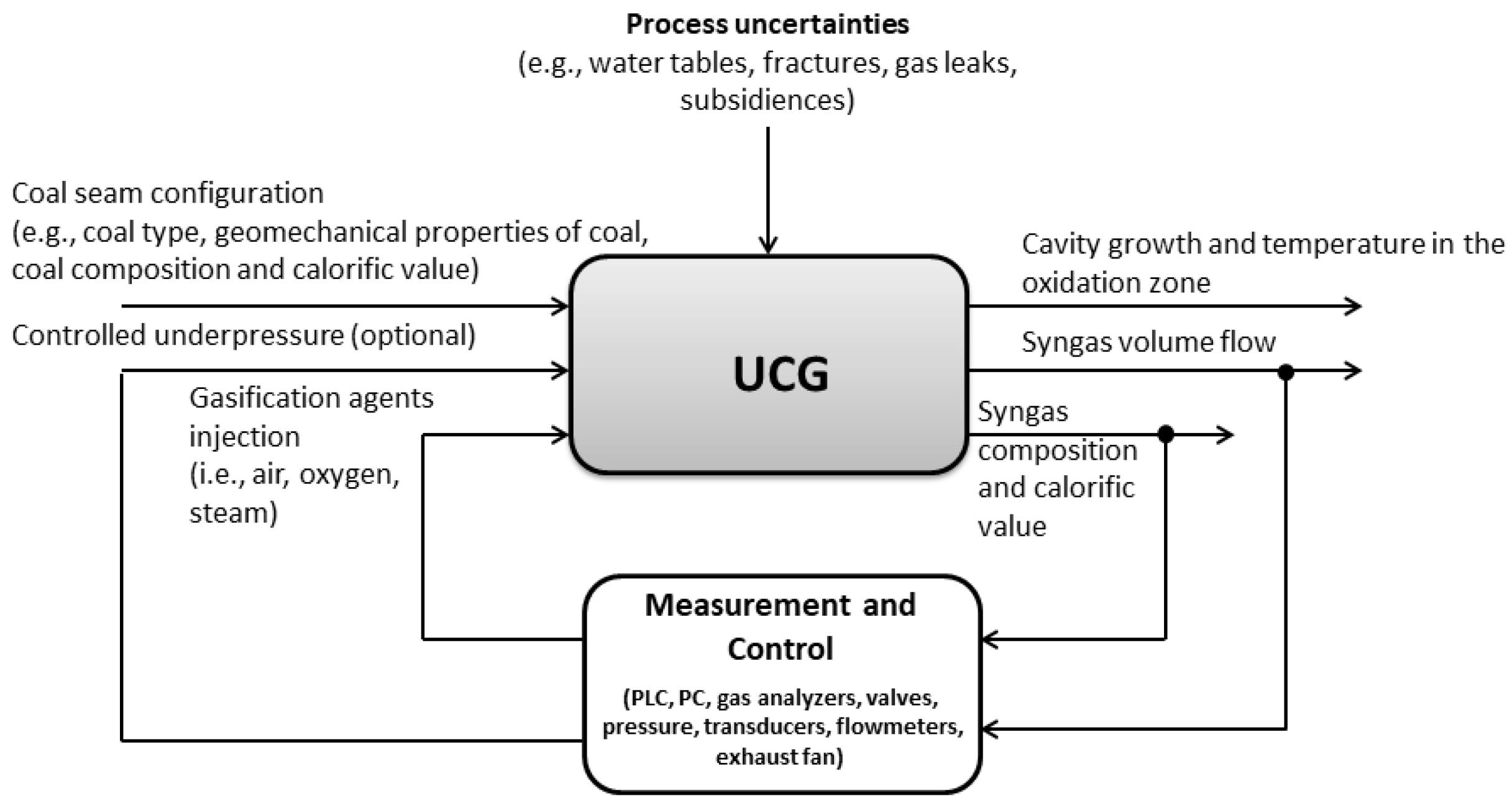
1.1. UCG Control

The main issue of UCG control is to produce syngas with stable calorific value. The control of UCG is a difficult task as, in UCG, there is a lack of direct control over many essential parameters.

The automated control of UCG can be bedeviled by a relatively considerable uncertainty of the controlled object (i.e., coal seam), which, unlike the industrial system, was created by nature. Partly this uncertainty can be reduced by a more detailed geological survey. However, even this does not guarantee the elimination of such uncertainty, as evidenced by long-term experience in the traditional coal mining technology. There may also be problems with the changing operating conditions of the process. For this reason, the control system should be robust and be able to adapt to changes in the process continuously.

The input flows of the gasifiers should be continuously optimized to ensure the required calorific value. An automated control system should be able to perform optimal control interventions and eliminate the human factor.

On the outlet from the georeactor, there is an effort to optimize suction pressure (i.e., under pressure) or directly the exhaust fan power (e.g., revolutions). The under pressure and overpressure control of UCG on the stabilization level were investigated in [25].

Kačur and Kostúr [25] have investigated the utilization of adaptive PI control to stabilize the temperature in the oxidization zone, measured by a thermocouple, with the regulated airflow and stabilization of measured oxygen concentration in syngas by regulated exhaust fan power. The adaptation of discrete controllers aimed to cope with the uncertainties in UCG. The proposed controllers were verified on an ex situ reactor.

Within experimental research of UCG improvement, an adaptive model-predictive control (AMPC) was also tested on a regression machine-based simulation model [26].

In [26], the model based on multivariate adaptive regression splines (MARS) simulated the UCG process, and the AMPC algorithm continuously optimized the three control variables (i.e., the air flow, oxygen flow, and output under pressure) to maintain the syngas calorific value setpoint. The internal prediction model of the ARX type was continuously adapted in the MPC algorithm. The simulation results showed that AMPC could achieve a better quality of calorific value stabilization with three manipulation variables than with the use of a discrete PI controller and one manipulation variable (i.e., air flow). Unfortunately, applications of MPC on industry hardware can be complicated, due to complex matrix calculations and quadratic programming [26].

Another connection of learning methods with predictive control of gasification can be found in [27]. In this work, adaptive predictive control of oxygen concentration in syngas without using a model was proposed.

Another research of automated UCG control was based on a continual adaptation of two regression models to maintain syngas calorific value [28].

This approach was also tested on an ex situ UCG reactor. Several criteria were proposed for the adaptation of regression parameters, e.g., the measure based on the desired range of the calorific value and underground temperature. The proposed models calculate optimal air flow and oxygen flow injected to the georeactor to increase or maintain the syngas calorific value during UCG operation. The regression modes were adapted by continually measured process data and the least square method. The proposed control approach has shown exciting results and demonstrated the possibility of its application on devices of industrial automation, or as a supporting algorithm for the monitoring system [28].

Another approach for estimating an optimal amount of gasification agents based on thermodynamical model was proposed in [29].

The optimization goal in [29] was to find the optimal amount of oxidizers at a known thermodynamic temperature. Optimization problems were solved by a modified gradient method for the defined weight of coal. The aim of the thermodynamics model was based on input data of UCG processes to calculate the composition of syngas at different temperatures. Based on thermodynamics, the system will be in a state of equilibrium if overall Gibson energy is at a minimal. The optimization task was solved using the method of the Lagrange multipliers [30,31].

Wei and Liu [32] have proposed a new data-based iterative optimal learning control scheme for discrete-time nonlinear systems, using the iterative adaptive dynamic programming (ADP) approach, and apply this proposed scheme to solve a coal gasification optimal tracking control problem. The neural network was used to approximate the system model using the input-state-output data of the system, and the optimal tracking control problem was transformed into a two-person zero-sum optimal regulation control problem. An iterative ADP algorithm was then established to obtain the optimal control law where the approximation errors in each iteration were considered [32].

Much research work to developing UCG advanced control has been completed by Uppal et al. [33,34].

In [34], the nonlinear time-domain UCG model was used in a closed-loop configuration with a sliding mode controller (SMC). The controller can find optimal input of the model as the molar flow rate of inlet gas (i.e., a mixture of air and steam) to keep the calorific value at the desired value in the presence of external disturbance (i.e., water influx from the surrounding aquifers). Recently, a one dimensional (1-D) packed bed model of UCG was proposed, which can be used in a closed-loop configuration with a robust controller to maintain a desired heating value of the exit gas mixture by manipulating the flow rate of injected gases. The solution of the model showed that the heating value of the exit gas is sensitive to the flow rate of inlet gases. Therefore, a robust control strategy can be employed to maintain the desired heating value in the presence of disturbances and model uncertainties by manipulating the flow rate [33,35,36,37,38].

1.2. Model-Free Control

Model-free control does not rely on any mathematical model of the controlled system. The control algorithm uses only online measurements from the real system. Model-free control can adapt to a regulated system and deal with any uncertainty in the system, as it does not rely on any specific model. One of the best-known approaches to system management without a model is extremum seeking control [39,40,41,42].

This is a model-free optimization method that was initially proposed to control train systems [43]. The main goal of such a control system is to seek an extremum, i.e., maximize or minimize a given objective function, without closed-form knowledge of the function or its gradient. In the literature, many results from the application of extremum-seeking algorithms can be found, especially after the appearance of a consistent convergence analysis in [44].

To understanding extremum seeking methods, the following general dynamics of the system can be defined:

$$\dot{x}=f\left(x,u\right),$$

(1)

where $x \in {ℝ}^n$ is the state of the system, $u \in ℝ$ is the scalar control (for simplicity), and $f$: ${ℝ}^n\times ℝ\to {ℝ}^n$ is a smooth function. We then use Equation (1) to represent the model of a real system, with the control goal to optimize a given performance of the system. This performance can be as simple as a regulation of a given output of the system to a desired constant value, or a more involved output tracking of the desired time-varying trajectory, etc. Let us now model this desired performance as a smooth function $\left(x, u\right)$: ${ℝ}^n\times ℝ\to ℝ$, which can be simply denoted as $J\left(u\right)$, as the state vector $x$ is driven by $u$.

Indeed, one of the simplest ways to maximize $J$ is to use a gradient-based extremum seeking control as follows:

$$\dot{u}=h\frac{dJ}{du}.$$

(2)

Another well-known approach to seeking extremes is the so-called extremes seeking based on perturbations. The control algorithm uses the perturbation signal to examine the control space, and sets the manipulation variables toward the local optimum by implicitly monitoring the gradient update. These types of extremum search algorithms have been thoroughly analyzed, for example, in [41,44,45,46].

The following well-known model-free control method is the co-called reinforcement learning algorithm [47,48,49,50,51,52,53].

In this method, the control algorithm tests random control actions, monitors system responses, and gradually creates a system’s predictive model. This approach to control belongs to the machine learning class. The algorithm continuously learns how to map system states to action interventions so that the objective function is maximized. The control algorithm creates a database of the best action interventions using trial and error [54].

In this work, a model-free optimal control design is presented, which continuously searches for local extremes of syngas calorific value using perturbation signals. The UCG represents numerous chemical processes, which complex model would be complicated. In this study, the UCG was considered a black-box system with known inputs and outputs (see Figure 2). Utilization of an ex situ reactor and the physical model of coal seam enables us to verify a UCG control system in lab-scale without environmental impact. The black-box approach and model-free control enable us to process control without the need to model internal processes. The controlled system, i.e., UCG georeactor, has known inputs and outputs. After ignition of the coal seam, the syngas production depends on injected oxidizers (i.e., gasification agents) and regulated under pressure.

In the following sections, the UCG ex situ reactor and the proposal of model-free optimal control of UCG are described. The aim was to design a model-free control algorithm that could be implemented on industrial hardware (e.g., PLC) or SCADA software. By introducing perturbations on the controlled system, it is possible to continuously optimize the manipulation variables to maximize the calorific value of the syngas produced. The algorithm should only work with measurable inputs (i.e., airflow or oxygen flow) and measurable outputs (i.e., syngas composition and calorific value). Verification of the control system was performed on an ex situ reactor where the influence of UCG uncertainties (e.g., fractures, surface subsidies, gas leaks, and water tables, etc.) on syngas production was not analyzed at this stage of the research.

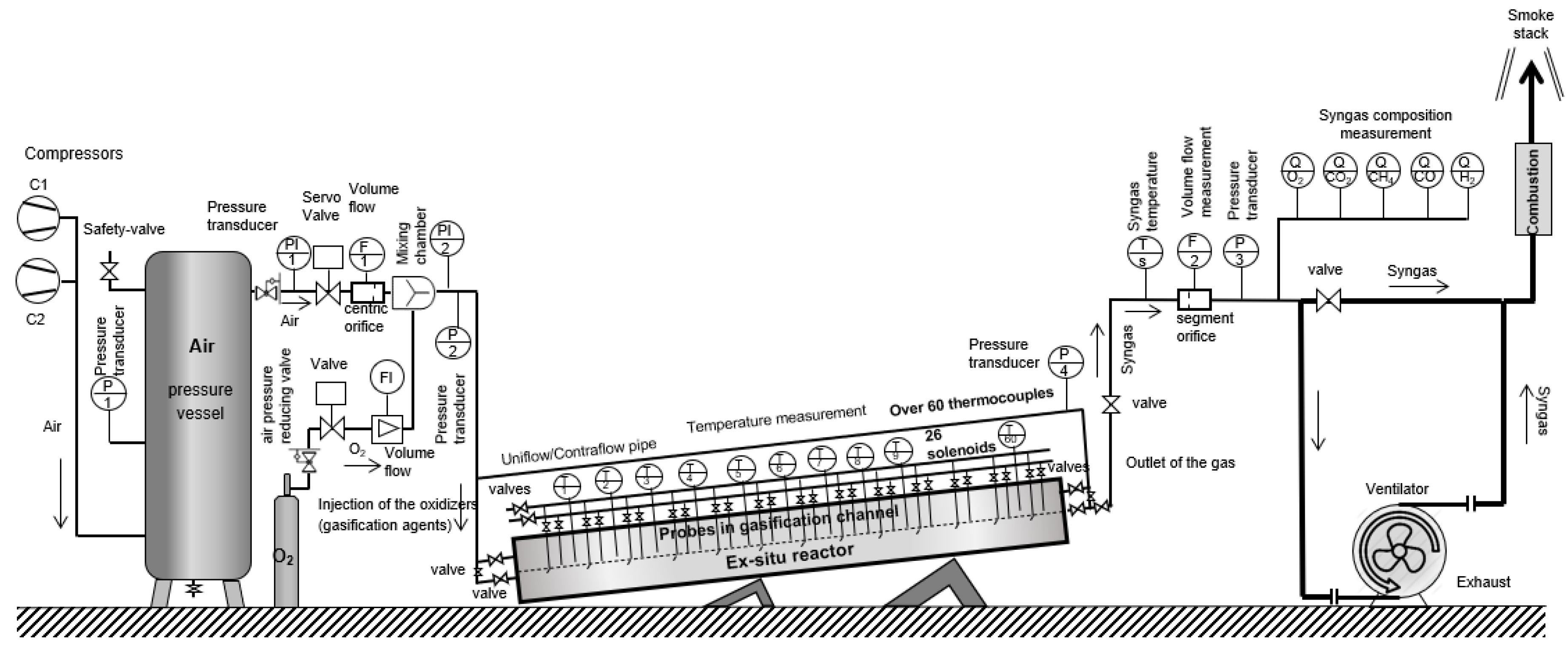
2. Experimental UCG in Ex Situ Reactor

Much research work in UCG has been performed on ex situ reactors (e.g., [6,29,55,56,57,58]). Using the ex situ reactors, the influence of various oxidants on the calorific value of syngas, the movement of the combustion front, reverse combustion, and the modeling of the temperature field was investigated. Ex situ reactors with the bedded coal represent physical models of the real coal seam. The coal storage, as well as the reactor design, meet the conditions of geometric similarity.

To test advanced control methods (i.e., adaptive and optimal), the experimental gasification equipment with a UCG ex situ reactor was constructed (see the scheme of equipment in Figure 3 and ex situ reactor in Figure 4a). A ramp with sampling points for gas analysis was constructed in the middle of the ex situ reactor. Coal was bedded longitudinally on both sides of the reactor or only on the right half.

The ex situ reactor allowed the bedding of connected blocks of coal. The coal seam model was created from glued coal blocks (see Figure 4b). For experiments, the lignite from the mine Cigeľ was used. This mine belongs to Upper Nitra coal Basin in Slovakia. During the gasification, the fired coal and layers of coal from roof stone stroke down into the formed space (see Figure 4c). After gasification, there was ash in the reactor and a partly gasified coal (see Figure 4d).

Along with the coal seam model, the gasification channel was created. This channel was created as a gap between blocks or drilled as a borehole to coal blocks. The bedded coal was isolated by a mixture of sand and water glass. The outer isolation was ensured by the sibral.

As gasification agents, atmospheric air and technical oxygen were used. They were injected into the reactor from the pressure vessels. Two compressors produced the pressure air, and pressure oxygen was delivered from the oxygen plant.

For the measurement and control, several devices were used. Figure 5 shows devices essential for the control system verification. The volume flows of gasification agents were regulated by the servo-valve and reduction valves (see Figure 5a). Pressure transducers measured the pressure of gasification agents (see Figure 5b). The volume flows of air and syngas were measured using the flow meter diaphragms and the differential pressure transducers (see Figure 5c,h). A vortex flowmeter measured the volume flow of oxygen (see Figure 5i). The mixture of air and oxygen was created in the mixing chamber. The stationary analyzers measured the composition of syngas at the output from the ex situ reactor. Using two analyzers (i.e., Madur CMS–7 and ABB Caldos (see Figure 5d)), gas concentrations as carbon monoxide (CO₂), carbon dioxide (CO), oxygen (O₂), hydrogen (H₂), and methane (CH₄) were continually measured.

The syngas calorific value was calculated from the measured gases according to the following equations:

$$H=126.4{\phi }_{\mathrm{CO}}+107.6{\phi }_{{\mathrm{H}}_2}+358.0{\phi }_{{\mathrm{CH}}_4},$$

(3)

where $H$ is the syngas calorific or heating value (KJ/m³) and ${\phi }_i$ is the volume fraction of the $i$-th fuel component in percentages.

The outlet under pressure was controlled by the power of the industry fan and frequency converter (see Figure 5e,f). The produced syngas was burned in the combustion chamber or exhausted by the smoke stack.

All devices were connected to PLC (see Figure 5g). The detailed specifications of all devices used in experimental UCG can be found in [25].

The automated control system can simultaneously perform several cyclic tasks, which provide the following operations:

• control of air pressure by two compressors;
• stabilization of airflow through servo valve;
• stabilization of temperature in the oxidizing zone;
• stabilization of the O₂ concentration in syngas.

On the pipes were placed pressure transducers. The construction of an ex situ reactor enables measurement of the pressures and syngas composition, along with the physical model of the coal seam.

The temperatures in the coal, gasification channel, and isolating overburden were measured by thermocouples of K type (up to 1300 °C). All devices for the measurement and control were connected to PLC (B & R X20: Eggelsberg, Austria) that was placed along with a frequency changer to the instrumental box (i.e., switchboard).

The control algorithms (i.e., stabilization and optimal control) were implemented on PLC as cyclic tasks. The control interventions, controllers’ setup, or monitoring of the gasification process variables were ensured by the SCADA system created in Promotic [2,20,25,26,28,55].

Table 1. Coal composition analysis (r = received, d = dry, daf = dry ash-free, and a = analytical) [25].

Parameter	Value
Total Moisture $W_t^r$ (%)	22.25
Ash $A^d$ (%)	26.33
Volatiles $V^{daf}$ (%)	60.39
Carbon $C^{daf}$ (%)	64.79
Hydrogen $H^{daf}$ (%)	5.59
Nitrogen $N^{daf}$ (%)	1.04
Calorific value $Q_i^{daf}$ (MJ/kg)	24.94
Calorific value $Q_i^d$ (MJ/kg)	18.37
Calorific value $Q_i^r$ (MJ/kg)	13.74
Ash $A^r$ (%)	20.47
Carbon $C^r$ (%)	37.11
Hydrogen $H^r$ (%)	3.20
Nitrogen $N^r$(%)	0.59
CaO (%)	1.12
MgO (%)	0.62
SiO2 (%)	12.10
Al2O3 (%)	5.26
Fe2O3 (%)	2.89
Na2O (%)	0.14
P2O5 (%)	0.02
TiO2 (%)	0.17
K2O	0.55
Volatiles $V^r$ (%)	34.59
Analytical Moisture $W^a$ (%)	9.56
Total Sulphur $S_t^r$ (%)	1.93
Sulphate Sulphur $S_S^r$ (%)	0.01
Pyritic Sulphur $S_P^r$ (%)	1.35
Organic Sulphur $S_O^r$ (%)	0.57
Oxygen $Q^{daf}$ (%)	26.34
Oxygen $Q^d$ (%)	19.4

presents the results of the coal composition analysis performed in a certified laboratory. It can be seen from the table that this is coal with higher moisture.

Within the research, the permeability of the coal sample was also analyzed using a pressure permeameter. The amount of gas forced through the sample was measured with a wet gas meter. In the pressure of 1 MPa and flow 0.000011722 m³·s⁻¹, the permeability coefficient had the value of $K$ = 2.37911 × 10⁻¹⁴ m² [59].

3. UCG Optimal Control Based on Dynamic Optimization

An optimal control algorithm finds the optimal values of control variables (i.e., manipulation variables) to achieve a certain optimality criterion (e.g., maximum profit, minimum cost, maximum calorific value, the maximum volume of produced syngas, etc.). There are two types of automatic optimization [60]:

• Optimization with the mathematical model of the process;
• Optimization without the mathematical model of the process (i.e., the system is considered as the “black-box”).

In the first case, a mathematical description of the process in the control computer is encoded. With this description, the optimal values of control variables, which are transferred to the local automatic control systems, are found. These controllers’ role is to maintain the setpoint of control variables, but the system properties change during the time. Capturing the time variability in the mathematical model is probably impossible. The mathematical model consists of a wide range of parameters determined by experimental knowledge about the system’s behavior.

In the second case, the optimal mode can be found via “experiment” on the observed object. In the controlled process, perturbations through the control variables are artificially created and, based on the analysis of results, are gradually improving the operating mode of equipment. The nonlinear programming methods are the most commonly used to find the optimal mode where the model is the physical object itself. The advantage of the first approach is that it involves a relatively simple calculation and setting of optimal conditions. The advantage of the second approach is that there is no required mathematical model of the process.

The disadvantage of the first approach is that obtaining a good model requires substantial theoretical and experimental efforts. The drawback of the second procedure is a break in the continual work of equipment.

To formulate optimization problems in general, so that it covers all possible cases, is very difficult. What follows is the formulation, which is quite near to the general formulation.

The definition of an optimization problem from a mathematical term is essentially a setup of set $\mathrm{D}\in ℝ$, and a function of multiple variables $J\left(u_1,u_2,\dots ,u_n\right)$, respectively $J\left(\overline{u}\right)\in ℝ$. Then, looking such $J\left({\overline{u}}^{opt}\right)$ so as ${\overline{u}}^{opt}\in \mathrm{D}$, $J\left({\overline{u}}^{opt}\right)\ge J\left(\overline{u}\right)$ (i.e., maximization) for all $\overline{u}\in \mathrm{D}$ was fulfilled. The set of $\mathrm{D}$ is often called an area created by limitations.

In terms of proposal of the optimal control system, the following approaches can be applied:

• Optimal control systems with feedback;
• Optimal control systems with feed-forward;
• Combined optimal control systems.

In this paper, to realize the optimal control of UCG, the optimal feedback control was proposed. The proposal is based on a static optimization method that was adapted to the dynamic process of UCG. The optimization method continually seeks local extremes of the objective function and optimizes manipulation variables. The advantage of this system is that it does not need the process model. In this case, the optimal control is achieved directly by the experimental way, where the model is a controlled object. Process behavior is performed in an iterative way so that the criterion of optimality according to an optimization algorithm was fulfilled. The first successful trial with optimal feedback control of UCG without model was reported in [42]. The optimal control system was based on direct extremum seeking of carbon monoxide concentration in syngas and gasification agent optimization. When formulating optimal control problems, it is desirable to know the optimized vector, optimality criterion, constraints, and have chosen a suitable optimization method.

3.1. Optimized Vector

Optimized vector (4) consists of variables that can be changed to obtain extremum of optimality criterion, which optimize these parameters. For optimization of the gasification process, this vector consists of three manipulation variables, with which we can dynamically influence the process.

$$\overline{u}=\left(\begin{array}{c}{u}_1\\ u_2\\ u_3\end{array}\right),$$

(4)

where $u_1$ is the servo valve opening adjusted by digital pulses. By changing the servo valve opening, the change of airflow is reached (m³/h). The airflow is the primary operating variable in experimental UCG. Although the airflow can be stabilized by PI controller, for more straightforward implementation and verification of the proposed control algorithm, we decided not to use cascade connection. Variable $u_2$ represents the oxygen flow added to the oxidation mixture (m³/h). It is the value of the desired flow adjusted directly by the servo valve. The third manipulation variable, $u_3$, is an exhaust fan motor power frequency (Hz). The change of this variable changes the fan’s revolutions, and subsequently, the suction pressure (Pa) at the outlet is affected.

3.2. Optimimality Criterion

The gasification control can be performed optimally under the chosen optimality criterion respecting restrictive conditions. Optimality systems generate optimal control, which depends on the selected optimality criterion. This criterion may be technical or economic nature. For optimal control, the gasification process can be used the following criterion of optimality:

An optimality criterion that represents the maximum calorific value of syngas was defined. The criterion was defined as functional in the form:

$$J=\underset{{\tau }_1}{\overset{{\tau }_2}{{\displaystyle \int }}}H\left(\tau \right)d\tau \to MAX$$

(5)

where $H\left(\tau \right)$ is the calorific value of the syngas in time $\tau$ (MJ/m³), and constants ${\tau }_1$ and ${\tau }_2$ are the times of the start and the end of the analyzed section (s), respectively.

Considering that the boundaries ${\tau }_1$, ${\tau }_1$ in previous integral are fixed values, and time section ${\tau }_2-{\tau }_1$ is the constant, this functional is unsuitable for practical solutions. For the realization of the optimal control system, it is preferable to use the functional in the following form:

$$J=\frac{1}{{\tau }_2-{\tau }_1}\underset{{\tau }_1}{\overset{{\tau }_2}{{\displaystyle \int }}}H\left(\tau \right)d\tau \to MAX.$$

(6)

This criterion expresses the maximal calorific value on average during optimal process control.

3.3. Constraints

In formulating the optimal control problem, consideration of limitations resulting from the process is required. These are constraints and requirements on the input and output process variables, which must not be exceeded. In technological processes, such restrictions may result either from technological requirements or the equipment’s design parameters, in which technological process occurs. For optimal control of the gasification process, which is performed on a laboratory gasifier, the following constraints can be defined:

• For the control variables, the constraints are defined as the following:

  $$u_j^{Min}\le u_j\le u_j^{Max}; \left(j=1, 2, 3\right)$$

  (7)

  where $u_1^{Max}$, $u_1^{Min}$ is the maximum and minimum of allowable servo valve opening (%, pulses) or airflow (m³/h), respectively, $u_2^{Max}$, $u_2^{Min}$ is the maximum and minimum of allowable oxygen flow (m³/h), respectively, and $u_3^{Max}$, $u_3^{Min}$ represent the maximum and minimum of allowable exhaust fan power frequency (Hz), or boundaries for controlled under pressure (Pa) on the outlet from the ex situ reactor, respectively;
• If the concentration of oxygen in the syngas is too high, it means that input is set up to a high flow of oxygen or a higher amount of oxidant is blown. High oxygen concentration at the outlet leads to a surplus of oxygen in the gasification process. It is reflected in a reduced calorific value. An ideal situation occurs when the oxygen concentration on the outlet is maintained at 0%. Given the above remarks, we can define a limit on the concentration of oxygen $\left({\phi }_{{\mathrm{O}}_2}\right)$ in the following form:

  $${\phi }_{{\mathrm{O}}_2}^{Min}\le {\phi }_{{\mathrm{O}}_2}\le {\phi }_{{\mathrm{O}}_2}^{Max},$$

  (8)

  where ${\phi }_{{\mathrm{O}}_2}^{Max}$ is the maximal permitted concentration of O₂ in syngas (%), and ${\phi }_{{\mathrm{O}}_2}^{Min}$ is the minimal permitted concentration of O₂ in syngas (%).

3.4. Optimization Method

In this paper, the simple gradient optimization method with constraints is proposed to be applied for the model-free optimal control of UCG. It is an iterative method, based on the last point approximation looking for another point in which the objective function’s value is nearer to the extreme. The speed of convergence of this method is quite good at greater distances from the extreme, and approaching the extreme, the rate of convergence decreases. This approach is suitable for multidimensional optimization problems and belongs to a group of methods called point–direction–step. Applications of gradient methods for solving a specific problem of optimal control can be found in [61,62].

The control algorithm aims to maintain the extreme (i.e., maximum) of the objective function in each control step. The research was aimed to maximize syngas calorific value, as this variable is the most critical indicator of UCG. Replacing the integral in Equation (6) by the operator of the summation, a discrete form of the objective function can be obtained:

$$J_k\left(\overline{u}\right)\approx \frac{1}{n}{\displaystyle \sum }_{i=1}^n{H}_j·∆{\tau }_j\to MAX,$$

(9)

where $J_k\left(\overline{u}\right)$ is the value of the objective function in the step $k$ (MJ/m³), $k$ is the index of the control period $T_{0,opt}$ of the optimal control algorithm, $\overline{u}$ is the vector of the manipulation variables, which are optimized by optimal control algorithm, $H$ is the calorific value of syngas (MJ/m³), $j$ is the index of the sampling period $T_{0,stab}$ on the stabilization level, $∆{\tau }_j$ is the value of $T_{0,opt}$ in the $j$–th step of the sampling, and n is the number of the samples in the buffer.

Equation (9) represents a nonlinear function that will be maximized. This task can be solved by a nonlinear optimization method with constraints.

Assuming that $∆{\tau }_j=1$ for $j=1, 2,\dots , n$ substituting into Equation (9), then the equation for calculation of the average calorific value is the following:

$$H_k{\left(\overline{u}\right)}^{average}=\frac{1}{n}{\displaystyle \sum }_{i=1}^n{H}_j,$$

(10)

where $H_k{\left(\overline{u}\right)}^{average}$ is the average calorific value (MJ/m³) of the syngas in the step k, and $H_j$ is the $j$–th calorific value in the buffer (MJ/m³).

The average calorific value of the produced gas during the period $T_{0,opt}$ is in the algorithm of optimal control calculated as a moving average of the samples recorded with a period $T_{0,stab}$. For calculation of the moving average, a FIFO buffer was used [63]. This buffer contains a historical record of the calorific value. The time length of this record is determined by the buffer size n and the sampling period $T_{0,stab}$.

Components of the vector $\overline{u}$ are continually optimized by optimal control algorithm to gradually achieve extremes of the objective function $J\left(\overline{u}\right)$. The control system sets a new opening of the servo valve according to the value of the parameter $u_1$, the desired flow of the oxygen by the parameter $u_2$, and the new frequency of changer according to the parameter $u_3$. Concerning the principle of the gradient method for maximizing the objective function, the following equation is calculated iteratively [62,64]:

$${\overline{u}}^{i+1}={\overline{u}}^i+h·\nabla J\left({\overline{u}}^i\right),$$

(11)

where ${\overline{u}}^{i+1}$ is the vector of optimized control variables in step $i+1$, ${\overline{u}}^i$ is the vector of the optimized variables in the step $i$, and $h$ is an iterative constant (step), which is chosen in such a way that the values ${\overline{u}}^{i+1}$ do not distort conditions of the existence of functions $J\left(\overline{u}\right)$, also that was true (maximizing) $J\left({\overline{u}}^{i+1}\right)>J\left({\overline{u}}^i\right)$ and, at the same time, ensure appropriate convergence of the method. Step $h$ is reduced only if the value of the objective function does not grow. Each variable of vector ${\overline{u}}^i$ can have custom parameter $h$. Then, the vector $\overline{h}={\left(h_1, h_2,h_3\right)}^T$ can be defined; $\nabla J\left({\overline{u}}^i\right)$ is the gradient of the objective function expressed as the column vector of partial differentials of the objective function according to variables $u_1^i$, $u_2^i$, $u_3^i$.

Optimization starts with the initial vector ${\overline{u}}^0={\left(u_1^0, u_2^0, u_3^0\right)}^T$. In the next step, the control history is perturbed, and the partial derivatives are calculated on each iteration. This straightforward control adjustment scheme derives the control perturbation for the ($i+1$)st iteration from the control gradient computed on the $i$-th iteration [62].

The gradient of the objective function contains the following components:

$$\nabla J\left({\overline{u}}^i\right)={\left(\frac{\partial J}{\partial u_1^i},\frac{\partial J}{\partial u_2^i},\frac{\partial J}{\partial u_3^i}\right)}^T.$$

(12)

For the approximation of gradients $\frac{\partial J}{\partial u_1^i},\frac{\partial J}{\partial u_2^i},$ and $\frac{\partial J}{\partial u_3^i}$, the finite difference method can be used. Using a forward approximation, the following equations can be obtained:

$$\begin{array}{c}\frac{\partial J}{\partial u_1^i}\cong \frac{∆J}{∆u_1^i}=\frac{J\left(u_1^i+∆u_1, u_2^i, u_3^i\right) - J\left({\overline{u}}^i\right)}{∆u_1}\\ \frac{\partial J}{\partial u_2^i}\cong \frac{∆J}{∆u_2^i}=\frac{J\left(u_1^i, u_2^i+∆u_2, u_3^i\right) - J\left({\overline{u}}^i\right)}{∆u_2}\\ \frac{\partial J}{\partial u_3^i}\cong \frac{∆J}{∆u_3^i}=\frac{J\left(u_1^i, u_2^i, u_3^i+∆u_3\right) - J\left({\overline{u}}^i\right)}{∆u_3}\end{array}$$

(13)

where $∆u_j$ is the elemental change of the manipulation variable $u_j$, $\left(j=1, 2, 3\right)$.

For the application of the gradient method, the parameters $∆u_1$, $∆u_2$, and $∆u_3$ are chosen so that the change of the parameter $u_j$ by value $∆u_j$, ($j$ = 1, 2, 3) causes a change in the value of the objective function. The objective function’s value enters into the optimal control algorithm only from the steady state of the process. Each subsequent step of the optimal control algorithm is performed only if the following condition is fulfilled:

$$\underset{j=1\dots n}{\max }\left\{\frac{\left|H_k{\left(\overline{u}\right)}^{average}-H_j\right|}{H_k{\left(\overline{u}\right)}^{average}}\right\}<{\epsilon }_{max}$$

(14)

where $H_k{\left(\overline{u}\right)}^{average}$ is the average syngas calorific value of the syngas in step $k$, $H_j$ is the $j$–th calorific value in a FIFO buffer (MJ/m³), ${\epsilon }_{max}$ is the maximum allowable deviation from the arithmetic average (%), and parameter $n$ is the number of samples in the FIFO buffer.

Alternatively, the test of steady state can be performed by calculating standard deviation according to the equation

$$\frac{1}{n}\sqrt{{\displaystyle \sum }_{k=1}^n{\left(H_k{\left(\overline{u}\right)}^{average}-H_j\right)}^2}<s_{max},$$

(15)

where parameter $s_{max}$ represents the maximum allowable value of the standard deviation.

The choosing constant ${\epsilon }_{max}$ is based on the analysis of the calorific value record. There was analysis of the settling time of the calorific value and the ability to stabilize. At each step of the record, the left-hand side of the Equation (14) was evaluated. Figure 6 shows the calorific value behavior during the experiment and the relative error of the arithmetic average as the value on the left side of the Equation (14). Calorific value is changed in carrying out different control interventions (e.g., change the servo valve position, increase oxygen flow, or change the power frequency of the exhaust fan). The graphical analysis follows that the calorific value can be considered steady when the relative deviation is not more than 25%.

When testing the algorithm, the buffer keeps a historical record of the samples from the last 30 min. It is time that corresponds to the approximate stabilization time of the calorific value. Detection of the steady state of the calorific value by evaluating condition (14) should be verified not only at each step $k$, which is performed with the period $T_{0,opt}$, but also continually in every step of the calorific value stabilization ($T_{0,stab}$). Recorded behavior of the stabilization error can serve in the analysis of the algorithm activity. If the condition (14) is fulfilled, the Boolean variable (i.e., flag) Steady in the algorithm is set to the logical value True. The buffer size and the update period can be arbitrarily set on the control panel in the monitoring system.

For the automated control of UCG, the gradient method was adapted to experimental gasification equipment and possibilities of the ex situ reactor. The algorithm flow chart is shown in Figure 7. The proposed algorithm represents one of the possible variants of gradient method application for the dynamic process. The algorithm was programmed as two cyclic tasks implemented to PLC Steps of the algorithm are performed with the period $T_{0,opt}$, and this period can be arbitrarily set from the environment of the monitoring system. During testing, in the optimal control algorithm, the period $T_{0,opt}$ was set to 900 s (i.e., 15 min).

The first cyclical task worked with period $T_{0,opt}$ and ensured the implementation of each step of the algorithm, depending on the state given by flag Steady. The objective function’s current value (in the algorithm labeled as $J$) also enters the first cyclic task.

The second cyclical task worked with the sampling period $T_{0,stab}$, detecting the stabilization of the calorific value and setting the flag Steady. When testing the optimal control algorithm, the period $T_{0,stab}$ was set to 1 min. The algorithm was also tested with $T_{0,stab}$ set to 30 and 15 s. At the same time, I second cyclic task ensures updating variable $J$, containing the current value of the objective function calculated according to Equation (9).

The proposed algorithm can optimize the three manipulation variables during the UCG and seek local extremes of the objective function, i.e., maximization of syngas calorific value. The algorithm uses perturbations to explore the control space, and steers the manipulation variables toward their local optimum by following a gradient update. The algorithm continuously seeks optimal manipulation variables to set the operating parameters as the airflow, the flow of additional oxygen, and the under pressure at the outlet. By automatic setup of the manipulation variables, the human factor is eliminated when deciding on action interventions to increase the syngas calorific value.

Considering a defined constraint (7), the following conditions must be evaluated in the algorithm:

$$\mathrm{If} u_j^{i+1}>u_j^{Max} \mathrm{then} u_j^{i+1}=u_j^{Max}; \mathrm{if} u_j^{i+1}<u_j^{Min} \mathrm{then} u_j^{i+1}=u_j^{Min} \mathrm{for} j=1,2,3.$$

As the proposed algorithm can set the various value of the oxygen flow rate, which in some cases can cause a state with a high excess of oxygen, the algorithm takes into account the constraint (8) and evaluates the following condition:

$$\mathrm{If} {\phi }_{{\mathrm{O}}_2}>{\phi }_{{\mathrm{O}}_2}^{Max} \mathrm{then} \frac{\partial J\left({\overline{u}}^i\right)}{\partial u_2^i}=0$$

where ${\phi }_{{\mathrm{O}}_2}$ is the currently measured concentration of O₂ in syngas and parameter ${\phi }_{{\mathrm{O}}_2}^{Max}$ represents the maximum allowed concentration of O₂ in syngas. When testing the algorithm, the value of the parameter ${\phi }_{{\mathrm{O}}_2}^{Max}$ was set to 10%.

Initialization of the algorithm requires a correctly chosen value of the optimization parameter $h$. The improperly selected value of this parameter can cause unexpected behavior of optimization. When the optimization is in progress, the following condition must also evaluate:

$$\mathrm{If} J\left({\overline{u}}^i\right)>J\left({\overline{u}}^{i+1}\right) \mathrm{then} h=h/2 \mathrm{until} h\le h^{Min}.$$

If $h\le h^{Min}$, or max division of $h$ exceeds, then it is necessary to determine the new initial vector $\overline{u}$, constant $h$, and re-solve the optimization task (i.e., restart and re-initiation).

4. Results

Four tests of the optimal control algorithm were performed within the experimental gasification on an ex situ reactor. The individual tests differed in the number of optimized manipulation variables and the duration. In all tests, the algorithm continuously introduced perturbations to calculate the gradients according to the Equation (13). The control algorithm optimized the manipulation variables to continuously maximize the calorific value. The algorithm worked with online mean calorific value data, which it recorded in the FIFO buffer to calculate the value of the objective function (9) within the period of optimal control $T_{0,opt}$. The algorithm was implemented on a PLC, which provided online measurement and change in manipulation variables. Changes in manipulation variables were made only when the steady state calorific value of syngas was indicated according to Equation (14). The optimal control algorithm was programmed as a cyclic task, i.e., a program implemented to PLC in Automation Basic Language. Figure 8 shows the connection diagram of the proposed UCG optimal control.

In the first experiment, the optimal control algorithm, which was tasked to maximize the calorific value and optimize two variables, was verified. Two manipulating variables, i.e., $u_1$—servo valve opening that adjusts the flow of injected air—and $u_3$—frequency of changer, that sets the exhaust fan power to effect under pressure at the outlet from the generator)—were optimized. An objective function was chosen according to Equation (9). The calorific value was entered into the algorithm as the average from the last 30 min. Within this period, the relative deviation was continuously evaluated from the arithmetic average by Equation (14). The maximum allowable relative deviation from the arithmetic average was set to 25%.

The behavior of the algorithm is shown in Figure 9. The figure shows an optimized servo valve opening to digital pulses and corresponding airflow, exhaust fan motor frequency to regulate exhausting under pressure, and behavior of calorific value with discrete values of the objective function sampled by $T_{0,opt}$. The figure also shows an improvement of the objective function concerning the value from the previous optimization step. The figure shows the application of perturbations to manipulation variables and the refinement of the parameter $h$.

The algorithm started with an initial value of objective function 2.17 MJ/m³ and, after 730 min of operation, achieved an increase to 7.4 MJ/m³. Then, calorific value only decreased, and the algorithm failed to increase it. The decrease in the calorific value was caused by low temperatures in the oxidizing zone (i.e., the temperature was less than 1000 °C). As the optimal control was deactivated after 17 h, a manual temperature increase had to be performed with the oxygen.

In another test of optimal control with optimization of two manipulation variables, the calorific value was increased from 0.95 to 2.1 MJ/m³ (see 1025 min) (see Figure 10). The test lasted more than 9 h and, during this time, was restarted twice. The automatic restart was carried out as the algorithm failed to increase the calorific value, even after several divisions of the parameter $h$.

Furthermore, an algorithm of optimal control with optimization of three variables was tested: $u_1$—servo valve opening, which adjusts the flow of injected air–$u_2$–oxygen flow—and $u_3$—frequency of changer, which sets the exhaust fan power. Each control variable had set its parameter $h$ (i.e., $h_1$ for $u_1$, $h_2$ for $u_2$, and $h_3$ for $u_3$). The behavior of the algorithm activity is displayed in Figure 11. The figure shows three manipulation variables, volume flow of injected air, and the supplementary oxygen. The figure also indicates the behavior of calorific value with discrete values of the objective function, and improvement of the objective function concerning its value from the previous optimization step. The optimal control algorithm started at an initial calorific value of 4.4 MJ/m³. During its activity for the short term, there was an increase in the calorific value to more than 9.5 MJ/m³ (101 and 611 min). The algorithm ran a total of 10 h. During this time, it was automatically restarted twice as the dividing parameter $h$, in the case of unsuccessful optimization, did not bring an increase in calorific value.

In the fourth test of optimal control, three parameters were also optimized, and the calorific value of syngas was maximized. Figure 12 shows the graph presentation of the optimization activity. The algorithm ran a total of 10 h, and the calorific value increased from an initial 4.4 to 8 MJ/m³. This result was reached by gradually reducing the airflow, increasing the flow of oxygen, and reducing exhaust fan power. The automatic restart of the algorithm was not activated during the test.

Detailed analysis showed that the maximum permissible value of the relative deviation from the arithmetic average could also be set to a lower value for the algorithm’s improvement, e.g., 10%. Smaller maximum tolerance would be extended, waiting for a stable calorific value, and extending the algorithm’s test. All four tests of the algorithm favorably affect the gasification process. In any case, the calorific value was, in the short term, increased, opening the way for further improvement and testing of the algorithm.

A summary view of the configuration of individual tests and the achieved results is shown in

Table 2. Configuration of experiments and summary of results.

Test	Duration (min)	Optimized Variables	Optimization Steps	Maximum Temperature (°C)	Average Temperature (°C)	Initial Calorific Value (MJ/m3)	Average Calorific Value (MJ/m3)	Maximum Calorific Value (MJ/m3)	Final Calorific Value (MJ/m3)
#1	1100	$u_1, u_3$	4	1050	878	2.17	4.3	8.1	7.4
#2	1150	$u_1, u_3$	5	956	815	0.95	2.1	5.5	2.1
#3	650	$u_1, u_2, u_3$	5	1194	938	4.4	4.8	14.2	9.7
#4	650	$u_1, u_2, u_3$	6	1182	1054	4.4	5.1	8.5	8.0

. The UCG experiments in which the proposed control algorithm was tested differed in time duration, number of optimized manipulation variables, and achieved temperatures in the oxidation zone. The table shows that the best results, i.e., the highest calorific values, were acquired by optimizing all three manipulation variables. A higher average temperature was also obtained in these tests. The algorithm calculates manipulation variables to ensure optimal flows gasification agents so that the content of the heating components was the greatest. This aim can be achieved only at higher temperatures above 1000 °C.

Optimization of supplemental oxygen injection has significantly improved gasification. On the other hand, gasification with oxygen can be more expensive.

5. Discussion

Optimal control based on the gradient method’s application in the four tests ensured an increase in the calorific value. The algorithm uses perturbations to explore the control space, and steers the manipulation variable toward its local optimum by following a gradient update. Thus, the advantage of the proposed solution is that no model is needed to calculate optimal manipulation variables. However, on the other hand, the proposed control needs the continual work of equipment, and finding optimal control can be relatively time consuming. The proposed algorithm was implemented on PLC and on the SCADA system.

Three manipulation variables were optimized during experiments, i.e., airflow, oxygen flow, and exhaust fan power on the outlet. These variables enable control of the behavior of the UCG. When oxygen was used as an additional oxidant, the higher temperature in the oxidation zone and syngas’ calorific value were recorded (i.e., 938–1054 °C, 4.8–5.1 MJ/m³). There was also recorded a short-term highest calorific value of 14.2 MJ/m³ in gasification with oxygen. When only air (i.e., combination of overpressure and under pressure system) was used as the sole oxidant, the average coal temperature and calorific value of the syngas were lower (i.e., 815–878 °C, 2.1–4.3 MJ/m³). The highest calorific value of 8.1 MJ/m³ was recorded during gasification with air.

Other algorithms for continuous extreme search have also been experimentally tested at UCG, and they are compared with the proposed algorithm in this paper.

Kostúr and Kačur [42] proposed an extremal controller algorithm that continuously maximized CO concentration in the syngas. The discrete extremal controller algorithm optimized only one manipulation variable, which stabilized the airflow by the PI controller. When testing the control algorithm, the CO concentration in the syngas increased by 17 vol.% (from 15 to 31%), which resulted in an increase in the calorific value of the syngas by 5 MJ/m³ (from 12 to 15 MJ/m³).

Kačur et al. [28] also tested optimal control with an adaptive regression model. The online adaptation of the regression model was based on the least-squares method, and the selected criterion was based on the calorific value of the syngas. The syngas calorific value was successfully maintained from 3 to 10 MJ/m³ during the experiment. However, this algorithm was more computationally complex and implemented within the SCADA system. In both cases, UCG control tests were performed on the same type of coal and the same ex situ reactor as used in this work.

Despite the complexity of the control system, the implemented system remains open to further improvement. It is necessary to look for such a solution so that the calorific value of syngas is sustainable in the long run. For further research in laboratory conditions, it is necessary to test the optimal control algorithm for another criterion, e.g., maximizing the temperature in the oxidation zone and maximizing economic profit or CO concentration in the produced gas.

6. Conclusions

Underground coal gasification has a range of potential benefits. The process is safer and more energy-efficient than the conventional combination of coal mining and surface combustion. At present, UCG is blindly controlled, and various automated control methods are being tested experimentally.

In laboratory conditions, the technology of UCG was investigated on an ex situ reactor with a coal seam model to find a suitable control strategy. This paper solved the problem of model-free optimal control of underground coal gasification of UCG. The proposed algorithm was based on a simple gradient method that optimizes by experimental way of operating variables.

The novelty and originality of the proposed solution of UCG control rests on a model-free approach. This approach of automated UCG control to maximize calorific value has not been investigated to date. Most of the research in the world focuses on the model-based stabilization of calorific value and mathematical modeling of UCG processes. However, research is lacking in improving the direct automated control of the UCG process that is often controlled only blindly. Furthermore, the high complexity of model-based control complicates the implementation of control on automation hardware (e.g., due to the calculation of matrices or quadratic programming). The advantage of the proposed control is the low computational complexity and the possibility of implementation on industrial hardware.

The proposed control algorithm has been implemented on a PLC; it does not require a process model, and only online measured process data are needed. The proposed algorithm, in four tests, was able to increase the calorific value by optimizing the manipulation variables. Better algorithm performance, i.e., higher syngas calorific value, was achieved by optimizing three manipulation variables, i.e., when additional oxygen flow was optimized. By optimizing the manipulation variables, the calorific value of the syngas was increased by 5 MJ/m³, both in gasification with air and additional oxygen. However, in gasification with additional oxygen, higher average calorific values (i.e., 5.1 MJ/m³) were achieved. When gasifying with air (overpressure and under pressure), the highest average calorific value obtained was 4.3 MJ/m³. Gasification with air showed a lower average temperature in the oxidation zone (878 °C) than gasification with additional oxygen (1054 °C).

Although the control system has only been tested on an experimental ex situ gasifier with minor modifications, it can also be tested on an in situ gasifier operation. Proposed control can eliminate the human factor when deciding on actions to intervene in the UCG process (i.e., correct setting of control parameters) when maintaining the maximum calorific value is necessary.

References

- Perkins, G. Mathematical Modelling of Underground Coal Gasification, Academic Dissertation; University of New South Wales, Faculty of Science and Engineering: Sydney, NSW, Australia, 2005. [Google Scholar]
- Kačur, J.; Durdán, M.; Laciak, M.; Flegner, P. Impact analysis of the oxidant in the process of underground coal gasification. Measurement 2014, 51, 147–155. [Google Scholar] [CrossRef]
- Chandellea, V.; Lia, T.K.; Ledenta, P.; Patignya, J.; Henqueta, H.; Kowola, K.; Massona, G.; Mostadea, M. Belgo-German Experiment on Underground Gasification Demonstration Project; Technical Report; Commission of the European Communities: Brussels, Belgium, 1989; ISBN 92-825-9673-7. [Google Scholar]
- Creedy, D.P.; Garner, K.; Holloway, S.; Jones, N.; Ren, T.X. Review of Underground Coal Gasification Technological Advancements; Technical Report COAL R11 DTI/Pub URN 01/1041; Department of Trade and Industry: London, UK, 2001. [Google Scholar]
- Anon. Underground Coal Gasification Program; Report ERDA 77-51/4 on Contract No. EX-76-C-01-2343, Technical Report; Booz, Allen & Hamilton, Inc.: Washington, DC, USA; US Energy Research and Development Administration: McLean, VA, USA, 1977. [Google Scholar]
- Dobbs, R.L.; Krantz, W.B. Combustion front Propagation in Underground Coal Gasification, Final Report, Work Performed under Grant No. DE-FG22-86PC90512; Technical Report; Boulder Department of Chemical Engineering, University of Colorado: Boulder, CO, USA, 1990. [Google Scholar]
- Cena, R.J.; Thorsness, C.B. Underground Coal Gasification Database; Technical Report UCID-19169; Lawrence Livermore National Laboratory, University of California: Berkeley, CA, USA, 1981. [Google Scholar]
- Gibb, A. The Underground Gasification of Coal; Sir Isaac Pitman & Sons Ltd.: London, UK, 1964. [Google Scholar]
- Gregg, D.W.; Hill, R.W.; Olness, D.U. An Overview of the Soviet Effort in Underground Coal Gasification; Technical Report UCRL-52004; Lawrence Livermore Laboratory, University of California: Berkeley, CA, USA, 1976. [Google Scholar]
- Olness, D.U. The Angrenskaya Undergroud Coal Gasification Station; Technical Report UCRL-53300; Lawrence Livermore National Laboratory, University of California: Berkeley, CA, USA, 1982. [Google Scholar]
- Anon. Underground Coal Gasification—First Trial in the Framework of a Community Collaboration: Final Summary Report; Technical Report; Underground Gasification Europe (UGE): Alcorisa, Spain, 1999. [Google Scholar]
- Boysen, J.E.; Canfield, M.T.; Covell, J.R.; Schmit, C.R. Detailed Evaluation of Process and Environmental Data from the Rocky Mountain I Underground Coal Gasification Field Test; Technical Report No. GRI-97/0331; Gas Research Institute: Chicago, IL, USA, 1998. [Google Scholar]
- Robert, G.M.M.; Oliver, L.; Spackman, L.K. Field and laboratory results from the TONO 1 (CRIP) UCG Cavity Excavation Project. WIDCO Mine Site, Centralia, Washington. Fuel Sci. Technol. Int. 1989, 7, 1059–1120. [Google Scholar]
- Walker, L.K.; Blinderman, M.S.; Brun, K. An IGCC Project at Chinchilla, Australia Based on Underground Coal Gasification UCG. In Proceedings of the 2001 Gasification Technologies Conference, San Francisco, CA, USA, 8–10 October 2001; pp. 1–6. [Google Scholar]
- Koenen, M.; Bergen, F.; David, P. Isotope Measurements as a Proxy for Optimizing Future Hydrogen Production in Underground Coal Gasification, News in Depth. 2015. Available online: https://www.tno.nl/media/2624/information20-nid1.pdf (accessed on 26 May 2021).
- Brasseur, A.; Antenucci, D.; Bouquegneau, J.-M.; Coëme, A.; Dauby, P.; Létolle, R.; Mostade, M.; Pirlot, P.; Pirard, J.-P. Carbon stable isotope analysis as a tool for tracing temperature during the El Tremedal underground coal gasification at great depth. Fuel 2002, 81, 109–117. [Google Scholar] [CrossRef]
- Wu, J.M. Radon Distribution Under the Mine and the Application of Radon Measuring in the Monitoring of the Natural Fire Zone. Ph.D. Thesis, Shanxi Institute of Mining and Technology, Taiyuan, China, 1994. [Google Scholar]
- Wu, H.S. The Measuring Methods of Radon and Its Application; Nuclear Energy Press: Beijing, China, 1995. [Google Scholar]
- Wu, H.S.; Bai, Y.S.; Lin, Y.F.; Chang, G.L. The Action of Relay Transmission of Radon Migration. Chin. J. Geophys. 1997, 40, 136–142. [Google Scholar]
- Kačur, J.; Durdán, M.; Laciak, M.; Flegner, P. A Comparative Study of Data-Driven Modeling Methods for Soft-Sensing in Underground Coal Gasification. Acta Polytech. 2019, 59, 322–351. [Google Scholar] [CrossRef] [Green Version]
- Ge, Z.; Sun, Q.; Zhang, N. Changes in surface roughness of sandstone after heating and cooling cycles. Arab. J. Geosci. 2020, 13. [Google Scholar] [CrossRef]
- Schrauf, T.W.; Evans, D.D. Laboratory studies of gas flow through a single natural fracture. Water Resour. Res. 1986, 22, 1038–1050. [Google Scholar] [CrossRef]
- Chen, Z.; Narayan, S.P.; Yang, Z.; Rahman, S.S. An experimental investigation of hydraulic behavior of fractures and joints in granitic rock. Int. J. Rock Mech. Min. Sci. 2000, 37, 1061–1071. [Google Scholar] [CrossRef]
- Ge, Y.; Kulatilake, P.H.S.W.; Tang, H.; Xiong, C. Investigation of natural rock joint roughness. Comput. Geotech. 2014, 55, 290–305. [Google Scholar] [CrossRef]
- Kačur, J.; Kostúr, K. Approaches to the Gas Control in UCG. Acta Polytech. 2017, 57, 182–200. [Google Scholar] [CrossRef] [Green Version]
- Kačur, J.; Flegner, P.; Durdán, M.; Laciak, M. Model Predictive Control of UCG: An Experiment and Simulation Study. Inf. Technol. Control 2019, 48, 557–578. [Google Scholar] [CrossRef]
- Hou, Z.; Liu, S.; Yin, C. Local Learning-based Model-Free Adaptive Predictive Control for Adjustment of Oxygen Concentration in Syngas Manufacturing Industry. IET Control Theory Appl. 2016, 10, 1384–1394. [Google Scholar] [CrossRef]
- Kačur, J.; Laciak, M.; Durdán, M.; Flegner, P. Application of multivariate adaptive regression in soft-sensing and control of UCG. Int. J. Model. Identif. Control 2019, 33, 246–260. [Google Scholar] [CrossRef]
- Laciak, M.; Ráškayová, D. The using of thermodynamic model for the optimal setting of input parameters in the UCG process. In Proceedings of the ICCC 2016 17th International Carpathian Control Conference, High Tatras, Slovakia, 29 May–1 June 2016; pp. 418–423. [Google Scholar] [CrossRef]
- Laciak, M.; Kostúr, K.; Durdán, M.; Kačur, J.; Flegner, P. The analysis of the underground coal gasification in experimental equipment. Energy 2016, 114, 332–343. [Google Scholar] [CrossRef] [Green Version]
- Laciak, M.; Kačur, J.; Kostúr, K. The verification of thermodynamic model for UCG process. In Proceedings of the ICCC 2016 17th International Carpathian Control Conference, High Tatras, Slovakia, 29 May–1 June 2016; pp. 424–428. [Google Scholar] [CrossRef]
- Wei, Q.; Liu, D. Adaptive dynamic programming for optimal tracking control of unknown nonlinear systems with application to coal gasification. Trans. Autom. Sci. Eng. IEEE 2014, 11, 1020–1036. [Google Scholar] [CrossRef]
- Uppal, A.A.; Bhatti, A.I.; Aamir, E.; Samar, R.; Khan, S.A. Control oriented modeling and optimization of one dimensional packed bed model of underground coal gasification. J. Process Control 2014, 24, 269–277. [Google Scholar] [CrossRef]
- Arshad, A.; Bhatti, A.I.; Samar, R.; Ahmed, Q.; Aamir, E. Model Development of UCG and Calorific Value Maintenance via Sliding Mode Control. In Proceedings of the 2012 International Conference on Emerging Technologies, Islamabad, Pakistan, 8–9 October 2012; pp. 1–6. [Google Scholar] [CrossRef]
- Uppal, A.A.; Bhatti, A.; Aamir, E.; Samar, R.; Khan, S. Optimization and control of one dimensional packed bed model of underground coal gasification. J. Process Control 2015, 35, 11–20. [Google Scholar] [CrossRef]
- Uppal, A.A.; Alsmadi, Y.M.; Utkin, V.I.; Bhatti, A.I.; Khan, S.A. Sliding mode control of underground coal gasification energy conversion process. IEEE Trans. Control Syst. Technol. 2018, 26, 587–598. [Google Scholar] [CrossRef]
- Uppal, A.A.; Butt, S.S.; Bhatti, A.I.; Aschemann, H. Integral sliding mode control and gain-scheduled modified Utkin observer for an underground coal gasification energy conversion process. In Proceedings of the 23rd International Conference on Methods and Models in Automation and Robotics, Miedzyzdroje, Poland, 27–30 August 2018; pp. 357–362. [Google Scholar] [CrossRef]
- Uppal, A.A.; Butt, S.S.; Khan, Q.; Aschemann, H. Robust tracking of the heating value in an underground coal gasification process using dynamic integral sliding mode control and a gain-scheduled modified Utkin observer. J. Process Control 2019, 73, 113–122. [Google Scholar] [CrossRef]
- Sira Ramirez, H.; Luviano-Juárez, A.; Ramírez-Neria, M.; Zurita-Bustamante, E.W. Active Disturbance Rejection Control of Dynamic Systems; Butterworth-Heinemann an Imprint of Elsevier: Oxford, UK, 2017. [Google Scholar]
- Zhang, C.; Ordóñez, R. Extremum-Seeking Control and Applications: A Numerical Optimization-Based Approach; Springer: New York, NY, USA, 2012. [Google Scholar] [CrossRef]
- Ariyur, K.B.; Krstić, M. Real-Time Optimization by Extremum-Seeking Control; John Wiley & Sons, Inc.: New York, NY, USA, 2003. [Google Scholar] [CrossRef]
- Kostúr, K.; Kačur, J. Extremum Seeking Control of Carbon Monoxide Concentration in Underground Coal Gasification. IFAC PapersOnLine 2017, 50, 13772–13777. [Google Scholar] [CrossRef]
- Leblanc, M. Sur lélectrification des chemins de fer au moyen de courants alternatifs de fréquence élevée. Rev. Générale Lelectricité 1922, 12, 275–277. [Google Scholar]
- Krstić, M.; Wang, H.H. Stability of extremum seeking feedback for general nonlinear dynamic systems. Automatica 2000, 36, 595–601. [Google Scholar] [CrossRef]
- Tan, Y.; Nesic, D.; Mareels, I. On the dither choice in extremum seeking control. Automatica 2008, 44, 1446–1450. [Google Scholar] [CrossRef]
- Rotea, M.A. Analysis of multivariable extremum seeking algorithms. In Proceedings of the 2000 American Control Conference ACC (IEEE Cat. No.00CH36334), Chicago, IL, USA, 28–30 June 2000; pp. 433–437. [Google Scholar] [CrossRef]
- Busoniu, L.; Babuska, R.; De Schutter, B. A Comprehensive Survey of Multiagent Reinforcement Learning. IEEE Trans. Syst. Man Cybern. Part C 2008, 38, 156–172. [Google Scholar] [CrossRef] [Green Version]
- Rao, R.P.N. Reinforcement Learning: An Introduction; Sutton, R.S., Barto, A.G., Eds.; MIT Press: Cambridge, MA, USA, 1998; 380p, ISBN 0-262-19398-1. [Google Scholar]
- Bertsekas, D.; Tsitsiklis, J. Neuro-dynamic programming: An overview. In Proceedings of the 34th IEEE Conference on Decision and Control, New Orleans, LA, USA, 13–15 December 1995; Volume 1, pp. 560–564. [Google Scholar] [CrossRef] [Green Version]
- Szepesvári, C. Algorithms for Reinforcement Learning. Synth. Lect. Artif. Intell. Mach. Learn. 2010, 4, 1–103. [Google Scholar] [CrossRef] [Green Version]
- Busoniu, L.; Babuska, R.; De Schutter, B.; Ernst, D. Reinforcement Learning and Dynamic Programming Using Function Approximators; CRC Press: Boca Raton, FL, USA, 2010. [Google Scholar] [CrossRef] [Green Version]
- Farahmand, A. Regularization in Reinforcement Learning. Ph.D. Thesis, University of Alberta, Edmonton, AB, Canada, 2011. [Google Scholar]
- Kormushev, P.; Calinon, S.; Caldwell, D.G. Robot motor skill coordination with EM-based Reinforcement Learning. In Proceedings of the 2010 IEEE/RSJ International Conference on Intelligent Robots and Systems, Taipei, Taiwan, 18–22 October 2010; pp. 3232–3237. [Google Scholar] [CrossRef] [Green Version]
- Benosman, M. Adaptive Control: An Overview. In Learning-Based Adaptive Control; Elsevier: New York, NY, USA, 2016; pp. 1–35. [Google Scholar] [CrossRef]
- Kostúr, K.; Laciak, M.; Durdán, M.; Kačur, J.; Flegner, P. Low-calorific gasification of underground coal with a higher humidity. Measurement 2015, 63, 69–80. [Google Scholar] [CrossRef]
- Wiatowski, M.; Kapusta, K.; Stańczyk, K. Efficiency assessment of underground gasification of ortho-and meta-lignite: Highpressure ex-situ experimental simulations. Fuel 2019, 236, 221–227. [Google Scholar] [CrossRef]
- Stańczyk, K.; Kapusta, K.; Wiatowski, M.; Swiadrowski, J.; Smolinski, A.; Rogut, J. Experimental simulation of hard coal underground gasification for hydrogen production. Fuel 2012, 91, 40–50. [Google Scholar] [CrossRef]
- Kapusta, K.; Wiatowski, M.; Stańczyk, K. An experimental ex-situ study of the suitability of a high moisture ortho-lignite for underground coal gasification (UCG) process. Fuel 2016, 179, 150–155. [Google Scholar] [CrossRef]
- Kačur, J.; Kostúr, K. Research Report of the Project “Underground Gasification by Thermal Decomposition No. APVV-0582-06 for Year 2008”; Technical Report; Technical University of Košice, Faculty BERG and HBP a.s. Prievidza: Košice, Slovakia, 2008. [Google Scholar]
- Hrubina, K. Optimálne Riadenie I a II; Edičné stredisko VŠT v Košiciach: Košice, Slovakia, 1987. [Google Scholar]
- Hrubina, K. Riešenie Problémov Optimálneho Riadenia, Metódami Numerickej Analýzy, Záverečná Správa o Fakultnej Výskumnej Úlohe; Technical Report; E-Fak 9 VŠT Košiciach: Košice, Slovakia, 1975. [Google Scholar]
- Stengel, R.F. Optimal Control and Estimation; Dover, Inc.: New York, NY, USA, 1994. [Google Scholar]
- Hanuš, B.; Modrlák, O.; Olehla, M. Číslicová Regulace Technologických Procesů. Algoritmy, Matematicko-Fyzikálni analýza, Identifikace, Adaptace, 1. Vydání; Vysoké Učení Technické v Brňe, VUTIUM: Brno, Czech Republic, 2000. [Google Scholar]
- Kostúr, K. Optimalizácia Procesov; Edičné stredisko TU v Košiciach: Košice, Slovakia, 1991. [Google Scholar]