Striated Tire Yaw Marks—Modeling and Validation

Abstract

Tire yaw marks deposited on the road surface carry a lot of information of paramount importance for the analysis of vehicle accidents. They can be used: (a) in a macro-scale for establishing the vehicle’s positions and orientation as well as an estimation of the vehicle’s speed at the start of yawing; (b) in a micro-scale for inferring among others things the braking or acceleration status of the wheels from the topology of the striations forming the mark. A mathematical model of how the striations will appear has been developed. The model is universal, i.e., it applies to a tire moving along any trajectory with variable curvature, and it takes into account the forces and torques which are calculated by solving a system of non-linear equations of vehicle dynamics. It was validated in the program developed by the author, in which the vehicle is represented by a 36 degree of freedom multi-body system with the TMeasy tire model. The mark-creating model shows good compliance with experimental data. It gives a deep view of the nature of striated yaw marks’ formation and can be applied in any program for the simulation of vehicle dynamics with any level of simplification.

1. Introduction

The rectified projection of tire yaw marks deposited on the road surface (often either from an orthophotomap, a point cloud or a total station survey) can be used in a macro-scale for:

• determination of subsequent vehicle positions and orientation during critical movement by matching the position of individual wheels to the corresponding marks;
• estimation of the vehicle’s speed at the start of yawing.

For the latter—assuming the vehicle was moving on a horizontal and homogeneous surface along a curve of radius $r$—the critical speed formula (CSF) is most commonly used:

$$v=\sqrt{\mu ·g·r},$$

(1)

where: µ—tire-to-roadway coefficient of friction, $r$—radius of the mark, $g$ = 9.8 m/s²—gravitational acceleration.

Although this formula may seem simplistic, it has been shown repeatedly over the years that, under certain conditions, it can be considered as a quasi-empirical critical speed method (CSM). A broad overview of such conditions has been presented among others by Brach and Brach [1]. Sledge and Marshek [2] examined some refined forms of the CSF which account for the effects of, among others, vehicle weight distribution, slip angles, cornering stiffnesses and ABS. Cannon [3] has demonstrated that effective braking causes the CSF to overestimate the speed at the start of the yaw mark and that a 50 ft. chord appears to give acceptably low effective braking-related errors (<7%) for speeds of approximately 72 km/h (45 mph) and for speeds of approximately 97 km/h (60 mph) with light to moderate braking. Cliff et al. [4] have concluded that when using the peak coefficient of friction, both the CSF and simulation over-estimated the actual speed, whereas slide coefficient of friction under-estimated them. Braking tended to increase the results. Amirault and MacInnis [5] carried out a total of 29 tests at speeds of 80 to 95 km/h. Bearing in mind non-braking and ABS braking tests, using 20 m chord measurements for the radius and the average braking coefficient of friction overestimated the measured speed by 4.1% ± 6.3% (±1σ), while using a center of gravity trajectory for the radius and the average braking coefficient of friction underestimated the measured speed by 2.0% ± 5.2% (±1σ).

Lambourn [6] conducted tests in which passenger cars were freely coasting, braking or under power when travelling in a curve at speed of 55 to 100 km/h, and proposed a procedure which makes it possible to limit the uncertainty of speed calculated from the CSF to ±10%. In [7] and [8] he concluded that his previously described CSM gives satisfactory results also in the event of light braking, heavy braking with ABS, acceleration and the operation of ESP. There was no sign of the cycling of the ABS. The yaw marks had the typical appearance, practically the same as in the case of low braking without ABS. Significantly less yaw or off-tracking were observed when compared with marks deposited with little or no braking. If the brakes were applied aggressively during the yaw, the amount of yaw would decrease. This feature—the reverse of usual yawing with the heavy non-ABS braking—is probably the result of the “select low” algorithm.

While most authors, notably Lambourn [6,7,8] and Amirault and MacInnis [5], limit their analysis to yawing with relatively low yaw rate, Cash and Crouch [9] derived a formula which accounts for a higher degree of vehicle yaw and any brake force (not only from driver input), resulting in a narrower error band than conventional CSMs. If the exact path and orientation of the collision vehicle are not readily apparent, their method allows the flexibility of considering ranges for the required values.

What distinguishes simulation methods is that they provide a deep view into the time histories of curvilinear movement parameters, including the critical speed, as well as identifying a set of data (e.g., steering angle, braking/accelerating level of particular wheels, yaw moment of inertia etc.) which enables a virtual vehicle to move along the actual tire marks.

The point of this article is the appearance of yaw marks in the micro-scale, that is from the perspective of the topology of striations forming the mark, which make it possible to infer the braking or acceleration status of the wheels (and sometimes even the steering angle of the front wheels). The yaw mark is essentially left by the entire tire footprint remaining in contact with the roadway (contact patch), but its blackness and distinctness depend on the local slip of the tread blocks relative to the road, and stress. The rule “the greater the stress, the more distinct the mark” applies both in the macro (when observing the entire yaw marks, the most pronounced are the marks of the external, loaded wheels) and in the micro scale (the most visible is the outer edge of a single yaw mark).

Yamazaki and Akasaka in their classic article [10] argue that deposition of striations is independent of the tread pattern and is caused by an in-plane bending moment that is transmitted from the roadway to the body of the tire via the tread contact patch during sharp cornering. They refer to this phenomenon as the bending buckling behavior of a steel-belted radial tire. Buckling occurs immediately in the contact patch in the presence of a large lateral reaction from the road and is specific to radial—not bias—tires. Yamazaki in [11] shows that sharp cornering turns on steel-belted radial tires often cause wavy wear along the periphery of the shoulder.

Beauchamp et al. in [12] summarize the literature concerning the yaw mark striations issue, analyze the differences in the mechanism in which striations are deposited, and discuss the relationship between tire mark striations and tire forces. They conclude that in the case of tires with pronounced shoulder blocks the striations are typically produced by these blocks whereas tires with very low pressure or without a tread pattern are more likely to deposit striations by buckling. In the absence of braking and acceleration the striation marks are parallel to the wheel rotation axis. When the brakes are applied aggressively, the striations will change to a direction more in line with the wheel trajectory but ABS prevents the tires from locking. Beauchamp et al. in [13] show examples where the striations reflect point loading of the tread shoulder blocks. In Figure 1 of their article they show a mark on which two stripes can be distinguished: lighter striations from the inside, being deposited by the tread, and darker striations from the outside, being deposited by the shoulder blocks. A scheme of formation of such a mark they demonstrate in Figure 3 of [13].

The authors of this work, in their research practice, have encountered all the types of yaw marks mentioned before—two examples are shown in Figure 1. In both cases the vehicle was yawing, but the tire mark (a) was deposited by a buckled, zero-pressure tire during a clockwise yaw, while the tire mark (b) was left by the leading shoulder blocks of the normal-pressure tire during a counter-clockwise yaw.

The article by Beauchamp et al. [13] does an excellent job of analyzing yaw mark striations from the viewpoint of its geometry and deriving equations for the calculation of longitudinal slip $s_x$ using the striation marks angle $\theta$ and the slip angle $\alpha$ see analogous formulae (9) and (11) derived in this article). It was shown that the model offers insight into the braking actions of a driver at the time the tire marks were being deposited. The usefulness of such marks for accident analysis depends obviously on their quality and clarity, which affect the uncertainty in the measurement of the geometric parameters. Beauchamp et al. in [15] explore the sensitivity and uncertainty of the $s_x$ equation. They prove that at $\alpha$ = 5°, the striations will change over 70 degrees between no braking and maximum braking, while at $\alpha$ = 85°, less than 2 degrees separate no braking and maximum braking. In the first case braking will likely be easy to distinguish; in the second, changes in striation angle from braking are unlikely to be detected.

Undoubtedly, all researchers who focus on point loading of the tread shoulder blocks as well as in-plane buckling are right in their specific areas, as in general, the appearance of a striated mark left during curvilinear motion depends on many factors, the main ones being:

• Camber angle of the wheel (which in turn depends on the suspension kinematics);
• Structure to the tire;
• Cornering, longitudinal and vertical stiffnesses of the tire (which depend among others things on tire pressure);
• Tire aspect ratio (sidewall height divided by tire width);
• Tire tread depth;
• Dynamic tire offset (pneumatic trail);
• Composition of rubber compound;
• Road surface properties; and
• Temperature in the contact patch.

However, regardless of whether the striations occur from buckling or tread blocks, their direction always follows the direction of the resultant tire velocity vector in the contact patch (called the wheel slip velocity and hereinafter referred to as $v_{IO}$). The only difference lies in the pitch of the striations, which in the case of striations created by the tread shoulder blocks gives the opportunity to estimate the longitudinal slip $s_x$ from the topology of the striations (according to the formula of Beauchamp et al. [13], see also Equations (9) to (12) in this article), while in the case of buckling does not give the same possibility because of lack of a buckling wave pitch (a momentary and unique period of the buckling wave).

An in-depth look at the mechanics of the yaw mark creation is very interesting not only as a mathematical problem, but first of all crucial from the angle of the uncertainty of vehicle accident analysis (see e.g., [16]).

2. Assumptions to the Model

For the development of a model of creating a striated tire yaw mark the following assumptions have been made:

• To describe the tired wheel–road interaction, a semi-physical, non-linear tire model TMeasy was used [17,18]. All its features, such as longitudinal and lateral forces, aligning moment, other moments resulting from the wheel kinematics, first-order dynamics for longitudinal, lateral and torsional strain, and dynamic tire offset are taken into account.
• The yaw mark creation model is universal, i.e., it applies to any curvilinear motion of a tire in lateral drift, when the wheel moves along any trajectory with variable curvature, and the wheel is subject to an unsteady force and moment as to the value and direction, calculated by solving the system of non-linear differential equations of vehicle dynamics.
• As this area is in fact the dominant one, the yaw mark will be created by the tread elements of the tire shoulder forming the outer border (during curvilinear movement of the vehicle) of the patch in contact with the road. For the yaw mark curved to the left these will be the right patch border, and for the mark curved to the right the left patch border. As the striations being deposited by the internal tread elements of the patch are usually not very clear, they have been omitted; however, if necessary, it will be easy to extend the algorithm by following the model described.
• It is possible to define any, including non-uniform, pitch of the tread shoulder blocks of the tire.
• Semi-physical tire models of class TMeasy, Magic Formula [19], HSRI [20] etc. do not describe the tire in-plane buckling, therefore this phenomenon can instead be analyzed in two ways:

  (a)

  partially, i.e., as to the tire mark course and the striations direction only; it is then sufficient to enter any pitch of the tread shoulder blocks;

  (b)

  fully, i.e., as to the tire mark course, and striations direction and pitch, if the buckling pitch in the patch is known in some other way, which can be manually entered into the program.

3. Basic Terms Concerning Movement of a Wheel in a Bend

A concise, computer-friendly vector-matrix notation has been used. The italic small letters (e.g., $v$) mean scalars, bold small letters (e.g., $v$)—vectors, and bold capital letters (e.g., $A$)—matrices. In the vector-matrix equations the Rill’s subscript notation [18] has been used:

{}

the symbol of a reference frame, e.g., the term {I} should be read “in the reference frame I”;

{I}

the ground-fixed inertial (global) reference frame with the origin at point I; the $z_I$ axis is parallel to the gravitational acceleration vector $g$ and points upward;

$r_{IO,I}$

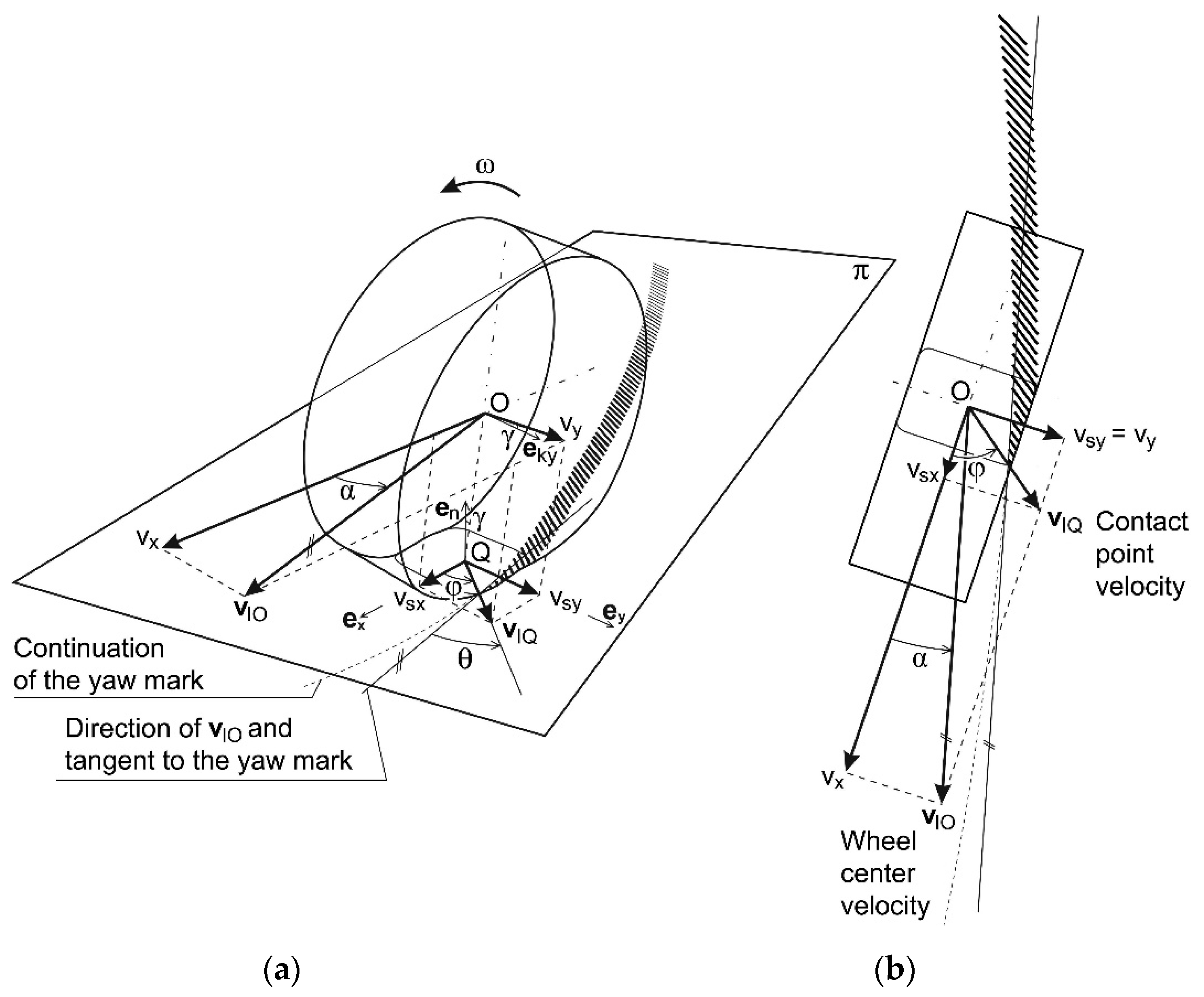
vector from point I to wheel center O; the subscript after the comma denotes the reference frame in which this vector is observed—here {I};

$v_{IO,I}$

vector of absolute velocity of wheel center O, with respect to {I}.

A characteristic point of the tire-road patch Q, which is the origin of the Cartesian coordinate system with unit vectors on its axes $e_x$, $e_y$, $e_n$ (shown in Figure 2a), is referred to as the contact point. In the TMeasy tire model, the system of forces acting on the wheel is reduced to an equivalent system of forces ($F_x, F_y$ and $F_z$) and their moments ($M_x, M_y$ and $M_z$), whose directions of action coincide with the directions of the unit vectors. The position of the rim center plane in relation to the road is determined by the position vector $r_{IO}$ and the unit vector $e_{ky}$, normal to this plane and defining the wheel rotation axis.

Camber $\gamma$ as well as cornering cause the tire to deflect laterally and to offset the contact point Q against the rim center plane by the distance $y_e$ (see Section 5.3). The road surface geometry in {I} defines the function:

$$z_s=z_s\left(x,y\right).$$

(2)

The current position of the contact point Q in the global reference frame {I} is given by the formula:

$$r_{IQ,I}=r_{IO,I}+r_{OQ,I} ,$$

(3)

where the vector $r_{OQ,I}$ can be determined by the approach given in [18] or [21].

Figure 2a depicts a diagram of a wheel in lateral slip which rolls across the plane π with angular velocity $\omega$. The following symbols have been adopted:

• $v_x$ and $v_y$—components of the wheel center velocity vector $v_{IQ}$ parallel to π, the first of which lies on the direction of the longitudinal axis of the rim, and the other is perpendicular to it;
• $\gamma$—camber angle;
• $\alpha$—wheel slip angle;
• $\omega$—wheel angular velocity about its spin axis given by the unit vector $e_{ky}$;
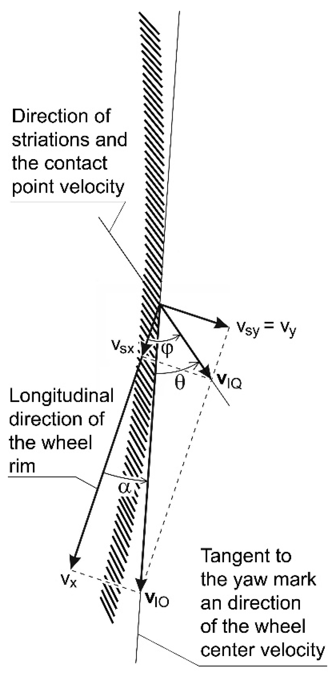
• $v_{sx}$ and $v_{sy}$—components of the absolute velocity vector of the contact point $v_{IQ}$ (wheel slip velocity); $v_{sx}$ and $v_{sy}$ are parallel to $v_x$ and $v_y$, and read:

  $$v_{sx}=v_x-r_d\omega ,$$

  (4)

  $$v_{sy}=v_y,$$

  (5)
• $r_d$—dynamic tire radius;
• $\phi$—direction of the contact point velocity $v_{IQ}$ against the longitudinal axis of the wheel (rim).

According to the ISO definition (see also Pacejka [19]), the longitudinal and lateral relative slips are:

$$s_x=-\frac{v_{sx}}{v_x}=-\frac{v_x-r_d\omega }{v_x},$$

(6)

and

$$s_y=\tan \alpha =-\frac{v_{sy}}{v_x}$$

(7)

respectively. The vectors of the contact point velocity $v_{IQ}$, the relative slip $s={\left[s_x s_y\right]}^T$ and the tangential force acting on the tire at the contact point $F={\left[F_x F_y\right]}^T$ have the same direction, and satisfy the relationship:

$$\tan \phi =\frac{v_{sy}}{v_{sx}}=\frac{s_y}{s_x}=\frac{F_y}{F_x},$$

(8)

wherein the components $F_x$ and $F_y$ are calculated according to the TMeasy (or any other) tire model.

It is easy to see that the relation (8) will also be fulfilled with other definitions of slips $s_x$ and $s_y$, because they differ only in the denominator (e.g., at Rill $r_d\left|\omega \right|$ [18] or at Mitschke $\max \left\{r_d\omega ,v_x\right\}$ [22]), which will disappear when inserted into the formula (8).

4. Wheel Velocities and Slips Versus Geometry of the Striated Tire Mark

Figure 2 shows, schematically, the process of making a striated yaw mark on the road surface with the tread shoulder blocks of a tire. The direction of the velocity vector $v_{IQ}$ is also the direction of the contact point Q displacement relative to the road and, consequently, the direction of striations deposited on the road by the tire during yaw.

Dividing the formula (7) by (8) gives:

$$s_x=\frac{\tan \alpha }{\tan \phi } ,$$

(9)

and because $s_y=\tan \alpha$, hence

$$s_y=s_x\tan \phi .$$

(10)

These relationships allow the wheel slips $s_x$ and $s_y$ to be calculated having only the striated yaw mark, as shown in Figure 3. Unlike the angle $\theta$ (representing the deviation of the striations direction from the tangent to the yaw mark, which is easy to measure on the mark), the slip and contact point velocity angles—$\alpha$ and $\phi$ respectively—are generally unknown because of the unknown orientation of the wheel relative to the mark. This difficulty applies in particular to the front wheel marks, as the steering angle of these wheels against the vehicle body is variable, and may even change over time, and are therefore impossible to determine by the yaw marks topology alone.

That is why Beauchamp et al. [13], using simple geometric relationships, derived the following formula for the slip angle:

$$\alpha =\arcsin \frac{S\sin \theta }{T}-\theta ,$$

(11)

where the distances S and T shown in Figure 4 mean:

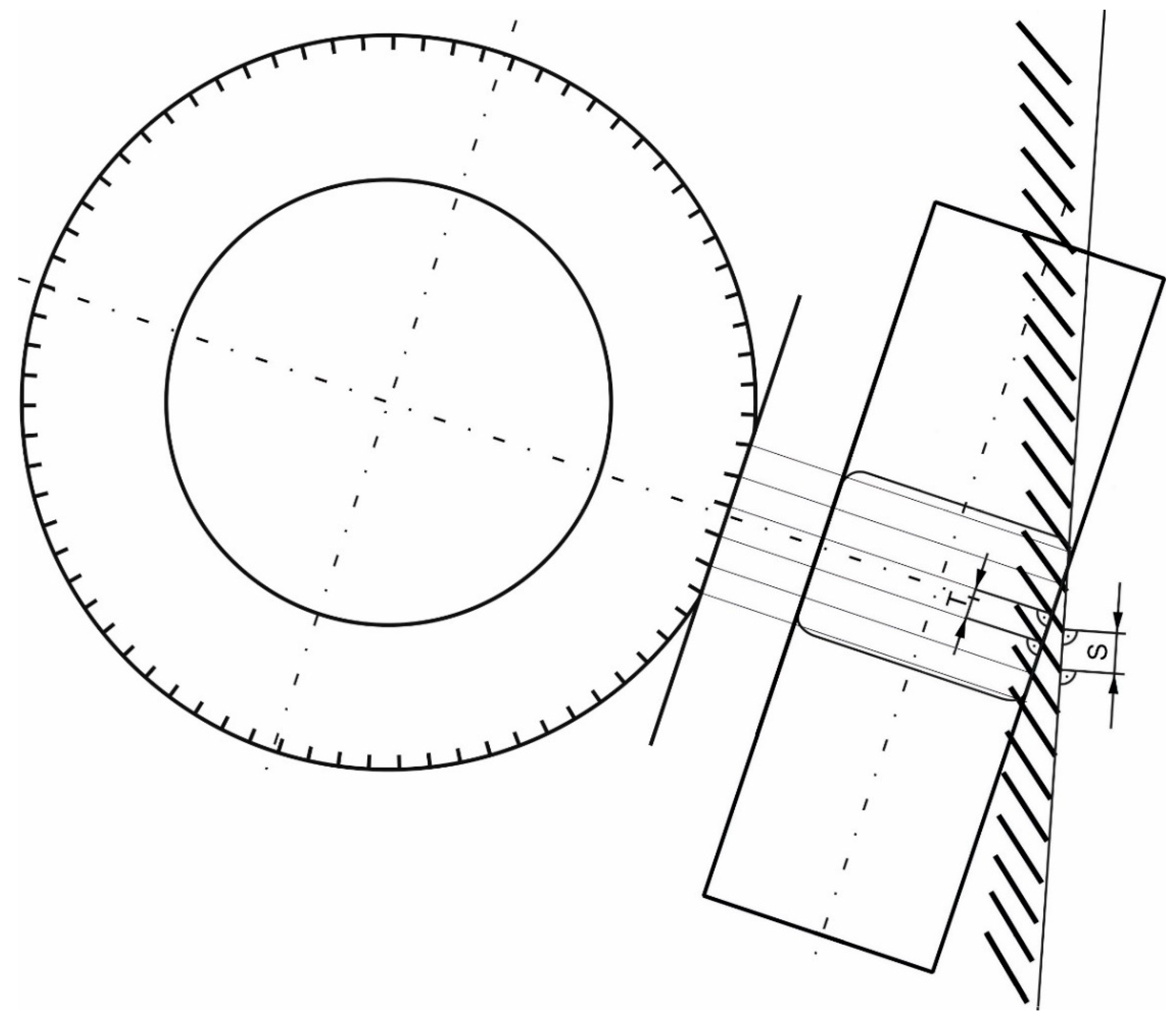
• S—the striation pitch measured along the yaw mark;
• T—the pitch of the tread shoulder blocks measured on the tire circumference.

From Figure 3 it follows that:

$$\phi =\alpha +\theta .$$

(12)

To sum up, in order to calculate the wheel slippage at a selected point of the striated yaw mark one should:

• Measure the angle $\theta$ and distance S on the mark;
• Measure the distance T at the tire shoulder;
• Calculate the angles $\alpha$ and $\phi$ from the formulae (11) and (12) respectively (note: in the case of non-steered rear wheels, when, in addition, the marks of other wheels allow one to discover successive angular positions of the vehicle by matching the corresponding wheels, the orientation of the rear wheel relative to the yaw mark is known, therefore angles $\alpha$ and $\phi$ can be measured directly on the mark—see Figure 3);
• Calculate $s_x$ and $s_y$ from formulae (9) and (10).

The uncertainty of the results of such calculations related to non-uniform pitch of the striations S (as a consequence of the uneven tread pitch T aimed at reducing the noise generated by the tire) falls within the general uncertainty of this approach and, above all, the S and T measurement uncertainty.

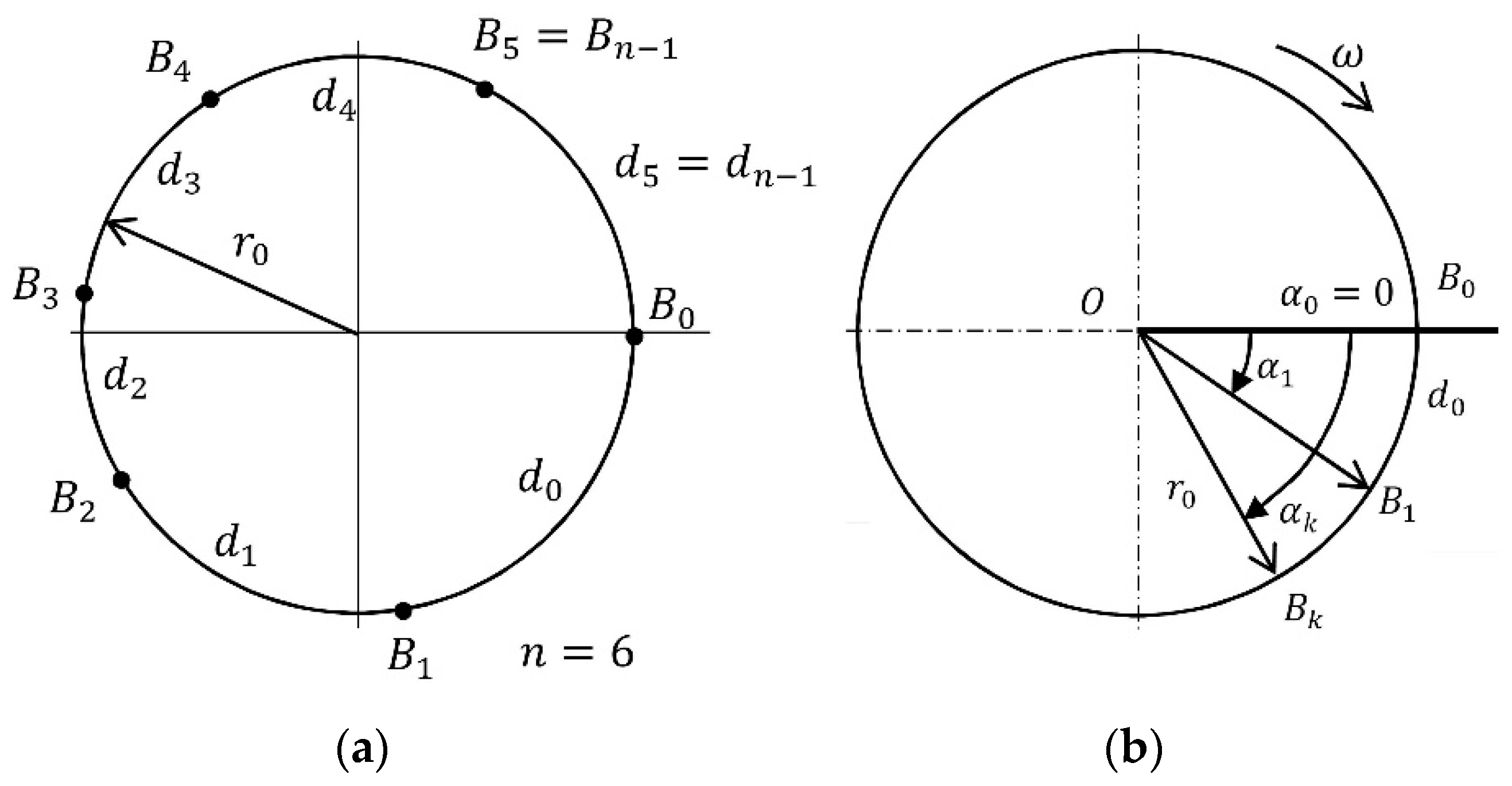
5. Model of Deposition of the Yaw Mark Striations on the Road Surface

Figure 5a shows a diagram of tread shoulder blocks pitch, where:

• $n$—number of blocks or grooves on the tread shoulder (consistently keeping to the chosen convention);
• $B_k$, $k=0,\dots ,n-1$—point indicating the $k$-th block (or groove);
• $d_k, k=0,\dots , n-1$—distances between adjacent points $B_k$ measured along an arc: with typical tires, without making a significant error, these can be measured in a straight line;

According to Figure 5a:

$$d_k=\{\begin{array}{ccc}\mathrm{distance}\mathrm{between}\mathrm{the}\mathrm{points} B_k\mathrm{and}{B}_{k+1}& \mathrm{for}& k=0,\dots , n-2\\ \mathrm{distance}\mathrm{between}\mathrm{the}\mathrm{points}{B}_k\mathrm{and}{B}_0& \mathrm{for}& k=n-1\end{array}$$

$r_0$—unloaded tire radius.

The values of parameters $d_k$ and $r_0$ are constant throughout the simulation. In general, the pitch can be defined as non-uniform ($d_k$ = constant), but in the simplest case, the program may suggest by default a uniform pitch according to the formula:

$$d_k=\frac{2\pi r_0}{n}, k=0,\dots ,n-1.$$

(13)

Let’s adopt additional symbols:

• $i$—number of simulation step;
• $t$—current simulation time;
• $h$—simulation timestep.

The following calculation algorithm, repeated in each simulation step, can be proposed.

5.1. Determining the Position of Each Point $B_k$ Relative to the Wheel-Fixed Reference Frame {O}

The origin of the wheel-fixed reference frame {O} is at the wheel center O, where the xz plane is the rim center plane and the y axis is the wheel rotation axis (with the unit vector $e_{ky}$).

This can be done in the polar coordinate system shown in Figure 5b, where point $B_k$ has coordinates $\left(r_0, {\alpha }_k\right)$. In each simulation step the angle ${\alpha }_k$ of each point is measured from the thick horizontal line, clockwise.

At the beginning of the simulation (i.e., $i=0$, $t=0$ s) point $B_0$ has the polar coordinates $\left(r_0, {\alpha }_0\right)=\left(r_0,0\right)$ and the other points $B_k$ have the coordinates $\left(r_0, {\alpha }_k\right)$, where:

$${\alpha }_k={\alpha }_k\left(t\right)={\alpha }_{k-1}+\frac{d_k}{r_0} \left[\mathrm{rad}\right], k=1,\dots ,n.$$

(14)

This formula can be applied in the function Angular_position_of_block() shown in Appendix A (Code 1), in section Code 1.

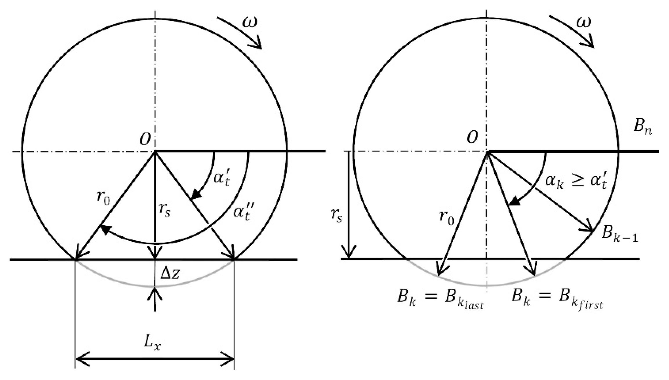
5.2. Calculation of the Characteristic Dimensions of the Contact Patch

Assuming that the tire remains in full contact with the road over the entire tread width $L_b$, and the contact patch has a rectangular shape with length $L_x$ and width $L_y$, these dimensions can be calculated using the approximation proposed by Rill in [21]:

$$L_x=L_x\left(t\right)\approx 2\sqrt{r_0\mathsf{\Delta }z}=2\sqrt{r_0\frac{F_z}{c_R}} ,$$

(15)

$$L_y=L_y\left(t\right)\approx \frac{L_b}{\cos \gamma } ,$$

(16)

where:

• $\mathsf{\Delta }z$ is the total tire deflection given by the formula:

  $$\mathsf{\Delta }z=\mathsf{\Delta }z\left(t\right)=r_0-r_s=\frac{F_z}{c_R},$$

  (17)
• $F_z=F_z\left(t\right)$—the normal reaction of the roadway to the tire at the contact point;
• $c_R=\mathrm{const}$—the radial stiffness of the tire;
• $r_s=r_s\left(t\right)$—the loaded (static) tire radius;
• $\gamma =\gamma \left(t\right)$—the tire camber angle, i.e., the inclination of the rim center plane against the roadway normal.

For example, for a tire 205/55 R16 at $F_z$ = 4700 N and the pressure $p$ = 2.5 bar, after adopting the data $c_r$ = 265000 N / m and $r_0$ = 0.317 m, one gets $L_x$ ≈ 0.15 m.

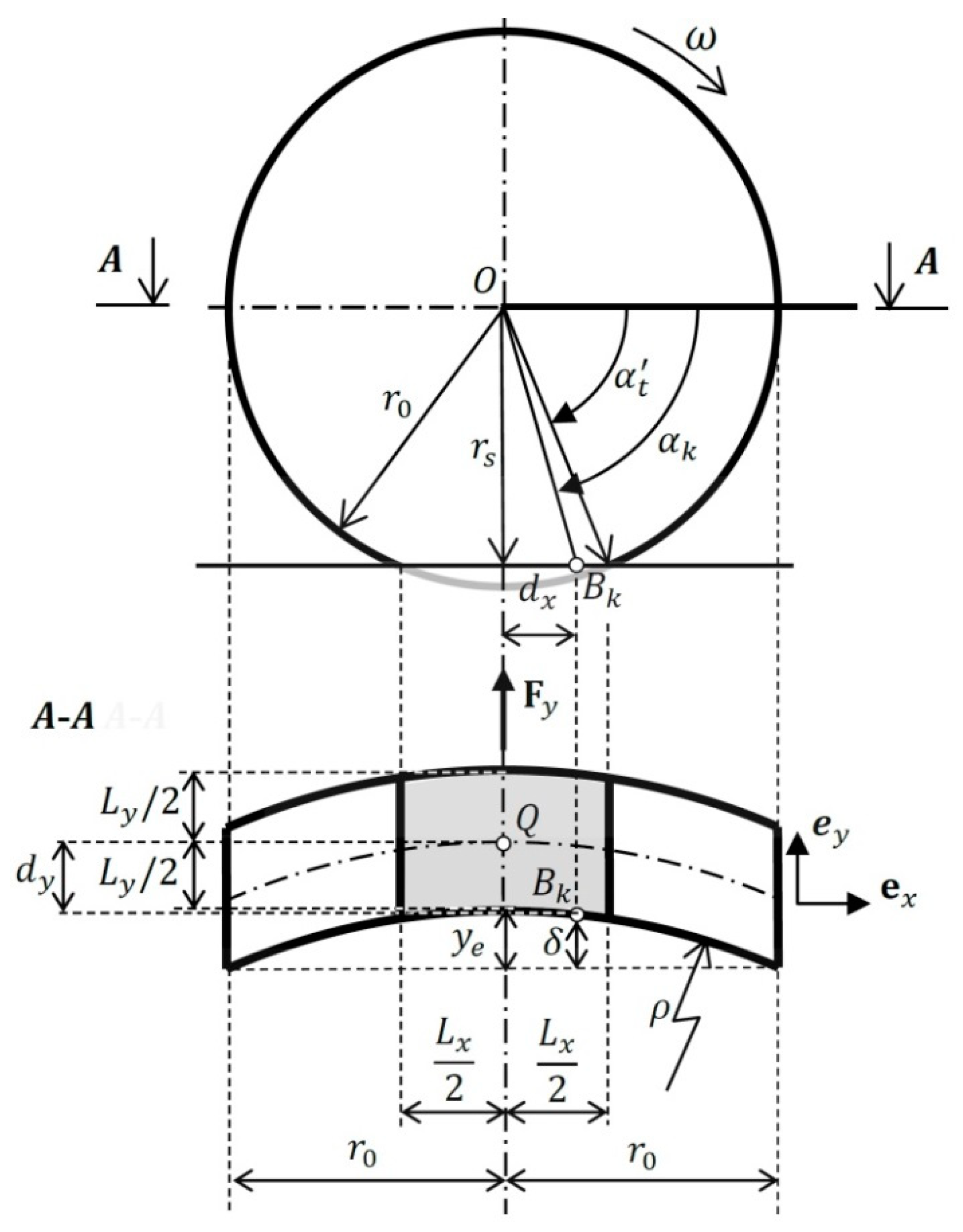
5.3. Calculating the Geometry of Striations

In a single simulation step the coordinates of the points at which the shoulder blocks contact the road should be determined. They are shown in the global Cartesian coordinate system {I}.

In reality, the deposition of a yaw mark on the road surface depends on many local or temporary factors that are difficult to discover after the accident. As the main one is a sufficiently high lateral tire force, the following formula can be used to define the condition when the yaw mark should be created in the program:

$$F_y\ge \frac{p_{\%}}{100} \mu F_z ,$$

(18)

where:

• $F_y=F_y\left(t\right)$—current lateral force acting on the tire, calculated according to the TMeasy (or any other) tire model;
• $F_z=F_z\left(t\right)$—current normal force to the roadway acting on the tire;
• $\mu$—tire-road friction coefficient; in general $\mu =\mu \left(x,y\right)$;
• $p_{\%}$—percentage of the maximum horizontal force $\mu F_z$ at which the yaw mark is to be made; by default $p_{\%}=$ 95% can be adopted.

The length of the contact patch is limited by two boundary angles ${\alpha }_t^{\prime }$ and ${\alpha }_t^{″}$ indicating the first and last point, respectively, of the tire circumference being in contact with the road (not to be confused with the point $B_k$ indicating the tread element). They are illustrated in Figure 6 and given by the formulae:

$${\alpha }_t^{\prime }=\arccos \frac{L_x}{2r_0}=\arctan \frac{2r_s}{L_x}$$

(19)

and

$${\alpha }_t^{″}=\frac{\mathsf{\pi }}{2}+\arcsin \frac{L_x}{2r_0}.$$

(20)

In order to find the indexes $k$ of all points $B_k$ in contact with the road, to begin with the indexes of the first and last contact points have to be determined using the following short algorithms.

Determining the index of the first tread block in the contact patch $k_{first}$—see Code 2 in Appendix A.

Determining the index of the last tread block in the contact patch $k_{last}$—see Code 3 in Appendix A.

Now the coordinates of the points forming the striations of the yaw mark on the road in {I} can be calculated. Figure 7 shows a simplified diagram of the lateral deflection of a tire while driving on a curvilinear track.

In fact, the deflection of the tire in the top view has a slightly more complex shape, but taking into account the assumptions made earlier, only the outer arc-shaped contour of the contact patch will be relevant (see Figure 4a,b in [10]). Thus, without making a significant error, it can be assumed that it is a fragment of a circle with a radius $\rho$ determined by chord $y_e$ and middle coordinate $2r_0$ from the formula:

$$\rho =\frac{1}{2}\left(\left|y_e\right|+\frac{r_0^2}{\left|y_e\right|}\right).$$

(21)

In Figure 7 the distances $d_x$ and $d_y$ lying on the road plane are indicated, which are distances from the tire-road contact point Q to the point $B_k$ measured along and across the wheel, respectively. The first one is:

$$d_x=\frac{r_s}{\tan {\alpha }_k }$$

(22)

and the other

$$d_y=\frac{L_y}{2}+y_e-\delta .$$

(23)

Since

$$\delta =\sqrt{{\rho }^2-d_x^2 }-\rho +y_e ,$$

(24)

hence the formula (23) takes the form:

$$d_y=\frac{L_y}{2}-\sqrt{{\rho }^2-d_x^2 }+\rho .$$

(25)

Finally, the position of the point $B_k$ is:

$$r_{I{B}_k,I}=r_{IQ,I}+d_x{e}_{x,I}-d_y{e}_{y,I} ,$$

(26)

where: $e_{x,I}, e_{y,I}$ are the unit vectors of the wheel in the point Q, shown in Figure 2a and Figure 7.

The algorithm for calculation of the vector $r_{I{B}_k,I}$ components is outlined in the section Code 4 in Appendix A.

The next step of the simulation will be:

• Incrementation of the index indicating the simulation step $i=i+1$;
• Time incrementation $t_i=t_{i-1}+h$;
• Calculation of the new angular position of the point $B_0$;

  $${\alpha }_{0_i}={\alpha }_{0_{i-1}}+{\omega }_{i}h \left[\mathrm{rad}\right],$$

  where ${\omega }_i$ is the current angular velocity of the wheel about its spin in [rad];
• Checking if the wheel has not already made a full rotation—See Code 5 in Appendix A.
• Repeating the calculations from the formula (14)—strictly from the function Angular_position_of_block() (section Code 1 in Appendix A)—to formula (26);
• Archiving the coordinates of the patch points drawing the striations.

A single striation is drawn by connecting the positions of the point $B_{k_i}$ with lines in successive, adjacent steps $i$, as long as the condition (18) is satisfied. The striated yaw mark can be being drawn as the simulation proceeds or exported at the end as a drawing file (e.g., dxf).

6. Validation and Discussion

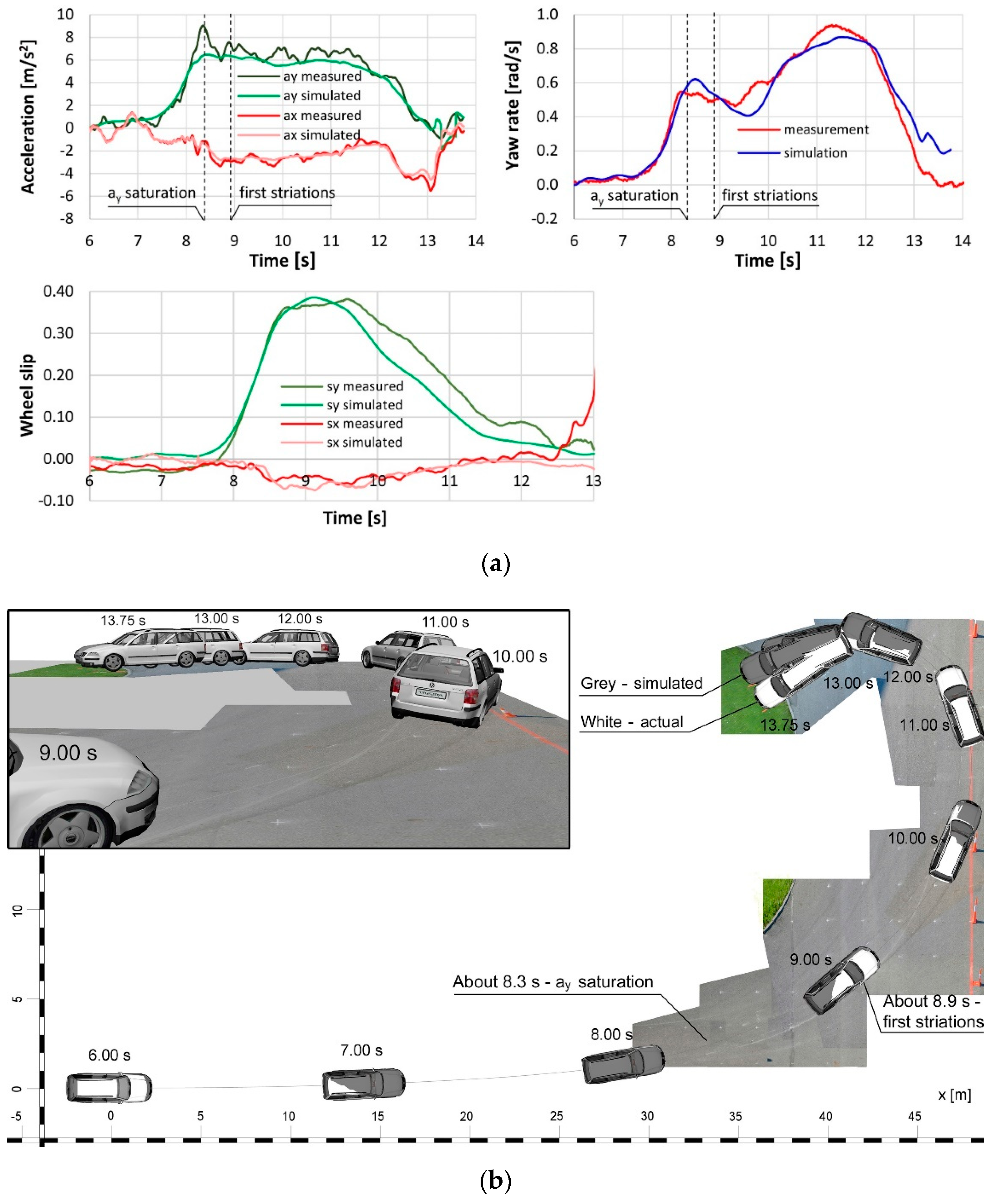
6.1. Stage 1. Measurement of Time Histories of Vehicle Motion Parameters (Actual Data)

The model was validated using the results of one of the full scale vehicle yaw tests performed as part of the Research Project No. VII/W-2014 of the Institute of Forensic Research [14]. The test vehicle was a 2003 Volkswagen Passat 2.0 TD station wagon, with Firestone FireHawk 195/65R15 91T tires with their normal inflation pressure.

Experiments were performed in the summer, on a level, horizontal and dry asphalt road surface. In the test selected for validation, having established the speed of 53 km/h in a straight line the test driver steered the vehicle hard to the left causing the tires to break the grip on the roadway and to deposit striated yaw marks.

As a result of kinematic transformations of the raw measurement data the following parameters were obtained:

• A set of kinematic data fully describing the spatial movement of the vehicle, and, first of all, time histories of three components of the CG position vector and quasi-Euler body angles (transformations—see [23]);
• Time histories of the actual longitudinal $s_x$ and lateral $s_y$ slip of the front right wheel (transformations—see Appendix of [14]).

For example, assuming the notations as in Figure 8, the absolute velocity of the wheel center O, expressed in the local, rim fixed reference frame {O}, can be calculated from the vector equation:

$$v_{IO,O}=A_{OA}{A}_{IA}^{\mathrm{T}}{v}_{IO,I}=A_{OA}\left[A_{IA}^{\mathrm{T}}{v}_{IA,I}-\left({\mathsf{\omega }}_{IA,A}\times r_{OA,A}\right)\right],$$

(27)

where:

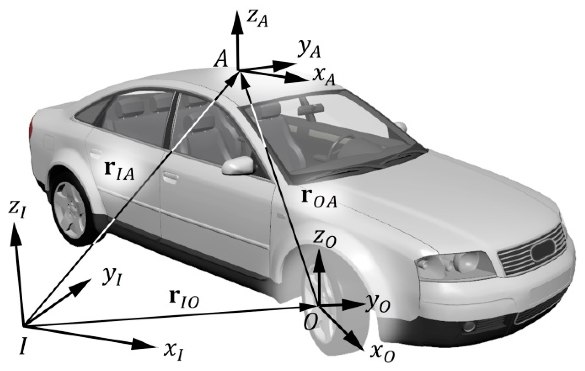
• $A_{IA}$—rotation matrix from the local, body fixed reference frame {A} to the global reference frame {I};
• $A_{OA}$—rotation matrix from from {A} to {O};
• $v_{IO,I}$—absolute velocity of the wheel center O in {I};
• $v_{IA,I}$—velocity of the GPS receiver mounting point A in {I};
• ${\mathsf{\omega }}_{IA,A}$—angular velocity of the body in {A};
• $r_{OA,A}$—position vector from point O to A in {A}.

Thus, all parameters describing the movement of the vehicle (including all points, especially wheels) in the domains of time and space are known.

6.2. Stage 2. Vehicle Movement Simulation and Its Verification

The results of the measurements described in the Stage 1 were used to verify the yaw marks creation model, which is the very core of this article. It was implemented by the author-developed multibody dynamics simulation program Model.exe, briefly outlined in the Appendix of [24]. It was assumed that the vehicle is a multibody system with 36 degrees of freedom (DoF), composed of rigid bodies connected by geometric constraints, divided into the following partial-systems: basic—body with wheel suspensions, steering and drive. The equations of motion were generated using the Jourdain’s principle. The tire forces were determined with the TMeasy model described in [17,18].

The vehicle motion was simulated, the model of which was parametrized according to the basic measurements data listed in

Table 1. Technical data of the tested Volkswagen Passat

Parameter	Value
Vehicle mass distribution on wheels:
left front	465	kg
right front	475	kg
left rear	345	kg
right rear	350	kg
Distance of CG from front axle	1.148	m
CG height	0.55	m
Wheelbase	2.703	m
Steering system ratio	16:1

. In simulation the measured time histories of the parameters shown in Figure 9 were adopted:

(a)

steering wheel angle ${\delta }_H\left(t\right)$;

(b)

external torques $M_{G1}\left(t\right)=M_{G2}\left(t\right)$ acting on the front wheels (left and right respectively) relative to their self-rotation axes.

The simulation results represented in Figure 10a,b of the time histories of various dynamic parameters, show good agreement with the actual data. In Figure 10c the simulated and actual positions and orientations of the vehicle have been compared. For as long as approximately 12 s they are almost identical, and some divergence of the CG paths occurs only at the very end of the movement. The differences may arise from the approximate torque waveform shown in Figure 9b, and partly from the simplified parametrization of the steering and drive systems and the neglected pavement unevenness.

In Figure 10a, a large discrepancy can be observed for the slip $s_x$ of the front right wheel at the end of the simulation. The relative longitudinal slip $s_x$ expressed by the formula (6) is the absolute slip (defined by the numerator) related to the speed $v_x$ of the wheel center (denominator). Although the absolute slip within the entire time range 6–13 s is small, the low speed just before the vehicle stops (12–13 s) caused a sharp and disproportionate increase in the value of the relative slip $s_x$. In other words, the reason for the sudden increase in the measured $s_x$ are low values of $v_x$ and $r_d\omega$ together with inaccuracies in the independent measurement of this parameters.

Simulation, as a theoretical process, is free of measurement flaws, hence even small numbers are precise and correlated enough that dividing them gives reasonable results. That is why at the end of the simulation, at low speeds, a disturbing difference between the measured and simulated slips $s_x$ occurred. This issue should not be overestimated.

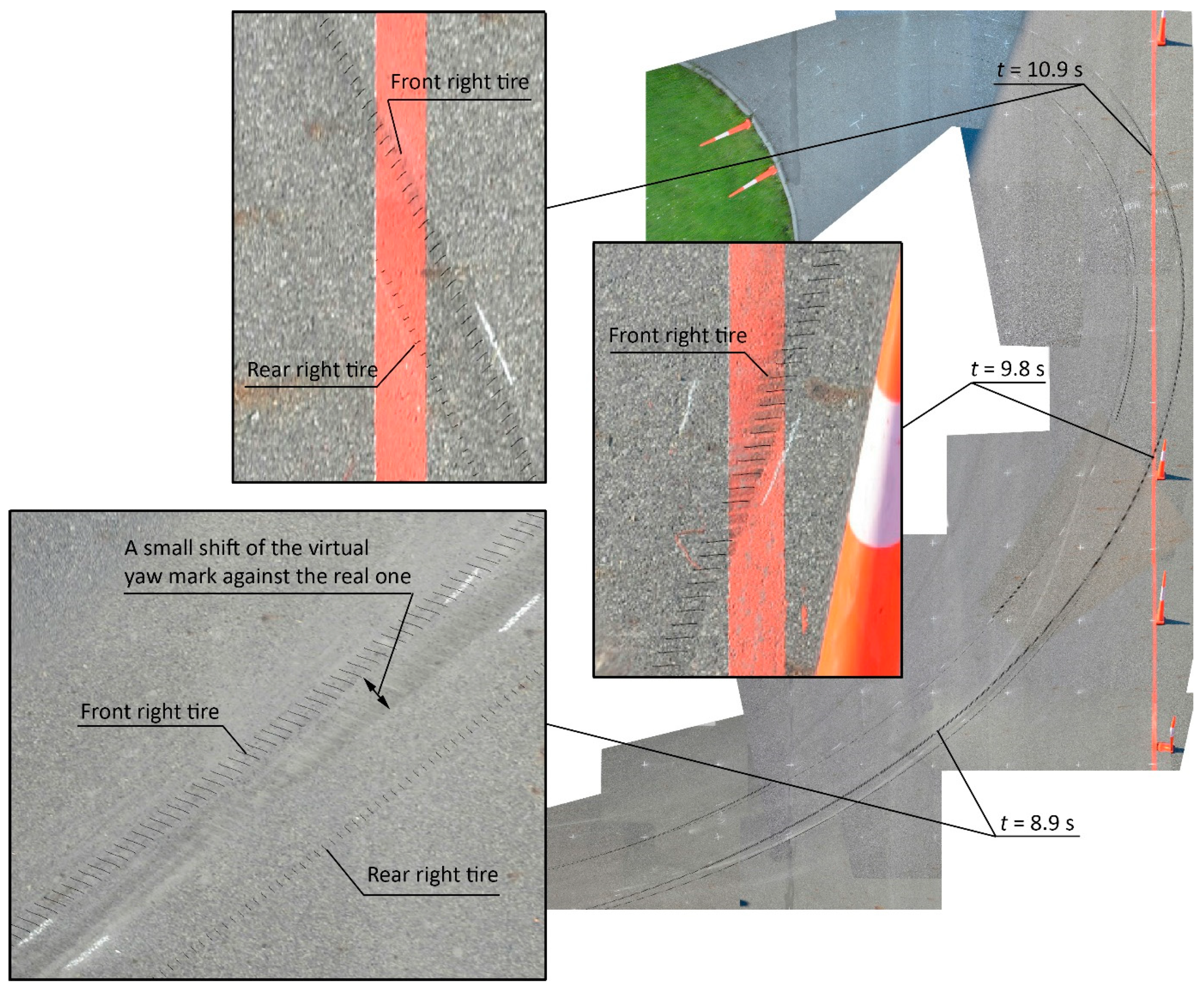
6.3. Stage 3. Verification of the Striation Creation Model

In Figure 11 the striated yaw marks generated in the simulation have been superimposed on the actual ones (note that on the orthophotomap you can also see irrelevant marks from earlier runs). There is a strong convergence in both the paths of the marks and the direction of the striations, as shown in the close-ups of the time points $t=$ 8.9 s, $t=$ 9.8 s and $t=$ 10.9 s. At $t=$ 8.9 s, the virtual mark of the front right wheel is slightly shifted to the right of the actual mark, but this is due to fact that the authors refrained from fine-tuning the simulation indefinitely.

6.4. Example

Figure 12 shows yaw marks generated in the simulation of a severe step steer in a left turn maneuver resulting in breaking the adhesion of the tires on the roadway and the vehicle yawing. Basically, this maneuver is similar to that of Section 6, but what is especially interesting here are typical yaw mark characteristics: variation of the width depending on the vehicle orientation with respect to the CG velocity direction, change of the striation angle with respect to the tangent to the yaw mark (straightening), interweaving and fading.

Remarks. The yaw mark creation model will still be valid on arbitrary 3D roads and typical road irregularities. Generally, bumps or potholes should result in gaps in the created yaw marks, but this problem has yet to be investigated.

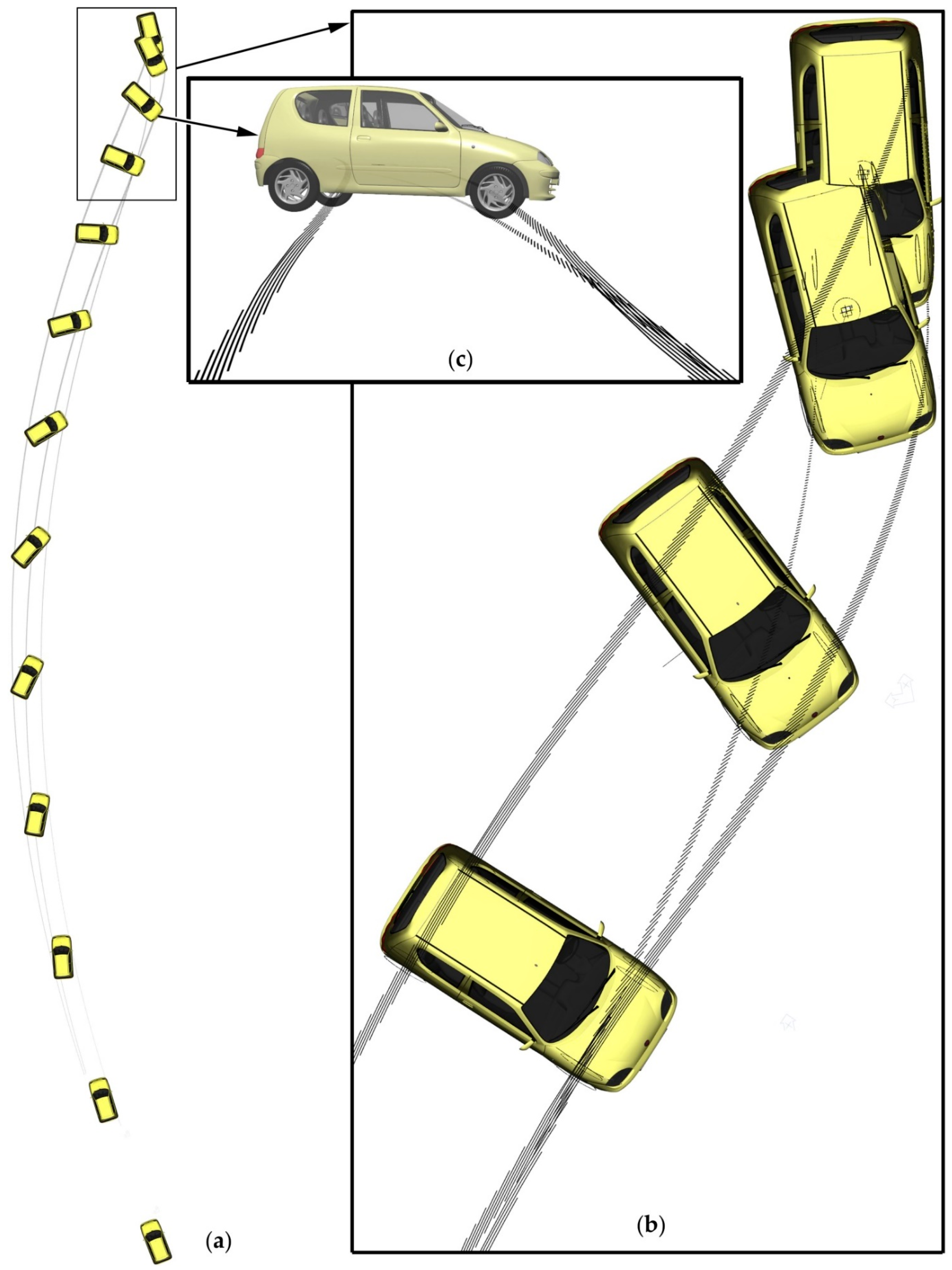
In case of uncommon suspension systems and/or different tire types, e.g., forklift trucks [25,26] or other uncommon vehicles [27], the response of the unsprung masses is not expected to affect the striated yaw mark creation model effectiveness as long as the vehicle is moving along a non-deformable surface and the road wavelength is not larger than the tire circumference.

7. Conclusions

• This work is, in some ways, a next step of the research of Beauchamp et al.—especially [13]. While they analyze striated yaw marks from the viewpoint of a reconstructionist who would like to know “what one can get from the marks uncovered at the accident scene” (deriving equations for calculation of longitudinal slip $s_x$ as a function of the striation marks angle $\theta$ and the slip angle $\alpha$), this work focuses on development of a model to create striated tire marks, which can be used in programs for simulation of vehicle accidents. While their formulas apply to planar mechanics and kinematics, this model takes into account the spatial vehicle multi-body dynamics and tire model, including the relative movement of the wheel, its position and orientation, tire deformation, suspension kinematics as well as forces and torques acting on the wheel. A mathematical model of striated tire yaw mark creation has been developed, intended for programs for the simulation of vehicle accidents. It implements the main features of the topology of such marks.
• The application of the model is twofold. The first one is the simulation of the formation of striated yaw marks. The second one is to facilitate the understanding of the mechanics of the formation of such marks and the inference of the braking or acceleration state of the wheels based on the topology of the striations.
• The mark creation model is universal, i.e., it applies to a tire moving along any trajectory with variable curvature, and it is subjected to any forces and torques calculated by solving a system of non-linear equations of vehicle dynamics.
• The striated yaw mark is created by the tread shoulder blocks forming the outer border of the contact patch, as this area is actually dominant.
• It is possible to define any, including non-uniform, pitch of the tread shoulder blocks.
• The striated yaw mark creation model can be applied in programs for the simulation of vehicle dynamics with any degree of simplification and any tire model. In this paper, it was validated using the author-developed program Model.exe, in which the vehicle is represented by a 36 degree of freedom multi-body system with the TMeasy tire model.

References

- Brach, R.M.; Brach, M. Vehicle Accident Analysis and Reconstruction Methods, 2nd ed.; SAE International: Pittsburgh, PA, USA, 2011; pp. 79–83. [Google Scholar]
- Sledge, N.H., Jr.; Marshek, K.M. Formulas for Estimating Vehicle Critical Speed from Yaw Marks—A review; SAE Technical Paper 971147; SAE International: Pittsburgh, PA, USA, 1997. [Google Scholar] [CrossRef]
- Cannon, J.W. A Study of Errors in Yaw-Based Speed Estimates Due to Effective Braking; SAE Technical Paper 2003-01-0888; SAE International: Pittsburgh, PA, USA, 2003. [Google Scholar] [CrossRef]
- Cliff, W.E.; Lawrence, J.M.; Heinrichs, B.E.; Fricker, T.R. Yaw Testing of an Instrumented Vehicle with and without Braking; SAE Technical Paper 2004-01-1187; SAE International: Pittsburgh, PA, USA, 2004. [Google Scholar] [CrossRef]
- Amirault, G.; MacInnis, S. Variability of Yaw Calculations from Field Testing; SAE Technical Paper 2009-01-0103; SAE International: Pittsburgh, PA, USA, 2009. [Google Scholar] [CrossRef]
- Lambourn, R.F. The calculation of motor car speeds from curved tyre marks. J. For. Sci. Soc. 1989, 29, 371–386. [Google Scholar] [CrossRef]
- Lambourn, R.F. Braking and Cornering Effects with and without Anti-Lock Brakes; SAE Technical Paper 940723; SAE International: Pittsburgh, PA, USA, 1994. [Google Scholar] [CrossRef]
- Lambourn, R.F.; Jennings, P.; Knight, I. Critical speed yaw mark calculations with and without electronic stability control. In Proceedings of the 1st joint ITAI–EVU Conference (18th EVU and 9th ITAI Conference), Hinckley, UK, 25–27 September 2009; ITAI–EVU: Hinkley, UK, 2009; pp. 209–235. [Google Scholar]
- Cash, S.; Crouch, M. Calculating vehicle speed from yaw mark analysis. In Proceedings of the 24th EVU Conference, Edinburgh, UK, 15–17 October 2015; EVU: Edinburgh, UK, 2015; pp. 185–206. [Google Scholar]
- Yamazaki, S.; Akasaka, T. Buckling behavior in contact area of radial tire structure and skid marks left by tires. JSAE Rev. 1998, 9, 51–55. [Google Scholar]
- Yamazaki, S. Friction coefficients of tires and skid marks left by tires. In Proceedings of the International Workshop on Traffic Accident Reconstruction, Tokyo, Japan, 12–13 November 1998; National Research Institute of Police Science: Chiba, Japan, 1998; pp. 41–51. [Google Scholar]
- Beauchamp, G.; Pentecost, D.; Koch, D.; Rose, N. The relationship between tire mark striations and tire forces. SAE Int. J. Trans. Saf. 2016, 4, 134–150. [Google Scholar] [CrossRef] [Green Version]
- Beauchamp, G.; Hessel, D.; Rose, N.A.; Fenton, S.J.; Voitel, T. Determining vehicle steering and braking from yaw mark striations. SAE Int. J. Passeng. Cars Mech. Syst. 2009, 2, 91–307. [Google Scholar] [CrossRef] [Green Version]
- Zębala, J.; Wach, W.; Ciępka, P.; Janczur, R. Determination of Critical Speed, Slip Angle and Longitudinal Wheel Slip Based on Yaw Marks Left by a Wheel with Zero Tire Pressure; SAE Technical Paper No. 2016-01-1480; SAE International: Pittsburgh, PA, USA, 2016. [Google Scholar] [CrossRef]
- Beauchamp, G.; Thornton, D.; Bortles, W.; Rose, N. Tire mark striations: Sensitivity and uncertainty analysis. SAE Int. J. Trans. Saf. 2016, 4, 121–127. [Google Scholar] [CrossRef]
- Guzek, M.; Lozia, Z. Computing methods in the analysis of road accident reconstruction. Arch. Comp. Meth. Eng. 2020. [Google Scholar] [CrossRef]
- Hirschberg, W.; Rill, G.; Weinfurter, H. Tire model TMeasy. Veh. Syst. Dyn. 2007, 45, 101–119. [Google Scholar] [CrossRef]
- Rill, G. Simulation von Kraftfahrzeugen; Vieweg & Sohn Verlag: Braunschweig/Wiesbaden, Germany, 1994. [Google Scholar]
- Pacejka, H.B. Tire and Vehicle Dynamics, 2nd ed.; SAE: Pittsburgh, PA, USA, 2006. [Google Scholar]
- Dugoff, H.; Fancher, P.S.; Segel, L. An Analysis of Tire Traction Properties and Their Influence on Vehicle Dynamic Performance; SAE Technical Paper No. 700377; SAE International: Pittsburgh, PA, USA, 1970. [Google Scholar] [CrossRef]
- Rill, G. Road Vehicle Dynamics: Fundamentals and Modeling; CRC Press: New York, NY, USA, 2012. [Google Scholar]
- Mitschke, M. Dynamik der Kraftfahrzeuge, Band A: Antrieb und Bremsung; Springer: Berlin/Heidelberg, Germany, 1995. [Google Scholar]
- Wach, W. Reconstruction of Vehicle Kinematics by Transformations of Raw Measurement Data. In Proceedings of the XI International Scientific and Technical Conference Automotive Safety, Častá, Slovakia, 18–20 April 2018. [Google Scholar] [CrossRef]
- Wach, W.; Struski, J. Rear wheels multi-link suspension synthesis with the application of a ‘Virtual Mechanism’. In SAE Special Publication SP-2019 Steering & Suspension Technology and Tire & Wheel Technology 2006; SAE Technical Paper No. 2006-01-1376; SAE International: Pittsburgh, PA, USA, 2006. [Google Scholar] [CrossRef]
- Martini, A.; Bonelli, G.P.; Rivola, A. Virtual testing of counterbalance forklift trucks: Implementation and experimental validation of a numerical multibody model. Machines 2020, 8, 26. [Google Scholar] [CrossRef]
- Rebelle, J.; Mistrot, P.; Poirot, R. Development and validation of a numerical model for predicting forklift truck tip-over. Veh. Syst. Dyn. 2009, 47, 771–804. [Google Scholar] [CrossRef]
- Odabaşı, V.; Maglio, S.; Martini, A.; Sorrentino, S. Static stress analysis of suspension systems for a solar-powered car. FME Trans. 2019, 47, 70–75. [Google Scholar] [CrossRef] [Green Version]