Resilience Assessment in Distribution Grids: A Complete Simulation Model

Abstract

For several years, the increase of extreme meteorological events due to climate change, especially in unusual areas, has focused authorities and stakeholders attention on electric power systems’ resilience. In this context, the authors have developed a simulation model for managing the resilience of electricity distribution grids with respect to the main threats to which these infrastructures may be exposed (i.e., ice sleeves, heat waves, water bombs, floods, tree falls). The simulator identifies the more vulnerable network assets by means of probabilistic indexes, thus suggesting the best corrective actions to be implemented for resilience improvement. The fulfillment of grid constraints, i.e., loading limits for branches and voltage limits for buses, under actual operating conditions, is taken into account. Load scenarios extracted from available measurements are evaluated by means of load flow analyses in order to choose, among the best solutions identified, those compatible with the constraints. The proposed tool can assist Distribution System Operators (DSOs) in drawing up the Action Plan to improve, on one hand, the resilience of the network and, on the other hand, to remove any possible limitation for the adoption of the best solutions to ensure maximum operational continuity during extreme weather events.

1. Introduction

PDNs are the part of the electric power system in charge of supplying final users, therefore being one of the main providers of goods and services to citizens. Moreover, the role of PDNs is expected to grow further in a smart city context. At the same time, the effect of electricity interruptions in PDNs has a huge impact on society, both in terms of quality of life and an economic point of view. For this reason, national governments classify PDNs as a critical infrastructure [1] and pay very much attention to their performance, both in normal operation and under extreme weather conditions. PDN performance under normal operation is evaluated by introducing well established reliability indexes [2], such as system average interruption duration index (SAIDI), system average interruption frequency index (SAIFI), loss-of-load expectation (LOLE), and electrical energy not supplied (EENS). However, the above reported reliability indices may not be satisfactory if the performance evaluation of PDNs must be made under extreme weather conditions, i.e., if PDN resilience has to be assessed.

In literature, a certain number of metrics have been proposed to assess critical infrastructure resilience, following either a qualitative approach or a quantitative one: the interested reader may refer to [3]. Regarding electrical power systems, quantitative metrics (both deterministic and probabilistic metrics) are more suitable and have been proposed. In some cases, reliability indices have been used to assess resilience, such as the availability in [4], which is specifically focused on PDNs, or LOLE and EENS in [5], which considers HV transmission systems. Complex network metrics have been proposed in [6] and applied to the Korean power grid. Also, [7] quantifies resilience of PDNs using complex network metrics, but at the same time proposes a decision-making resiliency quantification tool and thus obtains combined indices based on network percolation theory and complex network analysis. A time-dependent resilience metric is presented in [8] for urban infrastructure systems, which has been used by [9] for the probabilistic assessment of PDN resilience, taking into account different weather scenarios by means of Monte Carlo simulations. Reference [10] introduces the concept of spatial dependence within infrastructure systems, pointing out the interaction between PDN and the biophysical environment. For instance, vegetation plays an important role in PDNs resilience, and the proximity to high priority emergency assets increases resilience of the involved portions of PDN. A very useful review on existing studies related to PDN resilience assessment and improvement is provided in [11], which also proposes an optimal distributed generation islanding strategy considering PDN reconfiguration, in order to improve resilience after multiple faults.

Despite the continuously increasing interest, a framework with simple metrics allowing practical applications in order to evaluate PDN resilience and improve supply performance is, at present, still lacking. Moreover, most of the resilience metrics practically used by DSOs are established by government agencies or utilities, such as the ones involved in critical infrastructure resilience in the United States and in the European Community [12,13,14,15,16] and, more specifically, in electric power system resilience [16]. In Italy, ARERA (acronym, in Italian, of Regulatory Authority for Energy, Networks and Environment) [17] provided some guidelines [18] to DSOs for assessing PDN resilience in case of extreme natural events, such as heavy snowfalls, heat waves, floods and windstorms. Moreover, based on the obtained results, DSOs are in charge of developing plans aimed at improving network resilience against extreme natural events, in order to reduce the global impact of electric service failures during these threats. The approach in [18] is probabilistic, based on the calculation of failure probability of MV power lines and the related damage, measured as the number of LV customers disconnected in a given RT assigned to the MV line for each specific threat. A more detailed description of the ARERA approach is given in [19,20,21,22,23] for different extreme natural events, as well as the methodologies developed by DSOs for assessing RTs of each asset of the MV distribution network involved.

The approach in [18] is static: only the MV distribution network topology has to be represented and the network resilience only depends on the number of disconnected LV customers rather than the actual electrical parameters of the grid. For this reason, network constraints are not taken into account, so that the occurrence of overloads during degraded service conditions is not checked, and the possible occurrence of cascading failures is not investigated. This paper presents a simulation model able to assess PDN resilience under the action of extreme weather events, such as flooding, ice sleeves, heat waves and tree fall, on all assets of the PDN. Starting from the static resilience index introduced in [18], resilience is calculated by considering load profiles over time and checking the possible violations of network constraints, i.e., branch ampacities and bus voltage violations, by means of power flow calculations performed for the entire PDN. Three additional indexes are also proposed. The simulation model is applied to the existing PDN in Terni, a city in the center of Italy, owned by A.S.M. Terni S.p.A. and operated by TDE.

The main contribution of the paper is to provide a tool through which a DSO may assess in a practical way the resilience of its PDN and easily identify the remedial actions required to increase grid resilience against specific threats. On one hand, different to many approaches proposed by academia, which are mostly theoretical and/or difficult to implement by utilities in a real setting [4,24], the tool allows evaluation of PDN resilience by using information and data usually available to a DSO. On the other hand, oversimplifications usually associated with resilience metrics established by national authorities or agencies are avoided.

This paper is structured as follows. Section 2 discusses the resilience index and the additional proposed indices, as well as the calculation of RTs for each considered threat; the methodology for resilience evaluation when load profiles and violation of network constraints are taken into account is also addressed. Section 3 shows and discusses the results obtained by the proposed model when applied to the existing PDN in Terni; the main differences in case load profiles and network constraints that are not taken into account are also highlighted. Lastly, conclusions are presented in Section 4.

2. The Simulation Model

This section describes the complete simulation model proposed by the authors to assess the resilience of MV PDNs. The network is modelled as a graph composed by buses and branches, representing all possible assets in a PDN. Buses are busbars of the PSs connecting the MV PDN to the HV system; MV busbars of SSs supplying LV users; MV busbars of privately owned secondary substations supplying MV users; MV busbars of sectionalizing substations; and stiff connections of MV overhead lines. Branches are MV feeder stretches connecting two MV buses; HV/MV transformers installed at PSs; MV/MV transformers connecting grid portions at different voltage levels (if any); switches; and busbar couplers.

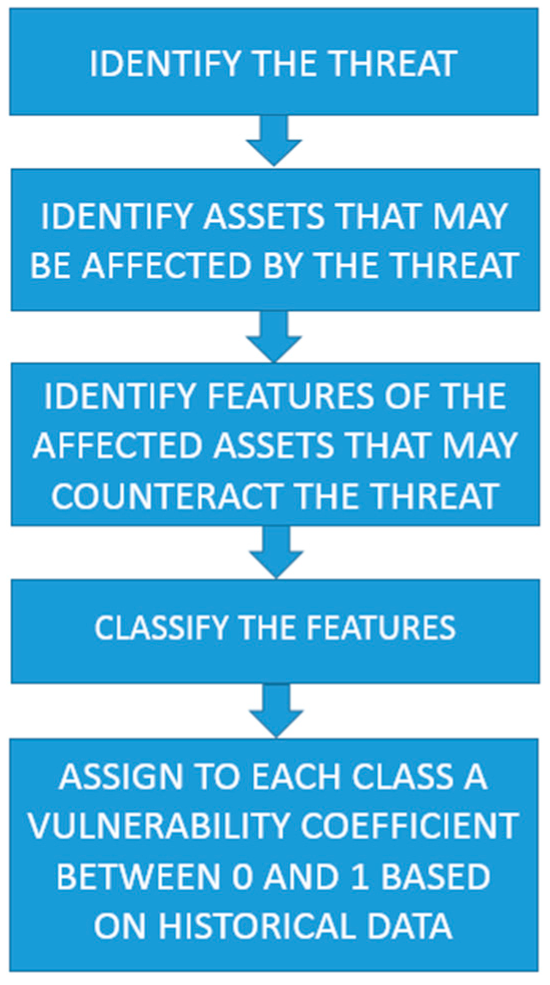
2.1. Risk and Resilience Indexes

In [18], the Italian Authority ARERA provides a methodology to perform the resilience analysis of a PDN. The approach is based on the RT, defined as the average time span between two consecutive events due to the same threat, and on the magnitude of damage caused by the event, defined as the NUD from the PDN due to the event occurrence. A RT value is assigned to each network asset; the inverse of RT is the probability that the asset is disconnected due to the occurrence of the threat. The risk index I_risk is thus defined as the product between the probability of asset disconnection and NUD, whereas the resilience index I_resilience is defined as the inverse of I_risk. The evaluation of RT for each asset depends on the specific threat considered and will be addressed in Section 2.3 in the case of ice sleeves, heat waves, flooding and tree fall. In case of flooding and heat wave threats, moreover, the RTs also depend on vulnerability coefficients, which are determined empirically by operational experience, as explained in Section 2.3. Figure 1 reports a flow chart summarizing the general methodology used in this paper to evaluate vulnerability coefficients.

Since the disconnection of one asset may be caused by the disconnection of another asset (for instance, a SS may be disconnected due to a fault on an MV feeder stretch), the concept of RT_eq is introduced. RT_eq is calculated as the minimum RT amongst the RTs of all assets that cause the disconnection due to the threat occurrence. RT_eq is thus used to evaluate both I_risk and I_resilience by the following expressions:

I_risk = RT_eq⁻¹·NUD,

(1)

I_resilience = I_risk⁻¹ = RT_eq·NUD⁻¹.

(2)

2.2. Additional Indexes

In addition to indexes defined in [18], the authors proposed in previous works [20,21,22,23] three additional indexes able to evaluate the global performance of a PDN in terms of resilience: the network global resilience index (I_NGR), the network reconfiguration index (I_NR) and the users vulnerability index (I_UV).

I_NGR is calculated as

$${\mathrm{I}}_{\mathrm{NGR}}=\frac{\left[{\displaystyle {\sum }_{\mathrm{i}}\left(1-\frac{1}{\mathrm{R}{\mathrm{T}}_{\mathrm{eq},\mathrm{i}}}\right)}\cdot {\mathrm{NCU}}_{\mathrm{i}}\right]}{\mathrm{NTU}},$$

(3)

where NCU_i is the number of users connected at bus i and NTU is the number of total users supplied by the PDN; the summation is extended to all buses of the grid. I_NGR depends on the specific threat considered, since in Equation (3) RT_eq,i of bus i is involved, and its value may vary in the range 0–1: 0, this means that all users are disconnected to the grid due to the threat; 1 means that no user is disconnected.

I_NR is calculated as

$${\mathrm{I}}_{\mathrm{NR}}=\frac{{\displaystyle {\sum }_{\mathrm{i}}\mathrm{k}\cdot {\mathrm{NCU}}_{\mathrm{i}}}}{\mathrm{NTU}},$$

(4)

where k is a numerical coefficient equal to 1 if it is possible to reconfigure the network in order to supply bus i, 0 otherwise; the summation is extended to all buses of the grid. Also, this index may vary in the range 0–1, and I_NR = 1 means that there is always at least one network reconfiguration able to supply all network buses.

Lastly, I_UV is calculated as

$${\mathrm{I}}_{\mathrm{UV}}=\frac{{\displaystyle {\sum }_{\mathrm{j}}{\mathrm{NUD}}_{\mathrm{j}}}}{\mathrm{NTU}},$$

(5)

where NUD_j is the number of users disconnected due to the disconnection of branch j, and the summation is extended to all network branches. In this case, the greater the I_UV, the larger the user vulnerability, i.e., the lower the network performance against the considered threat; moreover, note that I_UV may be greater than 1.

The proposed additional indexes are useful:

• to evaluate the performances of a PDN under different threats;
• to compare performances of different PDNs;
• to identify the most suitable remedial actions in order to improve the network resilience.

2.3. RT Assessment

The evaluation of RT for each network asset and, consequently, of RT_eq for each bus of the grid, is dependent upon the specific threat considered. In this subsection we present the RT evaluation performed for four different threats, namely ice sleeve formation, heat waves, flooding and tree fall.

2.3.1. Ice Sleeve Formation

In case of ice sleeve threat, the PDN assets involved are MV overhead lines; moreover, the availability of PSs and possible interconnections with other MV networks must also be taken into account.

As regards MV overhead lines, RT is calculated according to European [25] and Italian [26] standards. References [25,26] establish sizing criteria for electrical overhead lines with nude conductors to ensure a standard 50 year RT, considering the overall mechanical stress due to ice load and wind by means of the Gumbel statistical distribution [27]. Prescriptions in [25,26] are applicable to newly built MV and HV overhead lines, but at the same time allow assessment of RT values of already existing overhead lines based on mechanical features and geographical areas of installation. Moreover, for a more accurate RT estimation, updated meteorological datasets at a municipal level may be used to revise, over time, information about new recorded yearly ice load values. The assumption made for this methodology is that climatic parameters such as temperature and wind speed are uniform all over the PDN.

With respect to HV busbars of PSs, the RT value assessment should be made by the TSO and provided to the DSO, since such datum depends on the HV system resilience. In case of lack of data provided by the TSO, the DSO may only perform a rough estimate based on operational experience. The subject is the same in case RT values of existing interconnections with MV networks operated by other DSOs have to be calculated.

2.3.2. Heat Waves

In case of heat wave threat, it is assumed that only SSs may be affected. RT values to assign to each SS depends on two quantities: the return time of heat wave threat itself, and the fault probability of the SS in case the heat wave occurs, henceforth called heat wave vulnerability.

A heat wave is defined as a period of consecutive days with temperatures excessively higher than usual. The TX3X quantity is considered, following the work reported in [28]. This may be done by available measurements of ambient temperatures: in case of TDE’s PDN, official temperature data released by the observatory “Federico Cesi”, located in Terni, have been used. It is assumed that a 34 °C TX3X is a severe condition for the heat transfer inside the SS, thus yielding an RT of about 17.7 years for the city of Terni following the approach in [28].

Regarding SS heat vulnerability, an empirical approach based on DSO’s experience and know-how is followed. A heat wave vulnerability coefficient K_V,HW, varying in the range between 0 and 1, is assigned to each SS. K_V,HW is calculated as the product between a fragility coefficient due to the SS typology, K_F,SS, and a fragility value, K_F,MVP, due to the typology of the MVP installed in the substation. By multiplying the inverse of K_V,HW and the RT value of the heat wave event, RT values of SSs are obtained.

Seven different substation typologies are identified, namely:

• tower Substation—Type 1;
• undergrounded Substation—Type 2;
• pole Mounted Distribution Transformer—Type 3;
• prefabricated Substation—Type 4;
• building Undergrounded Substation—Type 5;
• box Substation—Type 6;
• raised Prefabricated Substation—Type 7.

For each substation type, a specific K_F,SS value is established, reflecting the fact that different heat transfers occur (for instance, a pole mounted distribution transformer is expected to have a more efficient heat transfer than an underground substation). K_F,SS values assigned to each SS type are reported in

Table 1. K_F,SS values for SS typology.

Substation Typology	Fragility
Type 1	0.25
Type 2	0.75
Type 3	0.25
Type 4	0.5
Type 5	0.25
Type 6	0.5
Type 7	0.25

.

Since the behavior of an SS when a heat wave occurs depends also on the MVP installed, three different types of MVPs have been identified, namely:

• SF₆ insulated MVP—Type 1;
• protected MVP—Type 2 (modular blocks designed for protecting lines and transformers, widely installed in distribution networks);
• air insulated MVP—Type 3.

Regarding K_F,MVP coefficients, it is assumed that air insulated MVPs are less efficient and more vulnerable to severe thermal transients, whereas SF₆ insulated MVP are the less vulnerable; an intermediate behavior is assumed for protected MVP. The K_F,MVP values assigned to each MVP type are reported in

Table 2. K_F,MVP values for MVP typology.

MVP Typology	Fragility
Type 1	0.4
Type 2	0.7
Type 3	0.9

. Assuming 17.7 years RT for heat waves,

Table 3. RT values (years) of SS outage in case of heat waves.

Substation Typology	MVP Typology
	Type 1	Type 2	Type 3
Type 1	177.99	101.71	79.11
Type 2	59.33	33.91	26.36
Type 3	177.99	101.71	79.11
Type 4	88.99	50.85	39.55
Type 5	177.99	101.71	79.11
Type 6	88.99	50.85	39.55
Type 7	177.99	101.71	79.11

reports RT values to assign to each SS in TDE’s PDN, taking into account both SS and MVP typology.

2.3.3. Flooding

In case of flooding threat, the assumption that only SSs are affected is made. As for heat wave threat, RT values to assign to each SS depends on two quantities: the return time of flooding threat itself, and the fault probability of the SS in case a flooding occurs, henceforth called flooding vulnerability.

The probability of the flooding event may be easily assessed by using data provided by authorities supervising hydrogeological basins, which moreover directly evaluate RTs of floods in the respective basin. In the case of TDE’s PDN, the hydrogeological risk plan drawn up by the Province of Terni and Tiber River Basin Authority [29,30] have been used. The authority identifies four different zones, each characterized by a specific hydrogeological risk with an associated RT:

• Zone A: high hydrogeological risk, 50 years RT;
• Zone B: medium hydrogeological risk, 200 years RT;
• Zone C: low hydrogeological risk, 500 years RT;
• Zone D: no hydrogeological risk, RT = ∞.

Such zones, as well as the location of SSs in the TDE’s PDN, are evidenced in Figure 2.

In cases where an acceptable number of historical data correlating floods and SS faults is available, fragility curves could be obtained following the approach in [31]. Otherwise, an empirical approach may be adopted, assigning a flood vulnerability coefficient K_V,F to each SS of the network in order to estimate the probability that a flooding may cause the SS outage. K_V,F can vary between 0 and 1 and depends on SS typology; values proposed in this paper are:

• K_V,F = 1 for underground substations, i.e., a flooding always cause the SS disconnection;
• K_V,F = 0.75 for substations installed inside buildings, boxes, and prefabricated systems, i.e., a flooding may partially affect the SS;
• K_V,F = 0 for the SSs raised off the ground, as in the case of pole mounted distribution transformers, i.e., the probability that a flooding causes the disconnection is null.

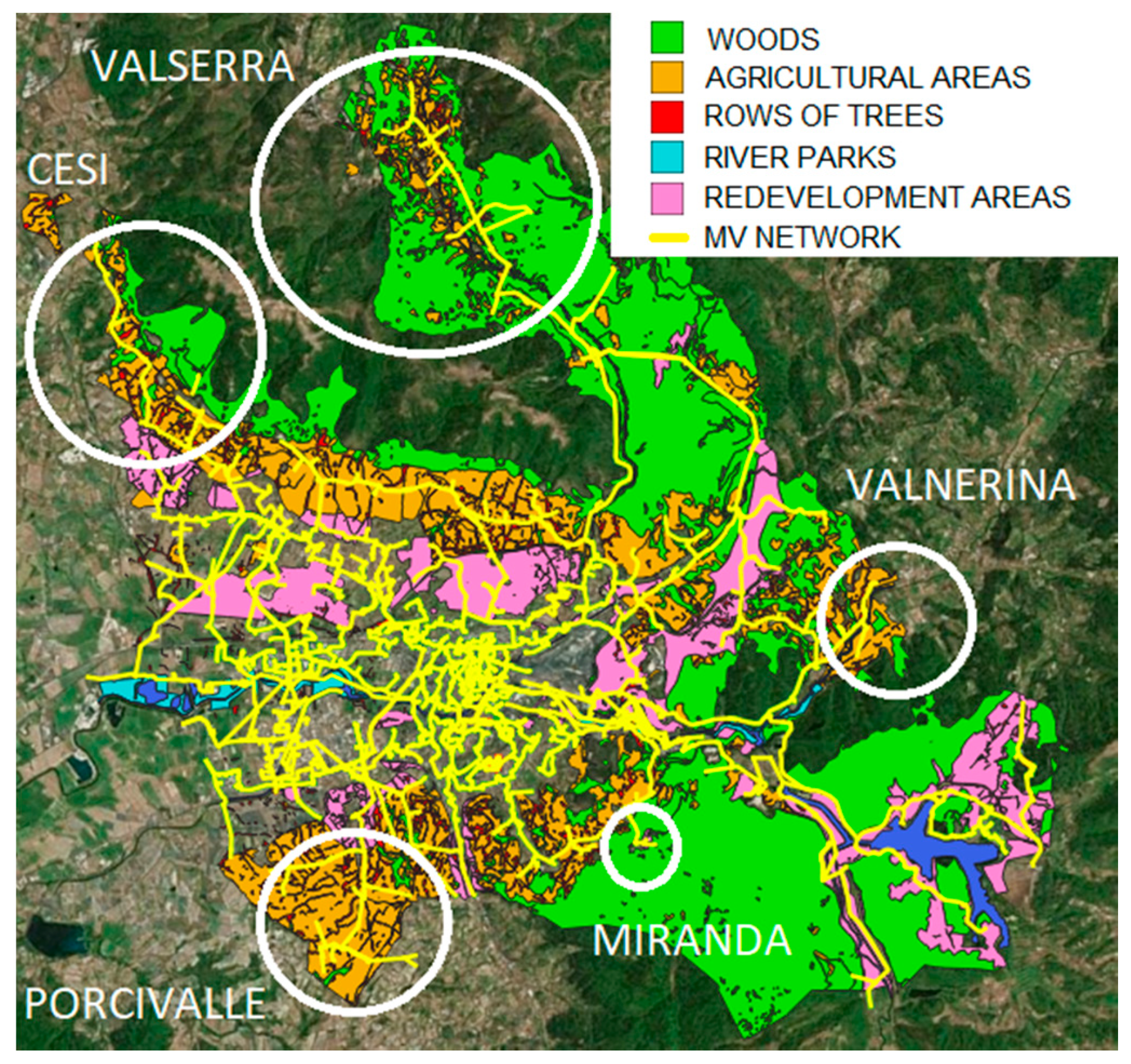
By dividing the flooding RT over K_V,F for each SS, RT of SSs in case of flooding threat is obtained. In case RT = ∞, an arbitrarily large enough RT value could be selected.

2.3.4. Tree Fall

It is assumed that only overhead lines may be affected by tree falls. In order to assess RT due to tree fall, a detailed characterization of the territory where overhead lines are located, as well as recordings concerning tree fall events able to cause the interruption of the electricity supply, are needed.

The territory covered by a PDN may be subdivided with respect to tree fall threat in different subareas: such characterization may be obtained, for instance, from the city’s land-use plan. In order to explain better the proposed methodology, the city of Terni is taken as an example. In the area covered by the TDE’s PDN, five different subareas may be identified:

• woods;
• agricultural areas;
• rows of trees;
• river parks;
• redevelopment areas.

By using the Geographical Information System (GIS) environment, a map is obtained and the PDN is overlapped on the map in order to obtain the incidence of each subarea (in terms of length) on lines of the PDN. The concept of TCL of each overhead line is introduced, considering different weight factors for the previously defined subareas:

• TCL for an overhead line in woods is equal to the real line length;
• TCL for an overhead line in agricultural areas is obtained by multiplying the line length by 0.3;
• TCL for an overhead line crossed by rows of trees is obtained by assigning to each tree crossing an equivalent length equal to 50 m;
• TCL for an overhead line in river parks is obtained by multiplying the length by 2;
• TCL for an overhead line in redevelopment areas is obtained by multiplying the length by 0.7;
• TCL for an overhead line outside the five areas is zero (i.e., urban areas).

By summing up all of the calculated TCLs, the ATCL of the PDN is obtained.

In order to obtain TR values for tree fall threat, recordings of tree fall events able to cause supply interruptions (which are available amongst the recordings of the Perturbed Condition Periods) are used. If N_faults is the number of such events recorded in a N_years time period, quantity δ is at first calculated:

$$\mathsf{\delta }=\frac{{\mathrm{N}}_{\mathrm{faults}}}{{\mathrm{N}}_{\mathrm{years}}}.$$

(6)

Using the ATCL (km), the PDN fault rate per kilometer τ_f,km (faults·years⁻¹·km⁻¹) is evaluated:

$${\mathsf{\tau }}_{\mathrm{f},\mathrm{k}\mathrm{m}}=\frac{\mathsf{\delta }}{\mathrm{ATCL}}.$$

(7)

Defining the return time per kilometer (RT_km) as the inverse of τ_f,km, RT of each overhead line (years·faults⁻¹) may be finally obtained:

$$\mathrm{RT}=\frac{{\mathrm{RT}}_{\mathrm{km}}}{\mathrm{TCL}}.$$

(8)

Figure 3 shows the map of the subareas defined for the municipality of Terni, as well as the overlapped MV PDN; the most critical PDN sections with respect to tree fall (i.e., low RT values) are also highlighted.

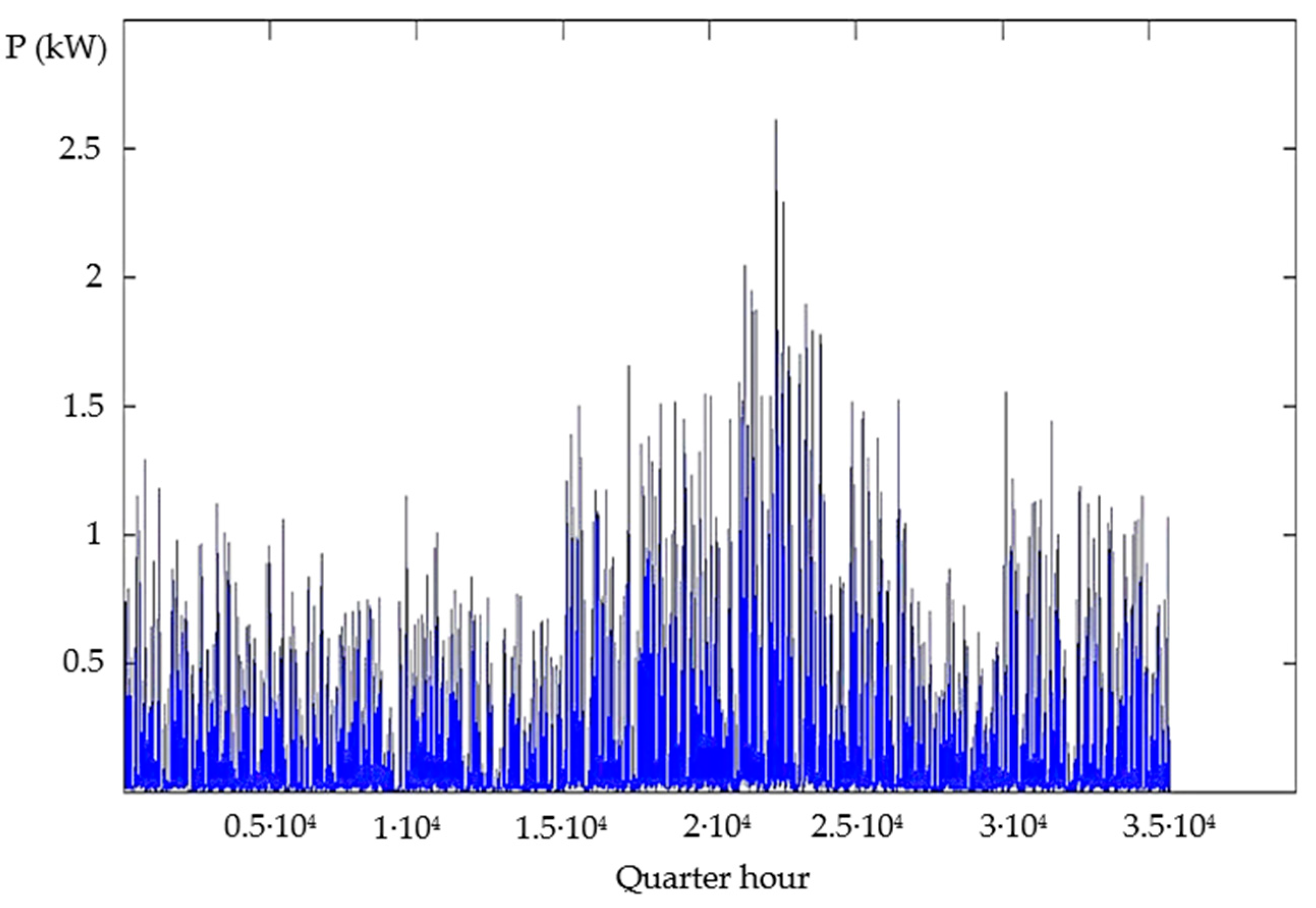
2.4. Creation of Network Load Scenario

Both LV and MV loads connected to the distribution networks are simulated as balanced loads. For each user connected at MV level and for a part of users connected at LV level, TDE has made available the consumed/produced electrical energy, measured by smart meters each quarter hour at the point of delivery. In this case, the load profile is obtained simply by calculating the equivalent constant power load for each quarter hour and saving this in a database.

If energy measurements every 15 min are lacking, which is the case for most LV users connected to TDE’s distribution grid, the monthly aggregated energy measurements available for each LV user are used to estimate load profiles. LV users are subdivided in different classes based on the contractual power. For each class two reference, daily load profiles, referred to by the days of maximum and minimum load conditions with a 15 min resolution, are available. Daily load profiles are created for each user by generating randomly a quarter hour power value between the corresponding values of the minimum and maximum load profiles. Power values are then weighted in order to match the monthly aggregated energy consumption and, lastly, profiles are smoothed by means of the moving average technique. Applying the procedure to each month of the year, a yearly load profile with a quarter hour resolution is generated for each LV user and saved in a database. Figure 4 plots a yearly load profiles generated for an LV user with a 3 kW contractual power.

Both generated and measured load profiles are then read from the database and aggregated in the respective buses of the PDN which users are connected to. In such a way, the complete yearly load scenario of the PDN with a quarter hour resolution is obtained.

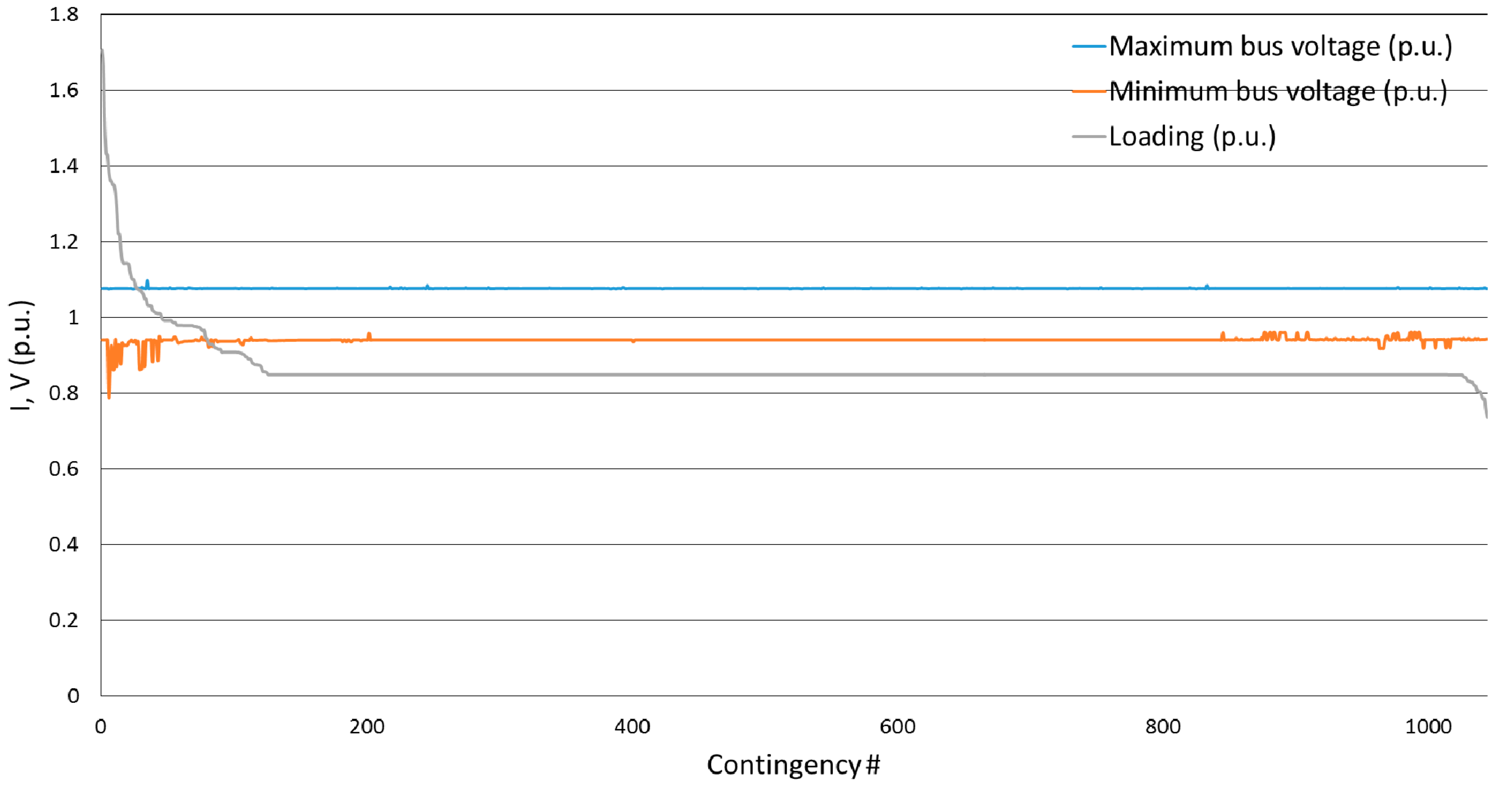
2.5. Selection of Reference Critical Scenarios

A typical radial layout of the PDN is selected for the entire yearly load scenario. Further, 35040 load flow simulations (one for each quarter hour of the year) are performed checking that network constraints (branch loadings and bus voltages) are never violated, thus validating the correctness of the created network load scenario.

In order to take into account different load conditions in PDN resilience assessment, N_RCS = 9 reference critical load scenarios are selected amongst the 35040 quarter hour load profiles:

• three scenarios corresponding to the maximum loading of three different branches;
• one scenario corresponding to the maximum average loading of all the branches;
• one scenario corresponding to the minimum average loading of all the branches;
• one scenario corresponding to the maximum bus voltage;
• one scenario corresponding to the minimum bus voltage;
• one scenario corresponding to the maximum voltage variance of all buses;
• one scenario randomly selected amongst the remaining quarter hour scenarios.

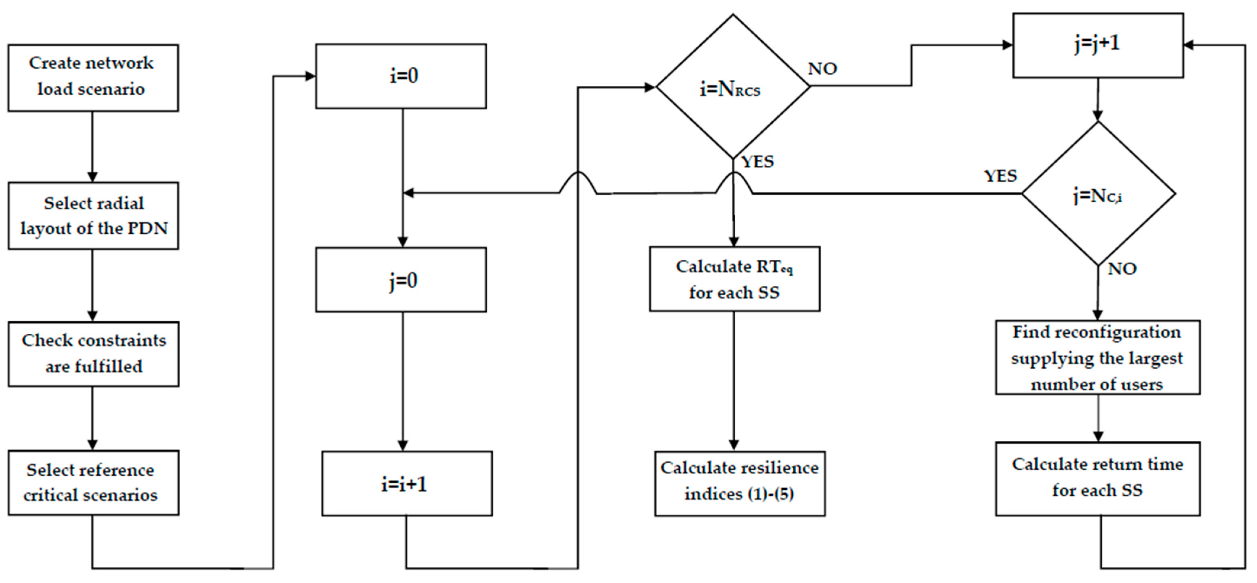
2.6. Resilience Assessment Procedure

Reference critical scenarios are inputs of the complete simulation model. For each scenario i, a set of contingencies N_C,i is sequentially analyzed. Each contingency is represented by the disconnection of one network asset, i.e., a node or a branch of the PDN; different possible contingencies are associated to each threat, as listed below:

• Ice sleeves: branches representing MV overhead lines; nodes representing interconnections with HV network; nodes representing interconnections with other MV networks.
• Heat waves: nodes representing the MV busbars of the SSs.
• Floodings: nodes representing the MV busbars of the SSs.
• Tree fall: branches representing MV overhead lines.

For each contingency, a rerouting algorithm is applied in order to find the network configuration able to supply most users. The rerouting algorithm behaves similarly to an operator in the control room: only switches available in the portion of the PDN involved in the contingency may be switched on/off, as in real time operation. At this stage, although all network reconfigurations allow connecting all users to the PDN, network constraints are taken into account: overloaded branches and/or buses with voltage outside the voltage range between 90% and 110% of the rated voltage are disconnected. For each contingency, the RT value assigned to each SS is the lowest between RT values of the assets whose disconnection causes the SS disconnection. When all of the contingencies of all reference critical scenarios are simulated, RT_eq of each SS is simply the lowest RT. At this point, calculation of indexes (1) and (2) for each SS, as well as of indexes (3)–(5) for the entire PDN, is performed.

The proposed simulation model is outlined in the flow chart depicted in Figure 5.

The main advantage of the proposed procedure is that only data normally at disposal of a DSO are required, thus allowing the evaluation of indexes (1)–(5) in a viable way. However, some aspects related to resilience are not, or are only marginally, addressed by the procedure. Taking as a reference the four resilience functions proposed by [32], namely ‘resist’, ‘re-stabilize’, ‘rebuild’ and ‘reconfigure’, the procedure is mainly focused on the first two functions. The speed of load restoration to the pre-event level after the threat, represented by the function ‘rebuild’, is not covered by indexes (1)–(5). As regards the ‘reconfigure’ function, which represents the actions that have to be taken in order to improve resilience, RT_eq values yielded by the procedure give the DSO a clear view of weakest assets of the network, but the optimal investment plan is not provided. Such aspects will be the object of further studies aimed at realizing a comprehensive tool with respect to power distribution network resilience.

3. Results

In this section, a case study regarding the resilience assessment against tree fall in the existing PDN in Terni, owned by ASM and operated by TDE, is described. Main results are reported and differences obtained when considering load profiles and network constraints, with respect to the pure topological approach coded by ARERA in [18], are highlighted.

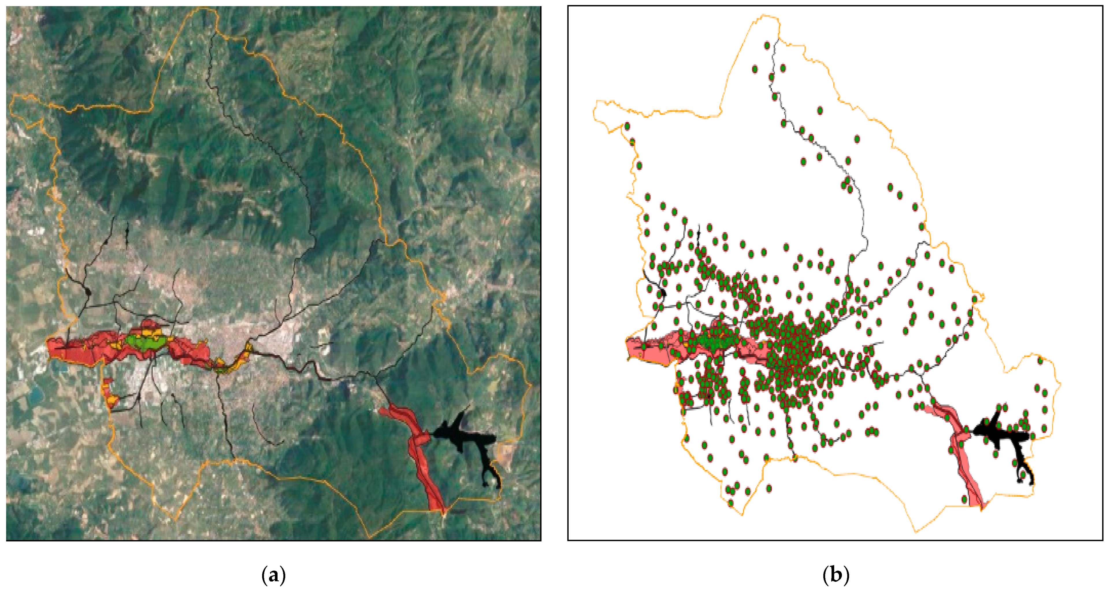
3.1. PDN under Study

The PDN is connected to the Italian HV network by three primary substations, each one with two HV/MV transformers installed; a seventh HV/MV transformer is installed as a spare transformer. There are also eight interconnections with other PDNs owned by other DSOs. The network is operated at two voltage levels, namely 10 kV and 20 kV: the portions at different voltage levels are interconnected by means of six MV/MV substations. Also, 588 SSs are installed for an aggregate 127 MVA installed power, supplying about 65,000 LV customers (for an aggregate 250 MW contractual power); the average daily consumption is about 890 MWh. A SCADA system is installed, connected to and remotely controlling 96 SSs. The MV distribution network is about 640 km long, composed by overhead lines (about 62.2%) and underground cables (about 37.8%), and covers an area of about 212.5 km² of the Terni territory. Lastly, a considerable amount of distributed generation is installed in the PDN (this is also the reason why the reference critical scenario concerning maximum bus voltage is evaluated):

• thirty-one MWp photovoltaic plants, producing about 36 GWh yearly;
• seven Hydro plants for an aggregate 10 MW power, producing about 68 GWh yearly;
• four biomass/waste to energy plants for an aggregate 20 MW power, producing about 78 GWh yearly.

Previously reported Figure 2 and Figure 3 show the PDN topology and its displacement in the Terni territory.

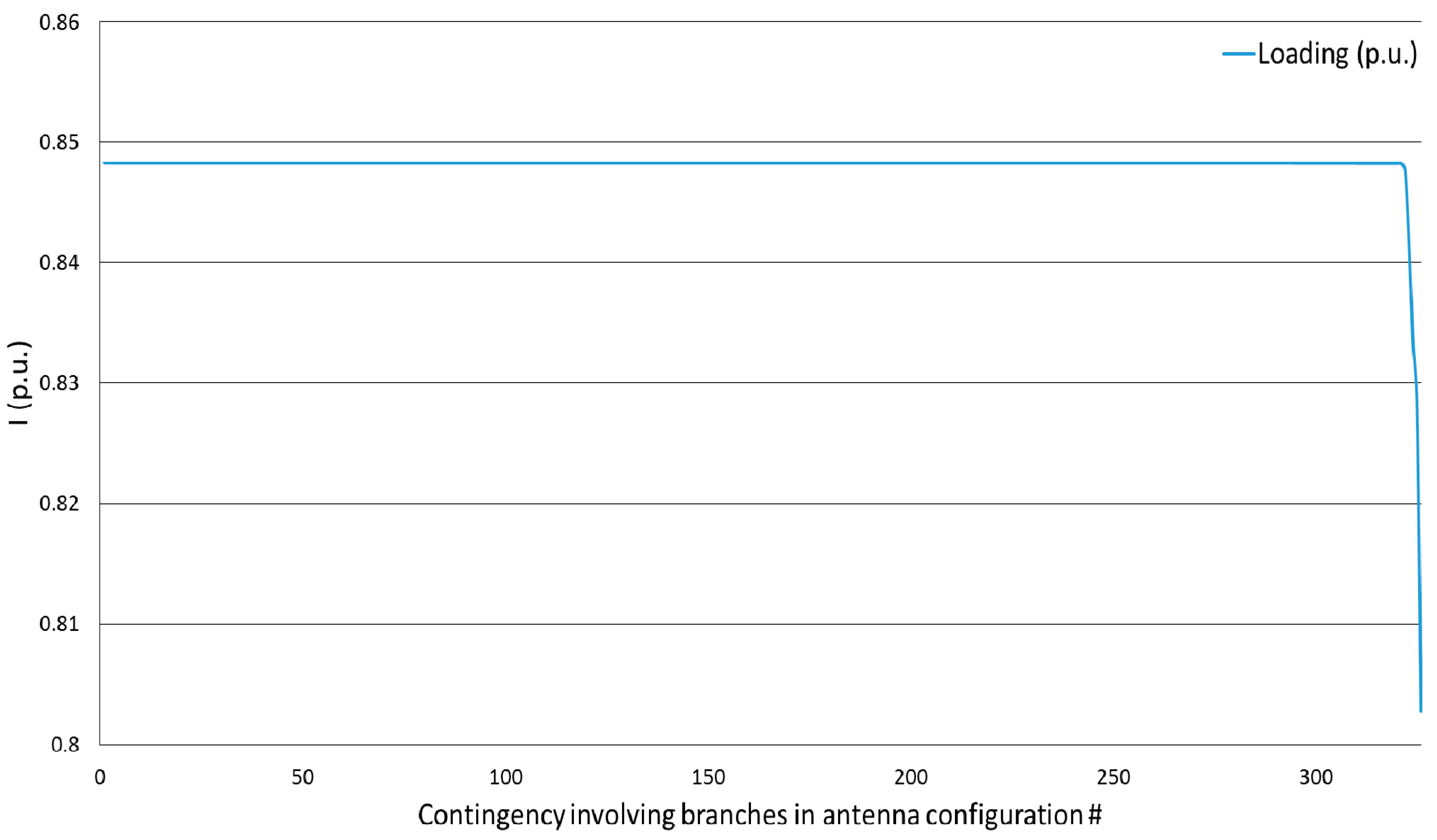
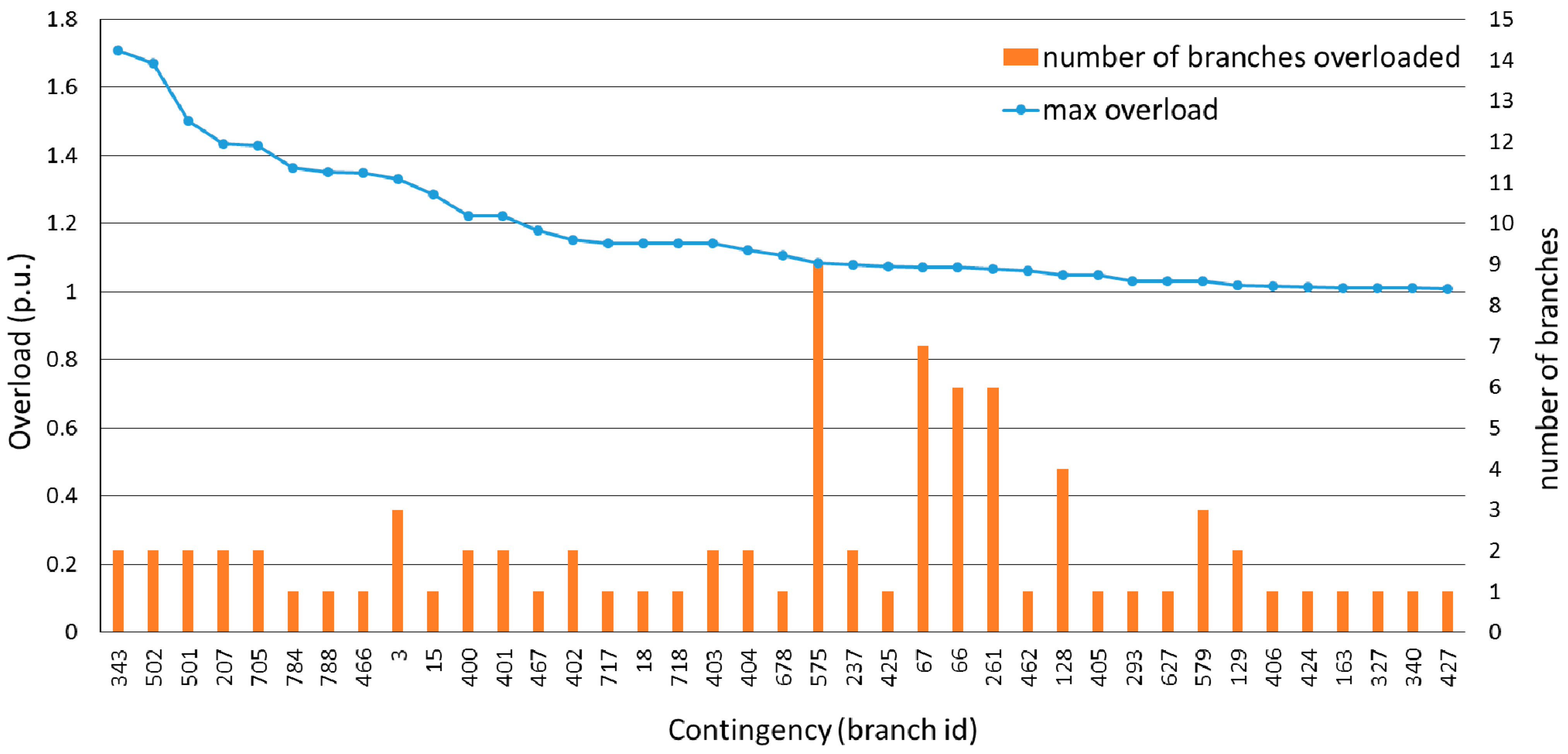
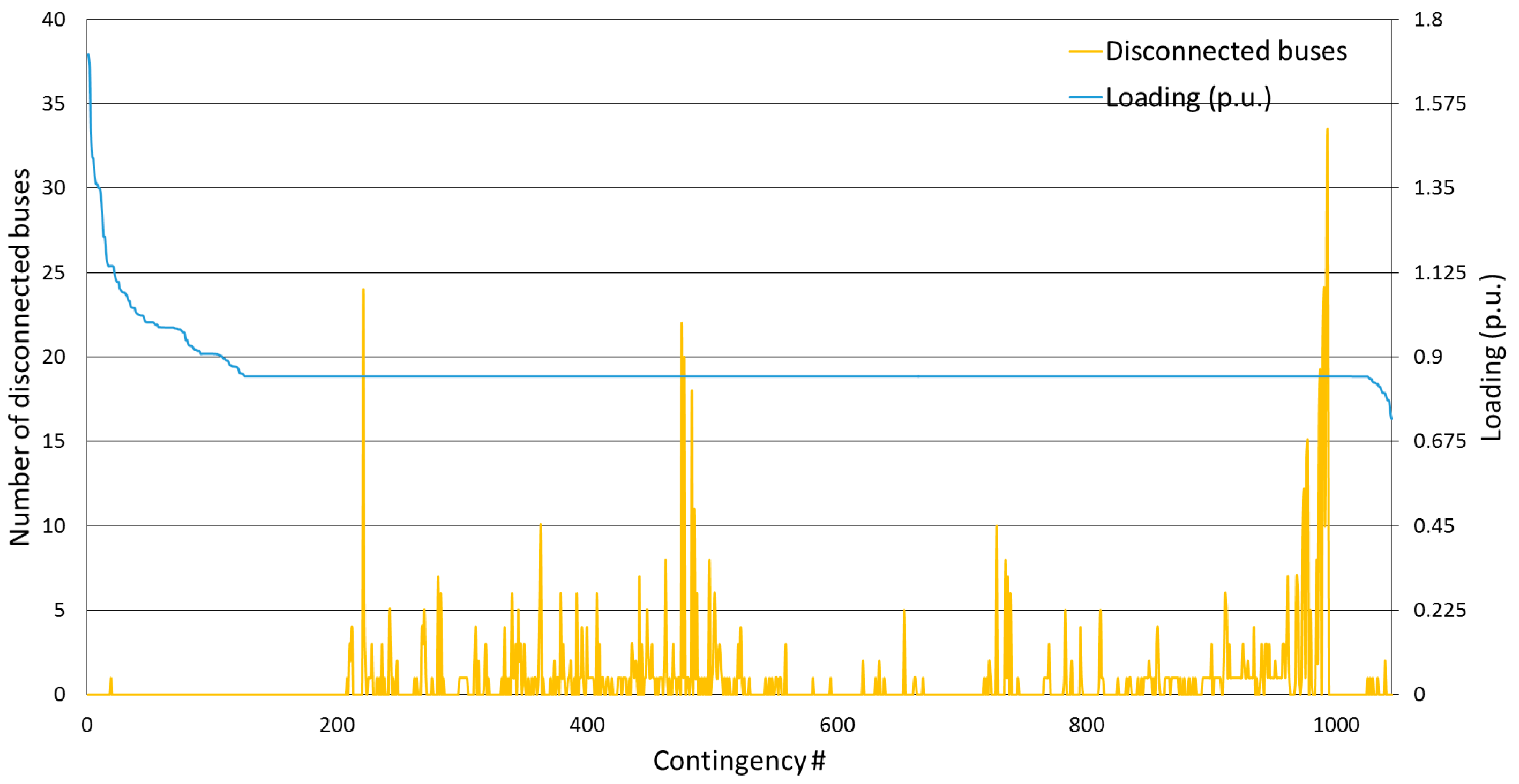
3.2. Numerical Application: PDN Resilience against Tree Fall

The procedure is applied to assess the PDN resilience in case of tree fall threat. TCL of each branch is at first calculated, and then TCLs of all branches are totaled, obtaining ATCL = 101.5 km (which is about 15.86% of the aggregate 640 km PDN length). From recordings available in the Perturbed Condition Periods, N_faults = 20 and N_years = 12, thus obtaining δ = 1.67 from (6) and τ_f,km = 0.01642 faults per year per km from (7). Load profiles during the year 2019 have been considered, whereas the radial layout of the PDN is the one on the 31 December 2019. All load flow simulations are performed by MATPOWER [33] in the Octave environment. After selecting the nine reference critical scenarios described in Section 2.5, for each scenario 1044 contingencies are simulated (each one corresponding to one branch disconnection due to tree fall), for an aggregate number of 9396 simulated cases. In the following, for each one out of the 1044 contingencies, only the scenario causing the worst results (in terms of violation of network constraints) is reported.

Figure 6 shows the results obtained by the procedure in terms of branch loadings, maximum bus voltage, and minimum bus voltage when all of the 1044 possible contingencies are simulated taking into account load profiles. Contingencies are listed in decreasing order according to branch loadings.

Results in Figure 6 show that in some cases, corresponding to high load conditions, network reconfiguration is not able to supply all of the PDN without violating network constraints. In this case, 39 contingencies would cause overloads in the network, and thus overloaded branches are considered disconnected in the NUD assessment. Moreover, 11 out of such 39 contingencies would cause a bus voltage below the 0.9 p.u. threshold limit, whereas the 1.1 p.u. threshold limit is never exceeded.

Focusing on the 39 contingencies able to cause branch overloads in the PDN despite network reconfiguration, Figure 7 reports the number of overloaded branches caused by each contingency. In most cases, one or two branches are overloaded; in the worst case, nine overloaded branches are detected. In real time operation, overloaded branches would be tripped by overcurrent relays, thus causing the disconnection of SSs. In terms of resilience assessment, there is an increase of the NUD value and a decrease of RT_eq of the affected SSs; with respect to the static assessment proposed in [18], there is an increase of I_risk and I_UV and a decrease of I_resilience, I_NGR and I_NR.

Table 4. Comparison of the proposed additional indexes in Case A and Case B.

Index	Case A	Case B
INGR	0.989	0.982
INR	0.829	0.327
IUV	0.390	3.930

compares the values obtained by the proposed additional indexes (3)–(5) in case load profiles are used and network constraints are taken into account (Case B in Table 4) or not (Case A). I_NGR index presents a small decrease from Case A to Case B, since this index is sensitive only to the RT_eq value of buses (SSs) and not to NUD. Very different values are instead obtained for I_NR and I_UV. I_NR decreases by about 60.55%, thus reflecting the fact that in degraded operation the network reconfiguration may be ineffective due to network constraint violations. I_UV increases almost tenfold, reflecting the fact that the disconnection of overloaded branches may cause the disconnection of many SSs and, consequently, may increase considerably the NUD value.

The main difference between Case A and Case B simulations is highlighted in Figure 8, which reports for each contingency the number of buses disconnected in case network constraints are not taken into account, i.e., applying the methodology proposed in [18], and the corresponding maximum branch loading. Contingencies are listed in Figure 6. It is clear that the first 39 contingencies, which form Figure 6, cause overloads and are the most serious in terms of users disconnected; as shown in Figure 7, they only cause the overall disconnection of one bus (contingency #19) if network constraints are not accounted, thus dramatically underestimating NUD values.

The importance of accounting for network constraints in order to estimate correctly the NUD values is bigger for contingencies related to the disconnection of branches located in portions of the PDN topologically meshed but radially operated, with respect to the disconnection of branches connected in the antenna. In the first case, a network reconfiguration able to connect all buses to the PDN may be performed, and so, if network constraints are not checked, the underestimation of NUD values is possible. In the latter case, the branch disconnection surely will cause the disconnection of buses, independently from the occurrence of overloads. Therefore, the more the PDN has a topologically meshed configuration, the higher the risk to underestimate NUD (and, consequently, to overestimate network resilience) if the procedure in [18] is applied. Moreover, topologically meshed but radially operated portions of a PDN usually supply a larger number of users (and thus a larger electrical load) than portions of the PDN with branches in antenna.

Figure 9 reports the maximum branch loadings obtained for the contingencies related to the disconnection of branches in meshed portions of the PDN (718 contingencies), whereas Figure 10 refers to the contingencies related to the disconnection of branches in the antenna (326 contingencies). In both cases, contingencies are listed in decreasing order according to the maximum branch loading. By comparison with the maximum loading trend reported in Figure 6, it is clear that the 39 contingencies able to cause branch overloads in the PDN are related to the disconnection of branches in a meshed configuration, whereas no disconnection of branches in the antenna cause branch loadings above 85% of the branch capacity. This confirms the usefulness of taking into account network constraints, especially for branches in meshed configurations.

Results obtained in Figure 6 also evidenced that most critical cases (i.e., maximum loadings in the network) involve the part of the PDN operated at a 10 kV voltage level. This suggests the possibility to operate all of the PDN at a 20 kV voltage level as a corrective action able to increase resilience. We implemented a second case study modeling all of the PDN at a 20 kV voltage level (hereafter named 20 kV configuration). By applying the same 2019 load profile previously used for the standard PDN configuration, a new nine reference critical scenarios are selected, and a new 9396 simulations are performed. Figure 11 compares the maximum branch loadings between the standard PDN configuration and the 20 kV configuration. Results clearly show that no branch overload is detected for the 20 kV configuration (voltage violations are also avoided, but this is not reported in Figure 11), i.e., for each contingency a network reconfiguration able to supply the maximum possible number of users without violating network constraints is feasible. Since no network constraint is violated, results obtained for the 20 kV configuration correspond to the ones yielded by the methodology in [18], and so the number of disconnected buses for each contingency is the same as in Figure 8, and additional index values are the ones in Table 4 for Case A. This confirms that a more suitable evaluation of the corrective actions to implement in order to improve resilience requires checking the violation of network constraints.

4. Conclusions

This paper presented a procedure based on probabilistic indexes able to assess the resilience of distribution networks against threats such as ice sleeves formation, heat waves, floods and tree fall. Network constraints are taken into account by load flow simulations, using credible load scenarios obtained from measurements at the disposal of the distribution network operator. The probabilistic indexes also allow identification of the most vulnerable assets, recommending the most suitable corrective actions for improving network resilience.

The application to the existing medium voltage distribution network in Terni (Italy) highlighted the following main aspects:

• Resilience assessment has to account load profiles and network constraints, in order to avoid an underestimation of the number of buses and users disconnected due to a contingency.
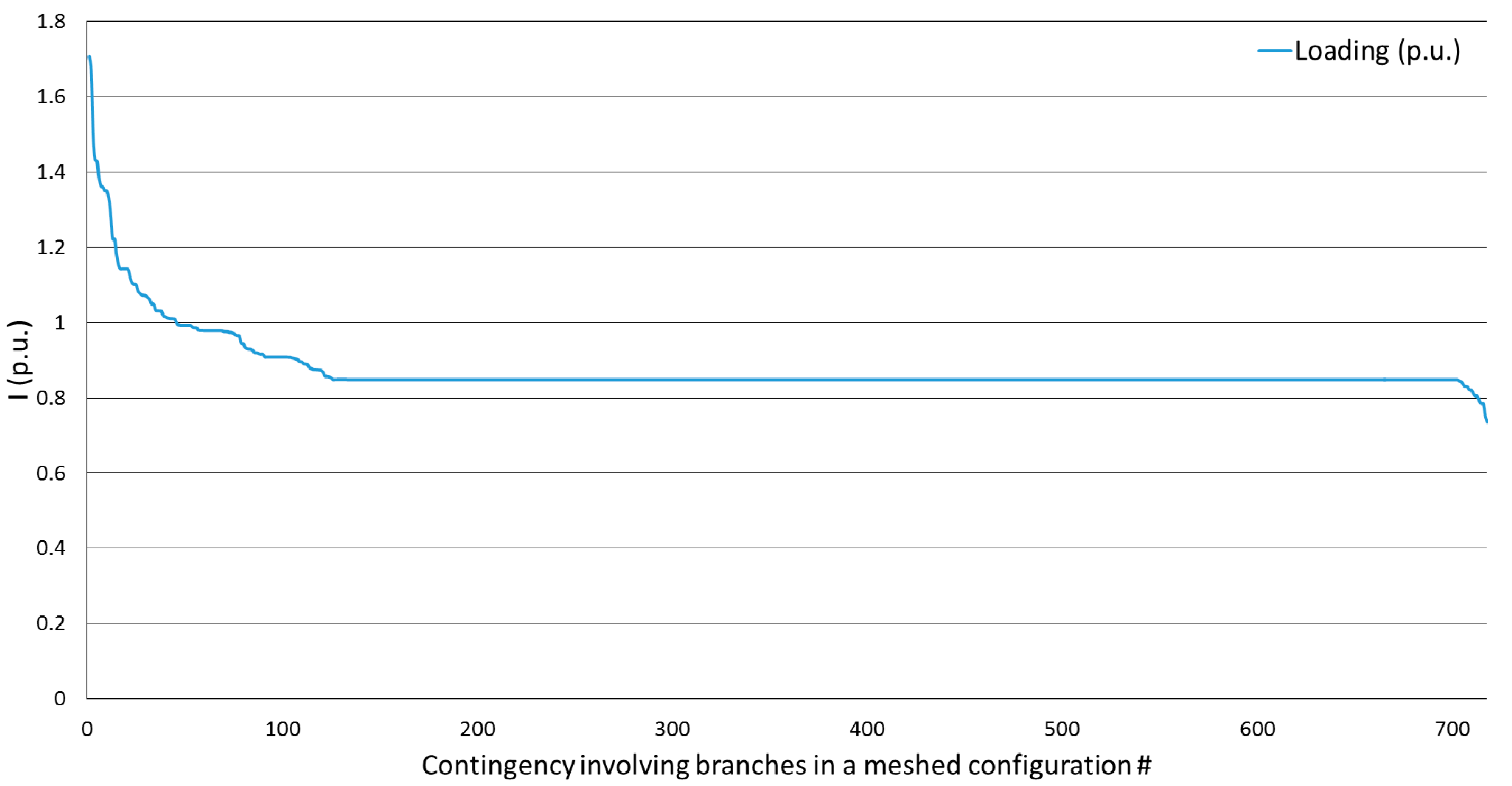
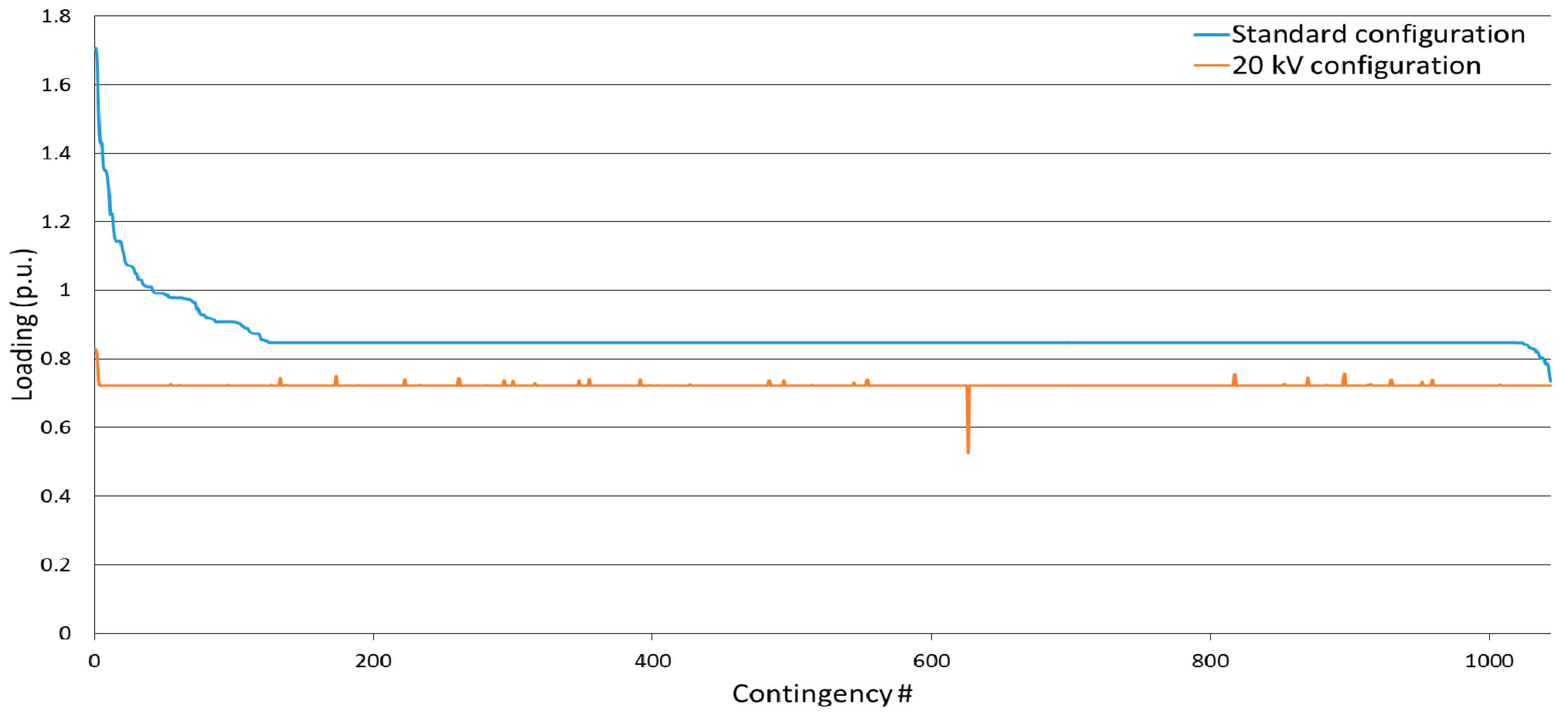
• The above-mentioned underestimation is more accentuated in portions of the distribution network with a meshed configuration, whereas it is negligible in portions of the network with branches in the antenna.
• Network reconfiguration may be ineffective both for the resilience assessment and for the choice of corrective actions improving resilience, if network constraints are not taken into account.

The use of data normally at the disposal of the distribution network operator make the proposed procedure easily implementable. Moreover, the generality of the resilience indexes and the robustness of the methodology allows application of the procedure to different threats that may occur both singularly and simultaneously.

References

1. Zio, E. Challenges in the vulnerability and risk analysis of critical infrastructures. Rel. Eng. Syst. Saf. 2016, 152, 137–150. [Google Scholar] [CrossRef]
2. Transmission and Distribution Committee of the IEEE Power & Energy Society. Guide for electric power distribution reliability indices. In IEEE Standard 1366; Transmission and Distribution Committee of the IEEE Power & Energy Society: Piscataway, MJ, USA, 2012. [Google Scholar]
3. Hosseini, S.; Barker, K.; Ramirez-Marquez, J.E. A review of definitions and measures of system resilience. Rel. Eng. Syst. Saf. 2016, 145, 47–61. [Google Scholar] [CrossRef]
4. Kwasinski, A. Quantitative model and metrics of electrical grids resilience evaluated at a power distribution level. Energies 2016, 9, 93. [Google Scholar] [CrossRef]
5. Fu, G.; Wilkinson, S.; Dawson, R.J.; Fowler, H.J.; Kilsby, C.; Panteli, M.; Mancarella, P. Integrated approach to assess the resilience of future electricity infrastructure networks to climate hazards. IEEE Syst. J. 2018, 12, 3169–3180. [Google Scholar] [CrossRef] [Green Version]
6. Kim, D.H.; Eisenberg, D.A.; Chun, Y.H.; Park, J. Network topology and resilience analysis of South Korean power grid. Phys. A Stat. Mech. Its Appl. 2017, 465, 13–24. [Google Scholar] [CrossRef] [Green Version]
7. Chanda, S.; Srivastava, A.K. Defining and enabling resiliency of electric distribution systems with multiple microgrids. IEEE Trans. Smart Grid 2016, 7, 2859–2868. [Google Scholar] [CrossRef]
8. Ouyang, M.; Duenas-Osorio, L. Time-dependent resilience assessment and improvement of urban infrastructure systems. Chaos Interdiscip. J. Nonlinear Sci. 2012, 22, 033122. [Google Scholar] [CrossRef] [PubMed] [Green Version]
9. Bessani, M.; Massignan, J.A.D.; Fanucchi, R.Z.; Camillo, M.H.M.; London, J.B.A.; Delbem, A.C.B.; Maciel, C.D. Probabilistic assessment of power distribution systems resilience under extreme weather. IEEE Syst. J. 2019, 13, 1747–1756. [Google Scholar] [CrossRef]
10. Maliszewski, P.J.; Perrings, C. Factors in the resilience of electrical power distribution infrastructures. Appl. Geogr. 2012, 32, 668–679. [Google Scholar] [CrossRef]
11. Bie, Z.; Lin, Y.; Li, G.; Li, F. Battling the extreme: A study on the power system resilience. Proc. IEEE 2017, 105, 1253–1266. [Google Scholar] [CrossRef]
12. Presidential Policy Directive—Critical Infrastructure Security and Resilience. Available online: https://www.whitehouse.gov/the-press-office/2013/02/12/presidential-policy-directive-critical-infrastructure-security-and-resil (accessed on 10 May 2021).
13. Sector Resilience Report; Office of Cyber and Infrastructure Analysis (OCIA), National Protection and Programs Directorate, Infrastructure Sector Assessment, Department of Homeland Security: Washington, DC, USA, 2014.
14. U.S. Department of Commerce; National Institute of Standards and Technology. Community Resilience Planning Guide. 2015. Available online: http://www.nist.gov/el/building_materials/resilience/guide.cfm (accessed on 10 May 2021).
15. Watson, J.P.; Guttromson, R.; Silva-Monroy, C.; Jeffers, R.; Jones, K.; Ellison, J.; Rath, C.; Gearhart, J.; Jones, D.; Corbet, T.; et al. Conceptual Framework for Developing Resilience Metrics for the Electricity, Oil, and Gas Sectors in the United States; SAND2014-18019; Sandia National Laboratory: Albuquerque, NM, USA, 2014. [Google Scholar]
16. European Network and Information Security Agency (ENISA). Measurement Frameworks and Metrics for Resilient Networks and Services: Challenges and Recommendations; ENISA: Heraklion, Greece, 2010. [Google Scholar]
17. ARERA. Available online: https://www.arera.it/it/inglese/index.htm (accessed on 10 May 2021).
18. Linee Guida Per la Presentazione Dei Piani di Lavoro Per L’incremento Della Resilienza Del Sistema Elettrico (in Italian). Available online: https://www.arera.it/allegati/docs/17/002-17dieu_alla.pdf (accessed on 10 May 2021).
19. Amicarelli, E.; Ferri, L.; De Masi, M.; Suich, A.; Valtorta, G. Assessment of the Resilience of the Electrical Distribution Grid: E-distribuzione Approach. In Proceedings of the AEIT International Conference, Bari, Italy, 3–5 October 2018. [Google Scholar]
20. Bragatto, T.; Cresta, M.; Gatta, F.M.; Geri, A.; Maccioni, M.; Paulucci, M. Assessment and Possible Solution to Increase the Resilience of Terni Distribution Grid: The Ice Sleeves Formation Threat. In Proceedings of the AEIT International Conference, Bari, Italy, 3–5 October 2018. [Google Scholar]
21. Bragatto, T.; Cortesi, F.; Cresta, M.; Gatta, F.M.; Geri, A.; Maccioni, M.; Paulucci, M. Assessment and possible solution to increase resilience: Flooding threats in Terni distribution grid. Energies 2019, 12, 744. [Google Scholar] [CrossRef] [Green Version]
22. Bragatto, T.; Cortesi, F.; Cresta, M.; Gatta, F.M.; Geri, A.; Maccioni, M.; Paulucci, M. Assessment and Possible Solution to Increase Resilience: Heat Waves in Terni Distribution Grid. In Proceedings of the AEIT International Conference, Florence, Italy, 18–20 September 2019. [Google Scholar]
23. Cresta, M.; Gatta, F.M.; Geri, A.; Maccioni, M.; Paulucci, M.; Rizzo, A. Resilience Assessment in TDE’s Distribution Grid: Risk Model for Tree Falls. In Proceedings of the AEIT International Conference, Catania, Italy, 23–25 September 2020. [Google Scholar]
24. Linkov, I.; Trump, B.D. The Science and Practice of Resilience, 1st ed.; Springer Nature Switzerland AG: Cham, Switzerland, 2019; pp. 79–101. [Google Scholar]
25. EN Std. 50341-1. Overhead Electrical Lines Exceeding AC 1 kV. General Requirements. Common Specifications; CENELEC: Brussels, Belgium, 2013. [Google Scholar]
26. EN Std. 50341-2-13. Overhead Electrical Lines Exceeding AC 1 kV. National Normative Aspects (NNA) for ITALY; CEI: Milan, Italy, 2017. [Google Scholar]
27. Gumbel, E.J. Statistics of Extremes, 1st ed.; Columbia University Press: New York, NY, USA, 1958. [Google Scholar]
28. Kew, S.F.; Philip, S.Y.; Van Oldenborgh, G.J.; Otto, F.E.L.; Vautard, R.; Van Der Schrier, G. The exceptional summer heat wave in Southern Europe 2017. Bull. Am. Meteorol. Soc. 2019, 100, 49–53. [Google Scholar] [CrossRef]
29. Province of Terni, Office of Civil Protection. Emergency Plan of the Province, Hydro Risk (In Italian). Available online: http://cms.provincia.terni.it/on-line/Home/Areetematiche/Protezionecivile/Pianidiemergenzaprovinciale/RischioIdrogeologico/articolo7447.html (accessed on 10 May 2021).
30. Authority of Tiber Basin, Hydrogeological Plan, Technical Standards (In Italian). Available online: http://www.abtevere.it/node/88 (accessed on 10 May 2021).
31. Dunn, S.; Wilkinson, S.; Alderson, D.; Fowler, H.; Galasso, C. Fragility curves for assessing the resilience of electricity networks constructed from an extensive fault database. Nat. Hazards Rev. 2018, 19, 04017019. [Google Scholar] [CrossRef] [Green Version]
32. Heinimann, H.R.; Hatfield, K. Infrastructure Resilience Assessment, Management and Governance—State and Perspectives. In Resilience and Risk: Methods and Application in Environment, Cyber and Social Domains, 1st ed.; Linkov, I., Palma-Oliveira, J.M., Eds.; Springer: Dordrecht, The Netherlands, 2017; pp. 147–187. [Google Scholar]
33. Zimmerman, R.D.; Murillo-Sanchez, C.E.; Thomas, R.J. MATPOWER: Steady-state operations, planning, and analysis tools for power systems research and education. IEEE Trans. Power Syst. 2011, 26, 12–19. [Google Scholar] [CrossRef] [Green Version]
Figure 1. Flow chart of the methodology used to evaluate vulnerability coefficients.
Energies 14 04303 g001
Figure 2. (a) Hydrogeological risk zones in Terni municipality according to [29,30] (red: Zone A; green: Zone B; yellow: Zone C; black: hydro basins); (b) SSs location in the hydrogeological risk zones (green bullets: SSs).
Energies 14 04303 g002
Figure 3. Subareas in Terni municipality according to tree fall threat.
Energies 14 04303 g003
Figure 4. Yearly load profile generated for an LV user with 3 kW contractual power.
Energies 14 04303 g004
Figure 5. Flow chart of the procedure.
Energies 14 04303 g005
Figure 6. Maximum branch loading (grey line, in per unit of the rated branch capacity), maximum bus voltage (blue line, in per unit of the rated bus voltage) and minimum bus voltage (orange line, in per unit of the rated bus voltage) caused by each contingency.
Energies 14 04303 g006
Figure 7. Number of overloaded branches due to each contingency able to cause branch overloads (contingencies are identified here by a branch id, which is the id of the branch disconnected, and correspond to the first 39 contingencies in Figure 6).
Energies 14 04303 g007
Figure 8. Number of disconnected buses in Case A simulations (in yellow) and maximum branch loading (in blue, the same trend reported in Figure 6).
Energies 14 04303 g008
Figure 9. Maximum loadings (in p.u. of the branch capacity) due to contingencies involving branches located in meshed portions of the PDN.
Energies 14 04303 g009
Figure 10. Maximum loadings (in p.u. of the branch capacity) due to contingencies involving branches in antenna.
Energies 14 04303 g010
Figure 11. Comparison between maximum branch loadings (in per unit of the branch capacity) for the PDN standard configuration (blue line) and the 20 kV configuration (orange line).
Energies 14 04303 g011