Machine Learning and GIS Approach for Electrical Load Assessment to Increase Distribution Networks Resilience

Abstract

Currently, distribution system operators (DSOs) are asked to operate distribution grids, managing the rise of the distributed generators (DGs), the rise of the load correlated to heat pump and e-mobility, etc. Nevertheless, they are asked to minimize investments in new sensors and telecommunication links and, consequently, several nodes of the grid are still not monitored and tele-controlled. At the same time, DSOs are asked to improve the network’s resilience, looking for a reduction in the frequency and impact of power outages caused by extreme weather events. The paper presents a machine learning GIS-based approach to estimate a secondary substation’s load profiles, even in those cases where monitoring sensors are not deployed. For this purpose, a large amount of data from different sources has been collected and integrated to describe secondary substation load profiles adequately. Based on real measurements of some secondary substations (medium-voltage to low-voltage interface) given by Unareti, the DSO of Milan, and georeferenced data gathered from open-source databases, unknown secondary substations load profiles are estimated. Three types of machine learning algorithms, regression tree, boosting, and random forest, as well as geographic information system (GIS) information, such as secondary substation locations, building area, types of occupants, etc., are considered to find the most effective approach.

1. Introduction

The smart grid revolution is ongoing all around the world, and advanced equipment is going to be deployed over distribution grids in order to improve the operation of the system [1]. In particular, advanced distribution management system (DMS) tools [2] are currently available, driving improvements in the efficiency, reliability, and security of the distribution grid.

Such equipment is mainly related to the medium-voltage (MV) grid, whilst just a limited number of sensors are related to the low-voltage (LV) side; this is mainly due to the cost/benefit ratio not being favorable for the latter case.

In this study, GIS tools are coupled with machine learning (ML) techniques in order to support smart grid deployment and, in particular, the idea is to have a limited number of secondary substations (MV/LV interface) provided with tele-controlled sensors and, consequently, to develop a tool capable of predicting the load profile of the unmonitored ones. A reliable load prediction, even for the unmonitored secondary substations, could allow the DSOs in a proper operation of the distribution grid, i.e., when overloads are expected, to activate corrective actions, i.e., to change the topology of the grid [3,4] or, if available, to schedule local flexibility resources [5]. Moreover, improving the power system awareness positively affects the reliability and resilience of the network in the face of outages [6,7].

Over the last few years, a significant increase in extreme natural events, such as earthquakes, hurricanes, heatwaves, and flooding, which have caused extensive and long-lasting interruptions, has been recorded [8,9]. The changed scenario has forced the power system operators, particularly the distribution system operators, to invest much effort to improve the network’s resilience, looking to reduce the frequency and impact of power outages caused by extreme weather events [10].

Generally, electricity load forecasting is divided into three categories based on the time scale: short term generally refers to forecasts from a few hours to a few days or weeks ahead; medium term is used for forecasting of a few months ahead, generally up to one year; long-term forecasts generally cover forecasts for years ahead [11]. Short-term electricity load forecasting is essential for controlling and programming electric power systems and, to date, has mainly been required by transmission companies when a self-dispatching market is in operation [12]. Medium- and long-term forecasts are also crucial for energy systems. For example, the medium-term electricity demand forecast is required for electric power system operation and scheduling [13], whereas long-term electricity demand forecasting is crucial for capacity scheduling and maintenance planning [14,15].

The approach proposed in this paper falls within medium-term forecasting. The authors of [16] present an approach to load forecasting in the medium-voltage distribution network in Portugal. The forecast method is based on a regression model and artificial neural networks (ANNs). The study was done with the time series of telemetry data of the EDP Distribution (the local DSO) and climatic records from the Portuguese Institute of Sea and Atmosphere (IPMA). The performance of the proposed methodology was evaluated using the statistical index mean absolute percentage error (MAPE). The authors of [17] study the impact of distributed generation on load forecasting. Thus, firstly they consider the impact of distributed generation on the load curve and propose a load forecasting model based on data cleaning and deep learning. Secondly, considering the data missing during communication and transmission, the K-nearest neighbors (KNN) algorithm is adopted to complete the missing data. Later, Pearson correlation coefficients are used for the correlation analysis of the input factors related to distributed generation, and the data are trained through long-short term memory in deep learning. The methodology is finally tested over several substations in Jiangsu Province, China. In [18], machine learning with an artificial neural network is used for forecasting the load at a particular hour of the day on a 33/11 kV electric power substation near Kakatiya University in Warangal, India. The authors of [19] propose a methodology that uses hourly and daily loads to predict the following year’s hourly loads and hence predict the peak loads expected to be reached in the coming year. The technique is based on implementing multivariable regression on the previous year’s hourly loads. Three regression models are investigated: the linear, the polynomial, and the exponential power. The proposed models are applied to real loads of the Jordanian power system. The same authors also propose in [20] a technique that uses hourly loads of successive years to predict hourly loads and peak load for the following selected period. The proposed method implements a new combination of some existing and well-established techniques. This is done by first filtering out the load trend, then applying the singular value decomposition (SVD) technique to de-noise the resulting signal. Hourly load is thus divided into three main components: (a) a load trend-following component, (b) a random component, and (c) a de-noised component. Results of applying the technique to the Jordanian power system showed that good forecasting accuracies are attained. Ref. [21] describes the statistical methodology of multiple linear regression (MLR) and autoregressive integrated moving average (ARIMA) methods for mid-term load forecasting. Since the monthly peak load is a nonlinear and nonstationary signal, the authors proposed a statistical methodology to solve this problem using multiple linear regression and the autoregressive integrated moving average, based on a historical series of electric peak load. The paper focuses on forecasting monthly peak load for 12 months ahead for the peak load demand of Thailand. The authors of [22] focus on forecasting short and medium terms of electrical load using three machine learning models: linear regression (LR), support vector regression (SVR), gradient boosting regression trees (GBRT). The input features contain the correlation between the weather information and the electrical load data. The proposed models are tested using the New York Independent System Operator (NYISO) dataset.

This paper presents a machine learning GIS-based approach to estimate a secondary substation’s load profiles, even in those cases where monitoring sensors are not deployed. For this purpose, a large amount of data from different sources has been collected and integrated to describe secondary substation load profiles adequately. Based on real measurements of some secondary substations given by the DSO of Milan and georeferenced data gathered from open-source databases, unknown secondary substation load profiles are estimated. Three types of machine learning algorithms are tested and compared: regression tree, boosting, and random forest. Geographic information system (GIS) information, such as the secondary substation’s location, building area, types of occupants, etc., are also used to find the most effective approach. Therefore, one of the paper’s contributions is to combine network and GIS data to improve secondary substation load profile forecasts. The remainder of the paper is organized as follows: Section 2 is devoted to introducing machine learning techniques, Section 3 details the proposed approach, Section 4 describes the real-life study case adopted to test and validate the algorithm and, in particular, a complex study case, based on the city of Milan (north of Italy), is proposed. Finally, results are reported in Section 5.

2. Machine Learning for Electrical Load Assessment

There are many types of machine learning algorithms, and typically they can be split up depending on how the machine accumulates data and information and how it learns. The two main categories are unsupervised and supervised machine learning. Even though supervised learning has been used in this study, a brief overview is also given for unsupervised learning.

2.1. Unsupervised Learning

In unsupervised learning, the machine has access only to unlabeled information and has no examples of using them. The machine itself categorizes the information available, organizes it, and learns how to utilize it to get valuable results. The goal is to extract, from the available data, structures that can describe them more straightforwardly and intuitively, such as clusters, quantiles, or general patterns.

Two of the most popular unsupervised machine learning methods are principal component analysis (PCA) and k-means clustering. PCA’s main task is to extract a low-dimensional representation of the data. It is often helpful to have a low-dimensional embedding that ideally maintains the original dataset’s relevant properties instead of many high-dimensional data [23]. Moreover, the PCA allows for obtaining efficient information representation, computation, de-noising, feature extraction, and visualization. On the other hand, k-means clustering is an unsupervised method used to divide the data into a certain number of subassemblies, usually named clusters. The aim is to collect similar samples within the same cluster, and this is also called data segmentation. Choosing the right initial points for centering the clusters and a suitable metric to define the samples’ closeness is crucial for this algorithm.

2.2. Supervised Learning

In supervised learning, the algorithm is fed with a series of codified knowledge, a sort of database with inputs and outputs that will represent the machine’s experience. The observations are called samples; every sample is composed of a certain number of features (input) and labels or targets (output). Supervised learning aims to map the inputs to obtain the correct output properly. There are different methods for this, but they can be summarized as a regularized empirical risk minimization problem that can be expressed by Equation (1).

$$mi{n}_{fϵH}\frac{1}{n}{\displaystyle \sum }_i^{n}L\left(y_i,f\left(x_i\right)\right)+\frac{\lambda }{2}\parallel f{\parallel }_H$$

(1)

where the first term is a measure of the quality of fit, in which different loss functions L can be used to compare the actual value $y_i$ with the value achieved from the model $f$ with the input variables $x_i$. The second term has the function of penalizing too complex models to avoid overfitting. Different learning problems can be formulated. Some examples of well-known supervised learning include: (i) assuming a linear function space, a squared loss function, and a squared norm regularization, we can define a linear/ridge regression; (ii) remaining in a linear function space but applying some transformation to model the conditional probability, we can achieve a logistic regression where the targets are categorical; (iii) the support vector machine has a linear classifier, which operates an extensive margin separation logic thanks to the insertion of a hinge loss that becomes larger if the fitting value is far from the actual value and penalizes the misclassification errors. Nonparametric regression, e.g., the k-nearest neighbor algorithm, is a method in which the number of model parameters grows as the amount of training data increases. The function space is made up of all the functions that have continuous second-order derivatives. Another example is the so-called decision tree, the type of supervised learning algorithm used in this study.

A decision tree uses the sum of squared loss as empirical risk minimization and a greedy heuristic logic on rectangle regions. The decision tree is a type of supervised learning mainly used for classification problems, and it is a very ductile method, working with categorical and continuous input and output variables [24]. First, the method starts dividing the samples into homogeneous sets, taking into account the features that better separate the samples. In other words, the algorithm searches for the independent variable that creates the most homogeneous differentiation of the results. The nomenclature of decision trees is as follows:

• Root: the starting point of the tree which contains all the considered samples. The root has only outgoing arrows.
• Nodes: groups of samples created by dividing the samples of a previous node. Nodes have incoming and outgoing arrows.
• Leaves: terminal nodes of the tree, where a decision is finally made. Leaves only have incoming arrows.
• Branch: a smaller tree containing only a part of the whole tree.
• Parent/child: a node is the child of the upper node and the parent of the lower node.
• Pruning: the process of removing a portion of the tree starting from the leaves. It is usually done to avoid overfitting.

The splitting process is done with a greedy approach called binary splitting. The samples are progressively split into branches from the root node. The algorithm is greedy because it looks for the feature that best divides the current samples and does not care about the future splits. The splitting process can rely on different techniques, such as Gini, information gain, chi-square, and reduction in variance [25]. One of the approaches to increase the accuracy of a tree-based algorithm is to perform an ensemble method. Ensemble techniques combine weak learners to achieve a strong learner with higher performances [26]. Ensemble methods are mainly divided into bagging and boosting.

Bagging consists of combining the results of multiple classifiers modeled on a series of subsamples generated from the same original dataset. The multiple subdatasets are created by selecting a certain number of samples randomly, and they can also be repeated. For each subdataset, a model is created, and the final prediction is made, taking into account all the responses of all the models created using a mean, a median, or a mode of them. These results are usually more robust than the original ones. Different implementations for bagging exist. The most famous is the random forest. In this case, every tree is built with a different sample of the dataset created. Moreover, to create the tree at each step, the choice of the best splitting feature is made only between a restricted number of randomly selected features, allowing the creation of more different trees.

Boosting is a method to convert weak learners into strong learners. The idea is similar to bagging: in this case, the final model will also combine the prediction of the others but using a weighted average, it tries to add new models that behave in a better way than the previous failure. The main difference from bagging, where the training stage is parallel, is that in boosting the building of learners is sequential. In other words, in bagging, every tree is independent, while in boosting, trees are built paying particular attention to the misclassified samples, and the samples’ weight is redistributed to select more “difficult” cases in the next subdatasets.

The goal of the study is to investigate machine learning techniques in order to develop a new procedure capable of predicting secondary substation load profiles and, in particular, GIS data are proposed as the data source for the artificial intelligence training, as detailed in the next section.

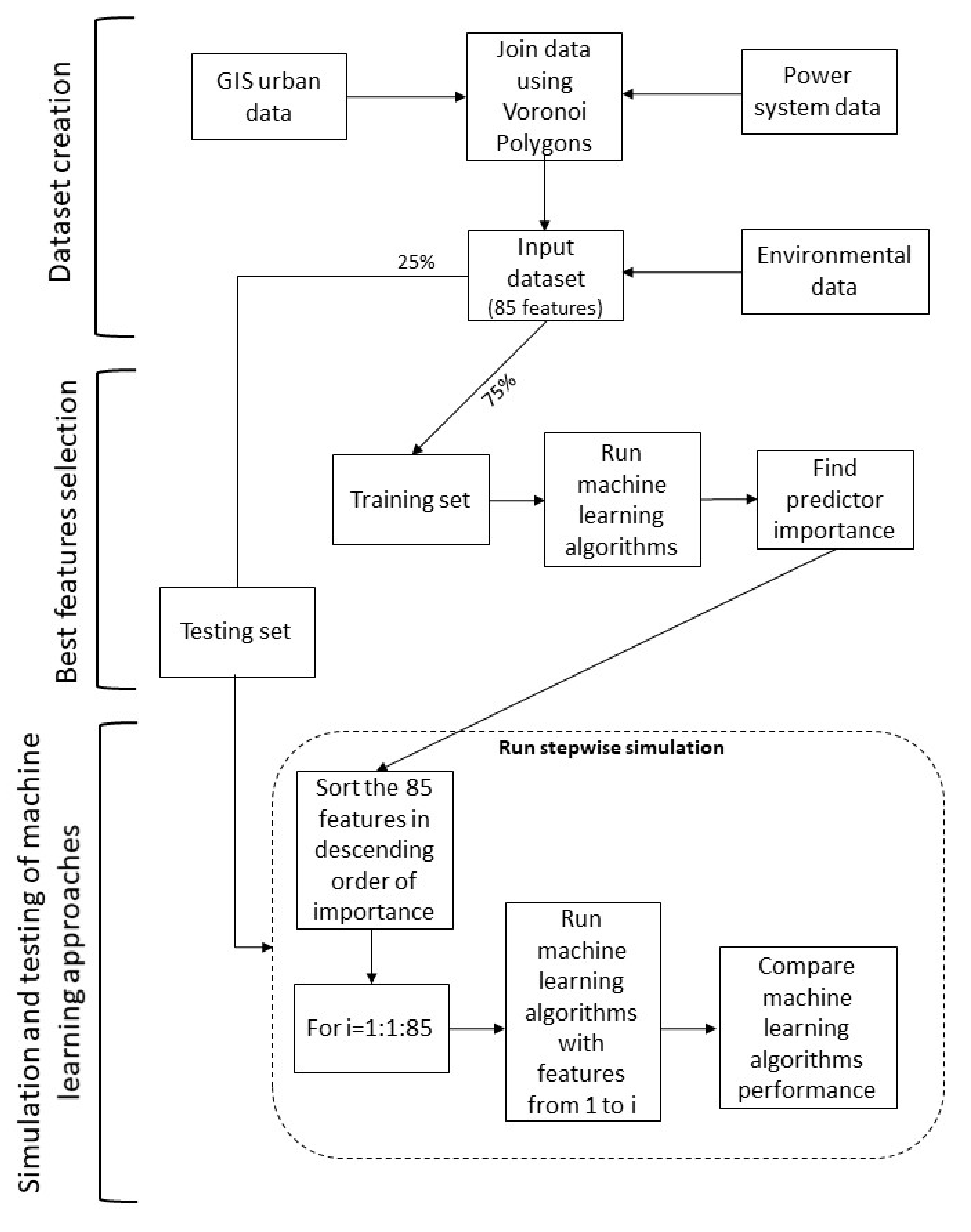
3. Proposed Approach

The study’s main objective is to propose a procedure for estimating the monthly load profile of a series of unmonitored secondary substations to improve the electrical network system’s awareness. We work on a real-life study case, thanks to the cooperation with Milan’s DSO Unareti, to properly evaluate the data complexity of a realistic scenario. We collect power system data, environmental features, and georeferenced information to improve the forecasting ability of machine learning models. The proposed approach can derive a load profile for unmonitored secondary substations based on data relevant to the monitored ones, considering load profiles and some selected characteristics. More than one model is tested, and different combinations of parameters for the same model are also explored. The models themselves are employed to extrapolate a first indication of the features’ importance as an input for the subsequent simulations. The procedure indicates which features are more important and lead to more precise predictions on load profiles and the ones that are misleading or redundant. Figure 1 shows the flowchart of the proposed approach. The procedure is based on the following steps:

• Dataset creation: we collect georeferenced and power system data, joining them to create the input dataset. Since machine learning techniques are “garbage in–garbage out” approaches, an accurate check of the data must be done at every stage of the process. A clustering using Voronoi polygons [27] is also carried out to assign the georeferenced data to the corresponding secondary substation.
• Best features selection: we consider all the available features estimating the predictor importance to gain information on which features are more promising, impacting the machine learning targets.
• Simulation and testing of machine learning approach: based on the results of the feature selection, a recursive approach is developed, which progressively adds features, testing the performances of three different machine learning approaches: regression tree, least-squares boosting, and random forest. The simulation results are collected and evaluated using different parameters to compare the machine learning methods considered.

3.1. Dataset Creation

The input dataset mainly comprises georeferenced urban environment information and power system data related to secondary substations. To match the urban information to the correspondent secondary substation, an approach that computes the service area of each secondary substation is implemented. Basically, we apply a Voronoi diagram to secondary substations to divide the city area into independent regions. The Voronoi algorithm decomposes a set of objects, secondary substations, in a spatial space into a set of polygonal partitions, the secondary substation service areas. Figure 2 shows an example of a Voronoi diagram where each secondary substation, denoted by a red circle, is placed in a separate service area. Formally, for any set of secondary substations in the two-dimensional space, a polygonal shape surrounds the object such that any point in the polygon is closer to its generated secondary substations than any other ones.

Mathematically, if we consider a metric space X, a distance function d, and a set of sites $P_k$ in the space X, the Voronoi region $R_k$, associated with the sites $P_k$, is the set of all points in X whose distances to $P_k$ are not greater than their distances to other sites $P_{j\ne k}$:

$$R_k=\left\{x\in \left.X\right|d\left(x,P_k\right)\le d{\left(x,P_j\right)}_{\forall j\ne k}\right\}$$

(2)

For the study, the distance between points is measured using the Euclidean distance:

$$d=d\left[\left(a_1,a_2\right),\left(b_1,b_2\right)\right]=\sqrt{{\left(a_1-b_1\right)}^2+{\left(a_2-b_2\right)}^2}$$

(3)

Different algorithms can be used to build a Voronoi diagram. On the one hand, there are direct ones either like Fortune’s algorithm that starts from a set of points in a plane [28] or Lloyd’s algorithm that uses a k-means clustering approach [29]; on the other hand, there are indirect methods like the Bowyer–Watson algorithm that starts from the Delaunay triangulation and then creates the Voronoi diagram [30].

Defining secondary substation service areas by just considering the geometrical distance is not always the best choice. In this study, electrical information must be taken into account, assuming that secondary substations with higher installed power probably serve larger areas. In this sense, it is more reasonable to use a weighted Voronoi diagram [31,32]. In a weighted Voronoi diagram, the cells are defined based on a geometrical distance scaled by a valuable weight. Given $n$ sites $s_1,s_2,\dots ,s_n$ and an associated weight $w_i$ for each site $s_i$, the distance from a point $p$ to a site $s_i$ is therefore defined as:

$$\mathrm{d}\left(p,s_i\right)=\frac{\left|p-s_i\right|}{w_i}$$

(4)

A weight proportional to secondary substations’ capacity to model is considered so that the one with more considerable weight will cover a more extensive area.

Finally, starting from the location of the secondary substations, we first build the weighted Voronoi diagram. Then, we join georeferenced urban environment information in the service areas with the related secondary substations to create the input dataset.

3.2. Feature Selection

Generally speaking, not all the features can be helpful in the same way. Some of them can be redundant or irrelevant. Furthermore, in machine learning applications, including these features may deteriorate their performances instead of helping to find a better solution. For these reasons, one of the most crucial steps is identifying the most valuable and informative features with so-called feature selection. The complete operation of processing the data to feed the machine learning algorithm is called feature engineering and is has two parts: the extraction and the selection.

On the one hand, extraction refers to transforming the available data to create a new smaller set of features that still captures most of the valuable information. Some algorithms can have built-in feature extraction. The primary feature extraction techniques are: principal component analysis (PCA), which creates a linear combination of the original features based on the explained variance; linear discriminant analysis (LDA), which finds a linear combination of features that characterizes or separates objects or events in classes.

On the other hand, feature selection is the filtering of irrelevant or redundant information. Feature selection choice strategies are regularly classified as the filter method, wrapper strategy, and embedded method. The filter method chooses enlightening features and stifles the least helpful to the essential model assumption. A few informativeness measurements, i.e., scores, which label the effectiveness of a feature subset, are embraced as the objective for choice purposes. The choice is made by optimizing the metric through a combinatorial search or greedy approximation. Since the definition of the metric is not bounded by a specific machine learning algorithm and is simple to compute from information, the filter strategy can be utilized for general and proficient feature selection. For instance, the features can be selected with the variance threshold principle, removing the invariable features; features that do not change much also do not add valuable information. Another way of selecting is considering the correlation of the features, keeping only one of the highly correlated features to reduce redundant information.

The wrapper strategy mixes in a learner, e.g., classifier or indicator, with the straightforward objective to minimize the classification or expectation error. In other words, a candidate feature is assessed by preparing a specific machine learning model, and the assessed generalization performance, for instance, with cross-validation, is utilized as the selection criterion. The selection strategy is typically carried out in a stagewise or greedy way to maintain a strategic distance from the combinatorial search. Thus, features chosen by the wrapper method can produce high precision for the specific learner but are not continuously appropriate for others. Other than that, the wrapper strategy becomes computationally intense when the number of candidate patterns is considerable, as the wrapped machine learning model ought to be prepared each time a feature set is assessed.

The inserted strategy implicitly chooses feature subsets by presenting sparsity within the learning model development. The main consideration is to consolidate sparsity limitations or punishments in risk minimization. However, the strategies are still model-specific, and their choice consistency is an issue in both hypotheses and honing.

In this work, three regression algorithms are considered: regression tree, least-squares boosting, and random forest. The predictor importance is evaluated with the included choice generally embedded into the algorithm, particularly by applying each of the calculations by summing changes within the mean squared error (MSE) due to parts on each indicator and dividing the entirety by the number of branch nodes. At each node, MSE is assessed as the node error weighted by the node likelihood. Variable significance related to this part is computed as the variation between MSE for the parent node and the whole MSE for the two children.

3.3. Proposed Machine Learning Approach

Based on the information on features’ importance, a modified stepwise approach is implemented. Differently from a standard stepwise search, we do not propose to train a one-feature model using each of the candidate features, keeping the one with the best performance, and then continuing to add features, one at a time, until the performance improvements stall. Instead, in our approach, we use the information taken from the predictor importance and run the models, starting with a single feature and adding features in descending order of importance. Therefore, the procedure considers the weight of the features achieved from the feature selection and sorts them from the highest to the lowest; in the first attempt, only the first features are used, and the three types of machine learning model are run; predictions are made and the monthly mean squared error is calculated on all the secondary substations in the test subset; the procedure is restarted, adding a new feature, etc. till all the features are investigated. All the simulation results are collected and evaluated with different testing subsets to find the best one and compare the different methods.

4. Input Data

This section reports the input data used by the machine learning algorithm. The datasets considered are very heterogeneous and come from multiple sources: power system data, GIS urban and environmental information. Apart from the power system data, which are the bulk information of the analysis, urban and environmental data are included to improve the forecasting ability of the machine learning models. The complete dataset consists of 3916 secondary substations; for each of them, the 85 variables included in Appendix A are available and constitute the features. At the same time, the value of the load profiles represents the label. The load profiles are the 15 min monthly trend for July 2019. Every load value represents a single sample in the dataset so that the final matrix is made up of over 6 million rows and 86 columns (corresponding to the 85 features considered and the target quantity, the load value). The 3916 secondary substations are randomly divided into the training subset, 2937, corresponding to 75%, and the testing one, 979, corresponding to 25% of the dataset.

4.1. Power System Data

Figure 3 shows the location of the 3916 secondary substations over the Milan area [33]. The density is higher near the city center and gradually decreases toward the periphery.

The following data are available for each secondary substation:

• Subscription power and number of LV customers supplied.
• Number of contracts by type: the customers are divided into 15 clusters among which 5 represent more than 95% of the power contracts.
• Number of users by type: active user, passive user, prosumer.
• Rated power and type of distributed power plants connected to the LV network, i.e., photovoltaic, hydro, thermal, biogas.

Moreover, the secondary substations are monitored, and their load profiles are stored. Data are available with 15 min resolution. An example is shown in Figure 4.

4.2. GIS Urban Data

To improve the performances of the machine learning models, we link the traditional electrical information, such as a secondary substation’s contractual power (i.e., sum of the final users’ nominal power), number of customers supplied, etc., with other environmental features to describe the urban context in which the secondary substation is located. To do this, we use QGIS software.

QGIS works with two principal data categories. The first type of data is the so-called vector layers. Vectors have a shape made up of different vertices and can represent real-world features like houses, trees, and every other thing that deserves to be indicated by the user. The vertices representing the geometry describe a position in space with latitude and longitude and, optionally, a coordinate for its height or depth. Based on the number of vertices, vector layers can be divided into a point, polyline, and polygon. The conceptual difference between the three is noticeable, but the best way to represent an object also depends on the project scale; if we consider the world map, Milan can be represented with a point but, if we consider a smaller region, it could be more appropriate to draw Milan as a polygon. Vectors can store the most disparate attributes, text, or numerical information to describe the features, such as the number of beds in a hospital or water quality in a river. The attributes can also be used as a discriminant to visualize the vector components differently. The second kind of data is called a raster, it is essentially a matrix of pixels called cells containing a value representing a characteristic of the geographic area covered by the cell [34]. Raster maps are used to visualize information that develops continuously over an area and cannot easily be divided into vectorial objects. Raster data are helpful to interpret better the vectorial quantities, putting them in the background, for example, to show a satellite picture behind a power system scheme. Raster data are commonly acquired with remote sensing by aerial photography or satellite pictures, but they can also be computed with raster analysis techniques.

The proposed approach uses georeferenced data coming from several open databases: the Milan municipality website [35]; the OpenStreetMap website, which contains maps populated by users that contribute and maintain data on roads, buildings, and facilities in general [36]; the Lombardy geoportal website [37]; the Milan geoportal website [38]; and the Italian website of open data [39] which offers information such as the location of hospitals, schools, and commercial activities, the height of buildings, number of residents, etc. From the OpenStreetMap, we collect the number of commercial activities, such as restaurants, banks, shops, and all customers that do not fall into domestic users, and we associate the related area and numbers to each secondary substation Voronoi polygon. Moreover, using data from the Milan geoportal website, we calculate the volume of the buildings. With the hypothesis that most of the buildings have a parallelepiped shape, we use a built-in QGIS function to create a volume feature from the building’s ground area and height. Details are provided in Appendix A.

Regarding domestic users, using data from the Milan municipality website, we consider every single civic number and its position and type, i.e., either residential or not residential. With a proximity analysis, these data are linked to the nearest building so that the entire building volume is also divided into residential and not residential volume. Moreover, the numbers of residential and not residential buildings are associated with each secondary substation Voronoi polygon and taken as features. Figure 5 shows the building area and residential characteristics and not residential characteristics, for a portion of the city.

We consider the so-called NIL, and the more detailed census tract map to add other features to the input dataset. As shown in Figure 6, Milan is divided into 88 quarters split into several census tracts. Supposing that the behavior of secondary substations also depends on their city location, we can add other information derived from NIL and census tracts. The census tracts do not match the Voronoi polygon perfectly, so we assign the residents to a certain Voronoi polygon proportionally to the area of census tracts that overlap it. Data on NIL and census tracts are taken from the Italian website of open data.

A similar procedure is used to assign the relative use of the ground to the secondary substation Voronoi polygon. As shown in Figure 7, using the Destinazione d’Uso del Suolo Agricolo e Forestale (DUSAF) database, it is possible to classify the city area into some classes. The first level of the database divides the surface into five main categories: anthropized areas, agricultural areas, wooded areas and semi-natural environments, wetlands, and water bodies. The other two levels go progressively deeper and define the categories more precisely: industrial, commercial, public, military, and private units; airports; arable land (annual crops); construction sites; continuous urban fabric (C.A > 80%) (covered area (C.A) is the percentage of the area covered by buildings); discontinuous dense urban fabric (C.A. = 50% ÷ 80%); discontinuous medium-density urban fabric (C.A. = 30% ÷ 50%); discontinuous low-density urban fabric (C.A. = 10% ÷ 30%); discontinuous very low-density urban fabric (C.A. < 10%); fast transit roads and associated land; forests; green urban areas; isolated structures; land without current use; mineral extraction and dumpsites; no data (clouds and shadows); other roads and associated land; pastures.

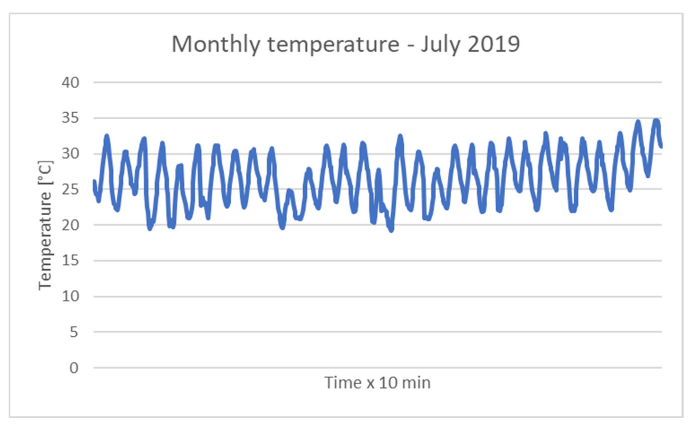
4.3. Environmental Data

Among the available environmental data, we considered the temperature. It is well known that climate is one of the critical factors influencing energy consumption [40,41]. Among various climatic factors that may affect energy consumption, temperature is the most dominant [42]. This trend is also confirmed for Milan. The use of air conditioners causes summer stress to the electrical system. Temperature records are gathered from the Regional Environmental Protection Agency (ARPA) [43]. There are several measurement stations in Milan, and we select the one located in the Brera quarter due to its barycentric position. As shown in Figure 8, the available dataset contains the average temperature with a timestamp of 10 min that is converted into 15 min data, the exact timestamp of secondary substation load profiles. Temperatures of a single day are missing. To fill the gap, we use the mean temperature of the previous and the following days.

5. Simulation Results and Discussion

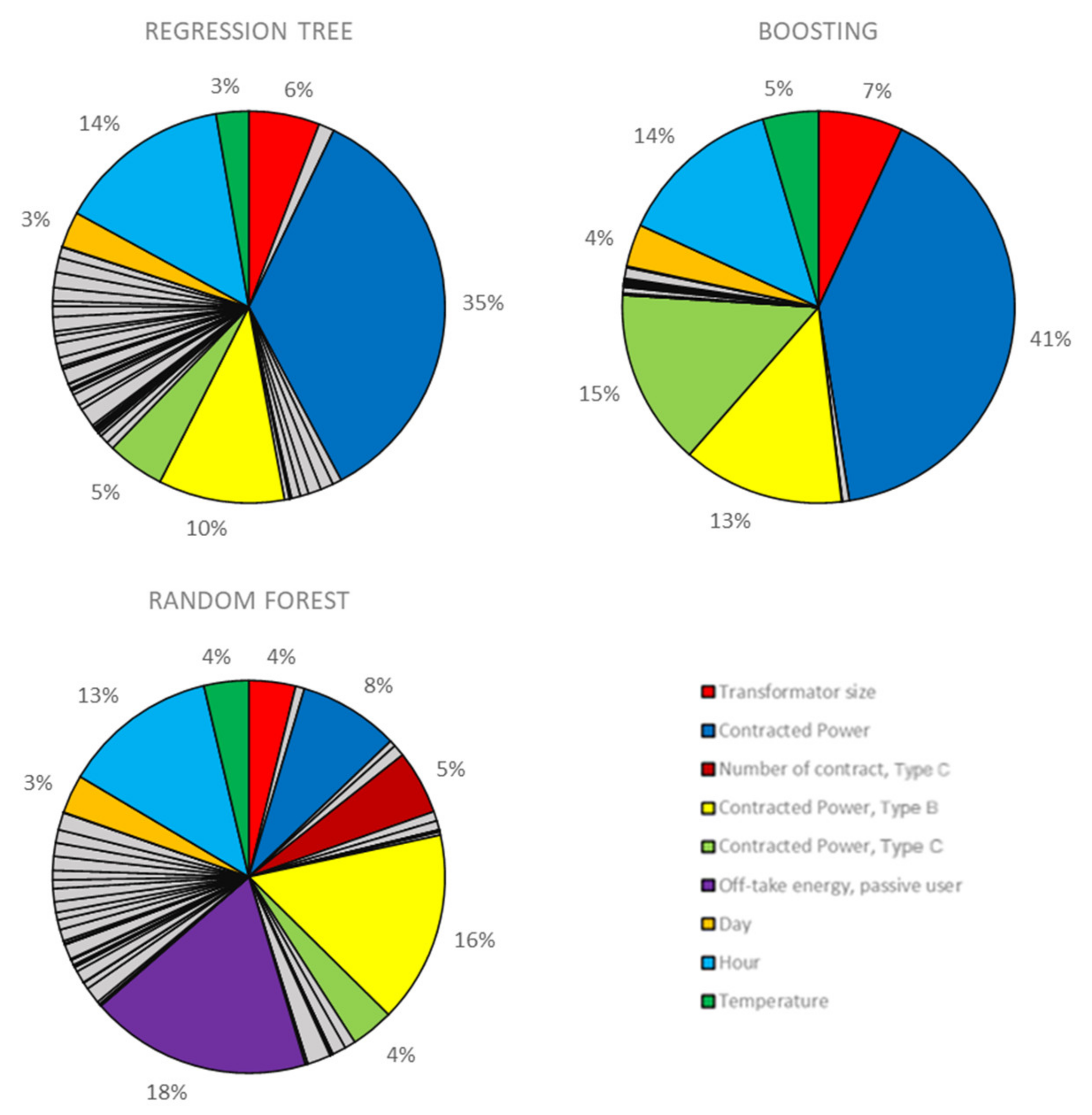
5.1. Feature Selection

With the proposed approach, 85 features are gathered in a database devoted to describing the study case; every feature is evaluated with the previously presented methodology. It is worth recalling that the final goal is to estimate the power profile of those secondary substations not provided with telecommunication equipment.

The weighted predictor importance is represented in Figure 9, where every slice represents a different predictor, and its size is proportional to its relevance. It is important to note that the result of the feature selection depends on the algorithms applied. Indeed, the proposed approach for feature selection is embedded in the machine learning algorithm.

It is possible to notice that, for each algorithm, there is a set of features that predominates the others; this behavior is particularly evident for boosting, where the sum of the relative importance of the first seven features is 96.98%, while all the other 77 features account only for the remaining 3.02%. The gap between these features and the others is less evident for the random forest. This is due to the specific algorithm that intrinsically excludes some of the features in creating the trees and therefore increases the variability of the results. Another effect of the algorithm is to highlight two more features that are less important according to the selection made by the regression tree and with boosting. These features are the number of contracts of type C and the off-take energy of passive users. Their relative importance grows while the importance of the feature “contracted power” decreases. This is because these features are strongly correlated, and the algorithm chooses the new features when the contracted power is not present in the random selection of the features for the training phase.

5.2. Stepwise Simulation

The performances of the algorithms are evaluated iteratively, repeating the training and the testing phases, each time adding one more feature. In Figure 10, the value of the monthly RMSE is represented concerning the number of features considered.

It is possible to see that all the considered methods rapidly converge to the lower errors, and each feature added after the first 8–10 causes less significant variation. The simple regression tree, after using the first predictors, starts to exhibit symptoms of overfitting. The other two methods clearly show the improvement that can be achieved considering embedded methods and, indeed, they allow a general reduction in the error. Similar RMSE values are obtained with boosting and random forest; the main difference is that the second has a trend with more oscillations, but is simultaneously the method that obtained the best absolute performances.

On each curve, the minimum monthly RMSE obtained is marked: the lower error with the boosting method is found with 7 features, with the simple tree 13 features are necessary, while with the random forest 19 features are required. In

Table 1. Features used in the best models found with stepwise analysis and their source.

Feature	R. Tree	Boosting	R. Forest	Origin
Hour	X	X	X	Intrinsic
Day	X	X	X	Intrinsic
Temperature	X	X	X	Meteo station [43]
Contracted power	X	X	X	Local DSO
Contracted power, Type C	X	X	X	Local DSO
Contracted power, Type B	X	X	X	Local DSO
Contracted power, Type E			X	Local DSO
Number of contracts, Type C	X		X	Local DSO
Number of contracts, Type B	X		X	Local DSO
Number of contracts, Type E			X	Local DSO
Number of contracts, Type D			X	Local DSO
Off-take energy, passive user			X	Local DSO
Off-take energy and release, user that can release	X		X	Local DSO
Secondary substation transformer size	X	X	X	Local DSO
Number of users connected to the secondary sub.	X		X	Local DSO
Number of activities	X		X	GIS [36]
DUSAF, area covered by other roads and associated land	X		X	GIS [37]
Census track ID			X	GIS [38]
Voronoi polygon area			X	GIS-computed
Monthly RMSE on training set [kW]	11.90	37.52	13.45
Monthly RMSE [kW]	51.53	42.91	41.73
Monthly Relative RMSE [%]	11.26	9.23	8.96

, the list of the features considered in the best solution for each of the considered methodologies is reported. Among the selected features, 12 come from the dataset of the local DSO, 4 come from the GIS information, 1 from the weather station, and 2 are intrinsic features (day and hour).

The index adopted to evaluate the performances of the three methods is the root mean square error (RMSE), computed on the quarter-hour load value of the entire month. With $N$ being the number of samples in the considered subset, $P$ the measured power, and $\widehat{P}$ the predicted one, the RMSE is computed as:

$$RMSE=\frac{1}{N}\cdot \sqrt{{\displaystyle \sum }_{month}{\left(P-\widehat{P}\right)}^2}$$

(5)

The RMSE can be computed both on the training set and the testing one. The latter is the option used to define the actual performance of the prediction. Nonetheless, it is interesting to notice that the lowest value of the RMSE computed on the training set is the one of the simple regression tree, which confirms that the algorithm is easily subject to overfitting.

The relative value of the RMSE is also computed concerning the nominal power of the transformer of the secondary substation. The relative RMSE is evaluated separately for each secondary substation of the test dataset. In Figure 11, the relative frequency of the RMSE is represented. It is possible to see that errors are lower for ensemble methods: in these cases, almost 40% of the substations have an error lower than 5%, and almost 80% have an error lower than 10%. The number of cases for which the RMSE is higher than 30% is similar in all the cases and it is always lower than 2%.

Analyzing the RMSE evaluated for working days and holidays, we see that all the models show lower errors in the forecast of the weekend load (

Table 2. Error comparison between working days and holidays.

Algorithm	Index	Working Days	Holidays
Regression tree	RMSE	52.55 kW	49.31 kW
	RMSE%	11.60%	10.51%
Boosting	RMSE	44.28 kW	39.87 kW
	RMSE%	9.54%	8.54%
Random forest	RMSE	42.65 kW	39.73 kW
	RMSE%	9.20%	8.44%

). This may be unusual because the learning algorithms should work better with more data available, but there is more information on the working days when the error is higher. On the other hand, during holidays, the load is reduced for most of the secondary substations, and the curves become more similar so the model can predict them easily. This explanation can also be confirmed by watching the error for the different days of the week (

Table 3. Error comparison among weekdays.

Algorithm	Index	Mon	Tue	Wed	Thu	Fri	Sat	Sun
Regression tree	RMSE	53.38 kW	53.06 kW	52.95 kW	51.89 kW	51.68 kW	50.34 kW	48.26 kW
	RMSE%	11.68%	11.68%	11.65%	11.46%	11.54%	10.65%	10.37%
Boosting	RMSE	44.90 kW	45.14 kW	44.94 kW	43.71 kW	42.99 kW	40.45 kW	39.28 kW
	RMSE%	9.67%	9.65%	9.61%	9.44%	9.38%	8.56%	8.52%
Random forest	RMSE	43.26 kW	43.05 kW	42.79 kW	42.17 kW	42.10 kW	40.27 kW	39.18 kW
	RMSE%	9.31%	9.26%	9.20%	9.12%	9.15%	8.51%	8.36%

). Table 3 also shows that the error on Sunday is lower than the error on Saturday for every model.

Finally, Figure 12 shows the RMSE on the test set calculated for different quarter-hours. It is possible to see that the hours that usually have the highest load also have the highest error. This behavior can be explained by the fact that at that moment of the day, the various secondary substations spread across the city present a high variability, and the models have difficulties in the proper capture of the load value. The trend of the RMSE during the day is similar for all the models, and the curves looks similar. Nonetheless, the random forest shows the best performance again because it has the lowest error in the high-load period of the day. On the contrary, the boosting method presents a lower error during the low-load period of the day.

The results obtained on the real-life case study validated the capacity of the proposed procedure to predict the secondary substations’ load profiles with sufficient accuracy. For a proper evaluation of the proposed approach, the methodology has to be correlated with the proposed implementation approach.

The procedure is used to predict load profiles for secondary substations not provided with sensors and telecommunication capabilities; in the proposed approach, such a task is performed by just relying on the power profiles of the monitored secondary substations and the GIS data of the areas fed by each MV/LV transformer. The proposed approach reported a sufficient accuracy and, on top of that, the capability to estimate the load profiles in advance, making it possible to calculate and activate possible control actions. This could be used by the DSO and could be based on an optimization of the distribution grid topology (taking into account the loading levels of the neighboring secondary substations) or in the activation of local flexibility services (currently under investigation in the Italian scenario [44]).

6. Conclusions

The study explores the possibility of predicting the power profile of MV/LV substations using machine learning approaches and GIS information. The prediction aims to increase the network’s observability and resiliency to help the sustainable growth of the electric network substation system.

Three different machine learning algorithms are applied and compared. They are all tree-based methods and include: regression tree, tree boosting, and random forest. An embedded feature selection is applied to generate a ranking of feature importance, and a stepwise analysis is proposed to identify the number of features that have to be considered to obtain the best forecast performances.

The methodology is used in a real-life case based on the distribution network of Milan. The load profiles of 3916 secondary substations with a time resolution of 15 min are provided by the local DSO, and are associated with a set of 85 features to compose the entire dataset. The features come from different origins: power system information, GIS, and weather information.

The complete dataset has an initial storage space of 4.2 GB, reduced to approximately 1 GB thanks to some data handling procedures. The three models have different computational costs based on the algorithm used and the number of features utilized; roughly, the range goes from 4 to 90 min.

Tests performed demonstrate that the ensemble methods, in particular the random forest one (RMSE = 41.73 kW, RMSE% = 8.96%), are suitable for the forecast of the secondary substation power profile. In particular, more than 90% of the evaluated substations show a relative RMSE lower than 15%.

References

1. Delfanti, M.; Falabretti, D.; Fiori, M.; Merlo, M. Smart Grid on field application in the Italian framework: The A.S.SE.M. project. Electr. Power Syst. Res. 2015, 120, 56–69. [Google Scholar] [CrossRef]
2. Berizzi, A.; Bovo, C.; Falabretti, D.; Ilea, V.; Merlo, M.; Monfredini, G.; Subasic, M.; Bigoloni, M.; Rochira, I.; Bonera, R. Architecture and functionalities of a smart Distribution Management System. In Proceedings of the 2014 16th International Conference on Harmonics and Quality of Power (ICHQP), Bucharest, Romania, 25–28 May 2014; pp. 439–443. [Google Scholar]
3. Falabretti, D.; Moncecchi, M.; Mirbagheri, M.; Bovera, F.; Fiori, M.; Merlo, M.; Delfanti, M. San Severino Marche smart grid pilot within the InteGRIDy project. Energy Procedia 2018, 155, 431–442. [Google Scholar] [CrossRef]
4. Bosisio, A.; Berizzi, A.; Morotti, A.; Pegoiani, A.; Greco, B.; Iannarelli, G. IEC 61850-based smart automation system logic to improve reliability indices in distribution networks. In Proceedings of the 2019 AEIT International Annual Conference, Florence, Italy, 18–20 September 2019. [Google Scholar]
5. Gulotta, F.; Rossi, A.; Bovera, F.; Falabretti, D.; Galliani, A.; Merlo, M.; Rancilio, G. Opening of the Italian Ancillary Service Market to Distributed Energy Resources: Preliminary Results of UVAM project. In Proceedings of the HONET 2020—IEEE 17th International Conference on Smart Communities: Improving Quality of Life using ICT, IoT and AI, Charlotte, NC, USA, 14–16 December 2020; pp. 199–203. [Google Scholar]
6. Barreto, C.; Koutsoukos, X. Design of Load Forecast Systems Resilient Against Cyber-Attacks. In Lecture Notes in Computer Science; Including Subseries Lecture Notes in Artificial Intelligence and Lecture Notes in Bioinformatics; Springer: Berlin/Heidelberg, Germany, 2019; Volume 11836, pp. 1–20. [Google Scholar]
7. Zhou, X.; Li, Y.; Barreto, C.A.; Li, J.; Volgyesi, P.; Neema, H.; Koutsoukos, X. Evaluating Resilience of Grid Load Predictions under Stealthy Adversarial Attacks. In Proceedings of the 2019 Resilience Week, RWS 2019, San Antonio, TX, USA, 4–7 November 2019; pp. 206–212. [Google Scholar]
8. Panteli, M.; Mancarella, P. The grid: Stronger, bigger, smarter? Presenting a conceptual framework of power system resilience. IEEE Power Energy Mag. 2015, 13, 58–66. [Google Scholar] [CrossRef]
9. Wang, Y.; Chen, C.; Wang, J.; Baldick, R. Research on Resilience of Power Systems under Natural Disasters—A Review. IEEE Trans. Power Syst. 2016, 31, 1604–1613. [Google Scholar] [CrossRef]
10. Panteli, M.; Trakas, D.N.; Mancarella, P.; Hatziargyriou, N.D. Power Systems Resilience Assessment: Hardening and Smart Operational Enhancement Strategies. Proc. IEEE 2017, 105, 1202–1213. [Google Scholar] [CrossRef] [Green Version]
11. Shah, I.; Iftikhar, H.; Ali, S. Modeling and Forecasting Medium-Term Electricity Consumption Using Component Estimation Technique. Forecasting 2020, 2, 163–179. [Google Scholar] [CrossRef]
12. Ahmad, A.; Javaid, N.; Mateen, A.; Awais, M.; Khan, Z.A. Short-Term load forecasting in smart grids: An intelligent modular approach. Energies 2019, 12, 164. [Google Scholar] [CrossRef] [Green Version]
13. Amjady, N.; Keynia, F. Mid-term load forecasting of power systems by a new prediction method. Energy Convers. Manag. 2008, 49, 2678–2687. [Google Scholar] [CrossRef]
14. Essallah, S.; Khedher, A. A comparative study of long-term load forecasting techniques applied to Tunisian grid case. Electr. Eng. 2019, 101, 1235–1247. [Google Scholar] [CrossRef]
15. Lindberg, K.B.; Seljom, P.; Madsen, H.; Fischer, D.; Korpås, M. Long-term electricity load forecasting: Current and future trends. Util. Policy 2019, 58, 102–119. [Google Scholar] [CrossRef]
16. Chemetova, S.; Santos, P.; Ventim-Neves, M. Load forecasting in electrical distribution grid of medium voltage. In Proceedings of the 7th IFIP WG 5.5/SOCOLNET Advanced Doctoral Conference on Computing, Electrical and Industrial Systems, DoCEIS 2016, Costa de Caparica, Portugal, 11–13 April 2016; Springer: New York, NY, USA, 2016; Volume 470, pp. 340–349. [Google Scholar]
17. Gao, Z.; Shi, J.; Li, H.; Chen, C.; Tan, J.; Liu, L. Substation Load Characteristics and Forecasting Model for Large-scale Distributed Generation Integration. In IOP Conference Series: Materials Science and Engineering; Institute of Physics Publishing: Bristol, UK, 2020; Volume 782, p. 032044. [Google Scholar]
18. Veeramsetty, V.; Deshmukh, R. Electric power load forecasting on a 33/11 kV substation using artificial neural networks. SN Appl. Sci. 2020, 2, 1–10. [Google Scholar] [CrossRef] [Green Version]
19. Abu-Shikhah, N.; Elkarmi, F. Medium-term electric load forecasting using singular value decomposition. Energy 2011, 36, 4259–4271. [Google Scholar] [CrossRef] [Green Version]
20. Abu-Shikhah, N.; Elkarmi, F.; Aloquili, O.M. Medium-Term Electric Load Forecasting Using Multivariable Linear and Non-Linear Regression. Smart Grid Renew. Energy 2011, 2, 126–135. [Google Scholar] [CrossRef] [Green Version]
21. Bunnoon, P.; Chalermyanont, K.; Limsakul, C. Mid term load forecasting of the country using statistical methodology: Case study in Thailand. In Proceedings of the 2009 International Conference on Signal Processing Systems, ICSPS 2009, Singapore, 15–17 May 2009; pp. 924–928. [Google Scholar]
22. Su, F.; Xu, Y.; Tang, X. Short-and mid-term load forecasting using machine learning models. In Proceedings of the CIEEC 2017—2017 China International Electrical and Energy Conference, Beijing, China, 25–27 October 2017; pp. 406–411. [Google Scholar]
23. Bosisio, A.; Berizzi, A.; Le, D.-D.; Bassi, F.; Giannuzzi, G. Improving DTR assessment by means of PCA applied to wind data. Electr. Power Syst. Res. 2019, 172, 193–200. [Google Scholar] [CrossRef]
24. Mosavi, A.; Salimi, M.; Ardabili, S.F.; Rabczuk, T.; Shamshirband, S.; Varkonyi-Koczy, A.R. State of the art of machine learning models in energy systems, a systematic review. Energies 2019, 12, 1301. [Google Scholar] [CrossRef] [Green Version]
25. Ringwood, J.V.; Bofelli, D.; Murray, F.T. Forecasting electricity demand on short, medium and long time scales using neural networks. J. Intell. Robot. Syst. Theory Appl. 2001, 31, 129–147. [Google Scholar] [CrossRef]
26. Zhukov, A.; Tomin, N.; Kurbatsky, V.; Sidorov, D.; Panasetsky, D.; Foley, A. Ensemble methods of classification for power systems security assessment. Appl. Comput. Inform. 2019, 15, 45–53. [Google Scholar] [CrossRef] [Green Version]
27. Bosisio, A.; Berizzi, A.; Amaldi, E.; Bovo, C.; Morotti, A.; Greco, B.; Iannarelli, G. A GIS-based approach for high-level distribution networks expansion planning in normal and contingency operation considering reliability. Electr. Power Syst. Res. 2021, 190, 106684. [Google Scholar] [CrossRef]
28. Marbate, M.P.; Gupta, M.R. Fortune’s Method: An Efficient Method For Voronoi Diagram Construction. Int. J. Adv. Res. Comput. Commun. Eng. 2013, 2, 4808–4814. [Google Scholar]
29. Reddy, D.; Jana, P.K. Initialization for K-means Clustering using Voronoi Diagram. Procedia Technol. 2012, 4, 395–400. [Google Scholar] [CrossRef] [Green Version]
30. Su, P.; Scot Drysdale, R.L. A comparison of sequential Delaunay triangulation algorithms. Comput. Geom. Theory Appl. 1997, 7, 361–385. [Google Scholar] [CrossRef] [Green Version]
31. Wang, S.; Lu, Z.; Ge, S.; Wang, C. An improved substation locating and sizing method based on the weighted voronoi diagram and the transportation model. J. Appl. Math. 2014, 2014. [Google Scholar] [CrossRef]
32. Ge, S.; Lu, Z.; Wang, C.; Wang, S. Substation planning method based on the weighted Voronoi diagram using an intelligent optimisation algorithm. IET Gener. Transm. Distrib. 2014, 8, 2173–2182. [Google Scholar] [CrossRef]
33. Bosisio, A.; Giustina, D.D.; Fratti, S.; Dede, A.; Gozzi, S. A metamodel for multi-utilities asset management. In Proceedings of the 2019 IEEE Milan PowerTech, PowerTech 2019, Milan, Italy, 23–27 June 2019. [Google Scholar]
34. Chang, K.-T. Introduction to Geographic Information Systems; Tata McGraw-Hill: New York, NY, USA, 2008; ISBN 0070658986. [Google Scholar]
35. Portale Open Data. Comune di Milano. Available online: https://dati.comune.milano.it/ (accessed on 4 June 2021).
36. OpenStreetMap. Available online: https://www.openstreetmap.org/#map=5/42.088/12.564 (accessed on 4 June 2021).
37. Home—Geoportale della Lombardia. Available online: https://www.geoportale.regione.lombardia.it/ (accessed on 4 June 2021).
38. Geoportale SIT. Comune di Milano. Available online: https://geoportale.comune.milano.it/sit/ (accessed on 4 June 2021).
39. Open Data. Sistemi Territoriali S.r.l. Available online: http://www.sister.it/sistemi-territoriali/open-data (accessed on 4 June 2021).
40. Colombo, A.F.; Etkin, D.; Karney, B.W.; Colombo, A.F.; Etkin, D.; Karney, B.W. Climate Variability and the Frequency of Extreme Temperature Events for Nine Sites across Canada: Implications for Power Usage. J. Clim. 1999, 12, 2490–2502. [Google Scholar] [CrossRef]
41. Hekkenberg, M.; Benders, R.M.J.; Moll, H.C.; Schoot Uiterkamp, A.J.M. Indications for a changing electricity demand pattern: The temperature dependence of electricity demand in the Netherlands. Energy Policy 2009, 37, 1542–1551. [Google Scholar] [CrossRef]
42. Yee Yan, Y. Climate and residential electricity consumption in Hong Kong. Energy 1998, 23, 17–20. [Google Scholar] [CrossRef]
43. Agenzia Regionale per la Protezione dell’Ambiente della Lombardia. Available online: https://www.arpalombardia.it/Pages/ARPA_Home_Page.aspx (accessed on 4 June 2021).
44. ARERA. Testo Integrato del Dispacciamento elettrico (TIDE)—Orientamenti Complessivi—Consultazione 23 Luglio 2019 322/2019/R/eel. Available online: https://www.arera.it/it/docs/19/322-19.htm# (accessed on 4 June 2021).
Figure 1. Flowchart of the proposed approach.
Energies 14 04133 g001
Figure 2. Voronoi polygons for some of the secondary substations under investigation.
Energies 14 04133 g002
Figure 3. Secondary substations’ locations within the Milan area.
Energies 14 04133 g003
Figure 4. Example of a secondary substation’s monthly load profile in p.u. of the maximum power.
Energies 14 04133 g004
Figure 5. Building area and types of occupants.
Energies 14 04133 g005
Figure 6. View of the census tracts and NIL.
Energies 14 04133 g006
Figure 7. Classification of the Milan area based on the Destinazione d’Uso del Suolo Agricolo e Forestale (DUSAF).
Energies 14 04133 g007
Figure 8. Monthly measured temperature for July 2019.
Energies 14 04133 g008
Figure 9. Relative importance of the features according to the embedded feature selections.
Energies 14 04133 g009
Figure 10. Monthly RMSE trend using features sequentially in order of importance.
Energies 14 04133 g010
Figure 11. Monthly relative RMSE for the best of each model.
Energies 14 04133 g011
Figure 12. Monthly relative RMSE for each quarter of an hour of the day.
Energies 14 04133 g012