Forecasting the Volatility of Crude Oil: The Role of Uncertainty and Spillovers

Abstract

We use a dataset for the group of G7 countries and China to study the out-of-sample predictive value of uncertainty and its international spillovers for the realized variance of crude oil (West Texas Intermediate and Brent) over the sample period from 1996Q1 to 2020Q4. Using the Lasso estimator, we found evidence that uncertainty and international spillovers had predictive value for the realized variance at intermediate (two quarters) and long (one year) forecasting horizons in several of the forecasting models that we studied. This result holds also for upside (good) and downside (bad) variance, and irrespective of whether we used a recursive or a rolling estimation window. Our results have important implications for investors and policymakers.

1. Introduction

Heightened macroeconomic uncertainty, as observed over the last decade and half due to the global financial crisis (GFC), the European sovereign debt crisis, and, of course, the ongoing COVID-19 pandemic, has tended to make the path of the future aggregate demand of commodities, and, as a result, also aggregate production, less predictable. Given this, risk averse commodity producers prefer to hold physical inventory, which causes a rise in the convenience yield, which, in turn, results in increased volatility of commodity prices, as outlined in the ‘Theory of Storage’ [1,2]. With crude oil being undoubtedly the most actively traded commodity, quite a few recent studies have analyzed the role of uncertainty in forecasting the volatility of the oil market (see, for example, [3,4,5,6,7]). For earlier studies, the reader is referred to the references cited in these papers.

As far as the existing literature is concerned, Bonaccolto et al. [3], analyzed the relevance of newspaper-based measures of economic policy and equity market uncertainty of the United States (US) in predicting the conditional quantiles of crude oil returns and volatility, using a nonparametric k-th order causality-in-quantiles model. A dynamic analysis showed that these US-based uncertainty indexes are primarily relevant during periods of market distress, when the role of oil risk is the predominant interest, with heterogeneous effects over different quantile levels.

Along similar lines, Bouri et al. [4] analyzed the predictive power of a daily newspaper-based index of US uncertainty associated with infectious diseases (EMVID) for oil-market volatility. These authors documented that incorporating EMVID into a forecasting setting significantly improved the forecast accuracy of oil volatility at short-, medium-, and long-run horizons, based on a heterogenous autoregressive model of (realized) volatility. Li et al. [5], using a mixed data sampling generalized autoregressive conditional heteroscedastic (MIDAS-GARCH) model, highlighted the role of monetary policy uncertainty in addition to overall economic policy uncertainty of the US in forecasting oil market volatility.

However, Dutta et al. [7], relying on a quantiles-based approach, showed that, unlike the overall uncertainty of the US related to policy decisions, equity market volatility of the US in general, and the same due to commodity market movements and crises, carried higher forecasting power for oil market volatility. Interestingly, while Li et al. [5] did not find a metric of global uncertainty to be important in forecasting oil market volatility, Liang et al. [6] did highlight its relevance along with the importance of the overall equity market volatility indices of the US, as the existing studies above discussed, using a standard predictive regression framework, model combination, and shrinkage approaches.

As can be observed from the concise review presented in the preceding paragraph, a general tendency of the above studies is to primarily incorporate the role of the uncertainty of the US in predicting movements of the oil market volatility, barring to some extent the work of Liang et al. [6], who considered a role of a measure of global uncertainty. While this is understandable to some extent given the dominance of the US as a major player in the global oil market (and also because the GFC originated in the US), Bahloul and Gupta [8] and Dinçer et al. [9], indicated that uncertainties of other economies within the G7 (comprising of Canada, France, Germany, Italy, Japan, the United Kingdom and the US) and China, also tend to drive oil market volatility due to the importance of their position as exporters and importers in the oil market.

In light of this, and the fact that oil is a global market, we forecast the quarterly realized variance ($RV$) of oil (West Texas Intermediate, WTI, and Brent crude) price volatility and consider not only the role of uncertainties of all the G7 countries and China but also their respective spillover of uncertainty to the rest of the world, over the period from 1996Q1 to 2020Q4. Accounting for the total amount of uncertainty spillovers of these major economies onto other countries renders it possible to better model worldwide uncertainty and its influence on global oil demand in a parsimonious manner, i.e., without incorporating the information from uncertainties of multiple other (135 to be exact, based on our data source, which we shall discuss later in detail) countries in the world.

In this regard, we were motivated by the work of Liang et al. [6], who suggested the need to look at a global measure of uncertainty (based on 22 countries, unlike 143 in our case) over and above the same of the US in predicting oil-price volatility. Following Andersen and Bollerslev [10], we captured $RV$ as the sum of squared returns over a quarter, which yielded an observable, unconditional, measure of volatility, which is otherwise a latent process. Conventionally, the time-varying volatility was modeled and the fit assessed using various GARCH models, under which the conditional variance is a deterministic function of the model parameters and past data. Alternatively, some recent papers considered stochastic volatility (SV) models, where the volatility is a latent variable that follows a stochastic process. Irrespective of whether one uses GARCH or SV models, the underlying estimate of volatility is not model-free (or unconditional) as in the case of $RV$.

One must realize that identifying factors that, in our case, happen to be the uncertainties of the G7 and their spillovers, that help to accurately forecast oil market volatility also has economic implications that are of key importance for both policymakers and investors. This is because, as shown by van Eyden et al. [11], movements in the second-moment of crude oil can predict slowdowns in worldwide economic growth.

Moreover, the recent financialization that has characterized developments in the oil market has led to the increased participation of hedge funds, pension funds, and insurance companies in the market, as per Bampinas and Panagiotidis [12], Degiannakis and Filis [13], and Bonato [14], which resulted in oil being viewed as an alternative investment in the portfolio decisions of financial institutions (especially post the GFC). Precise forecasts of oil-price volatility are of vital importance to oil traders, since volatility is a key input to investment decisions and portfolio choices [15].

To the best of our knowledge, this is the first paper to evaluate the out-of-sample forecasting power of uncertainties of the G7 and China and its spillovers for oil returns volatility. In order to account for the fact that market agents care about the level and nature of volatility, the latter making it important to distinguish between upside (“good”) and downside (“bad”) volatilities [16], we also forecast good $RV$ (the sum of daily squared positive returns only over a quarter) and bad $RV$ (the sum of daily squared negative returns only over a quarter), in addition to the overall $RV$.

Given that our data sample spans a 25 year period (1996–2020) of 100 quarterly observations, and we have 16 predictors, besides one lag of $RV$ that captures the well-known persistence of $RV$ associated with the oil market [17,18], we use, as our econometric approach, a machine-learning technique known as least absolute shrinkage and selection operator (Lasso), proposed by Tibshirani [19], which, in turn, is a regression-analysis method that performs both variable selection and regularization (i.e., the process of adding information to prevent overfitting) in order to enhance the prediction accuracy and interpretability of the resulting statistical model.

In this regard, it should be noted that the better performance of the Lasso model over forecast-combination methods in forecasting oil-market volatility has been demonstrated by Liang et al. [6] and, hence, motivates us to rely on this framework as well. Our paper, thus, adds to the already existing large literature on the forecastability of oil-returns volatility by considering the role of the uncertainties of major economies in the world and the associated spillover, where the literature can be grouped into the following broad categories, using a wide variety of models and macroeconomic, financial, behavioral, and climate pattern-related predictors (see, for example, Lux et al. [20]), Bonato et al. [21], Demirer et al. [22,23], Gkillas et al. [24], Bouri et al. [25]; Salisu et al. [26], and the references cited within these papers).

We organize the remainder of this paper as follows: In Section 2, we describe our data. In Section 3, we briefly discuss the forecasting models, along with the Lasso approach used to estimate these models. In Section 4, we present the results from our forecasting experiment. In Section 5, we conclude.

2. Data

As for crude oil prices, we used the nominal daily data derived from the US Energy Information Administration (EIA, https://www.eia.gov/dnav/pet/hist/RWTCD.htm (accessed on 1 May 2021)) for West Texas Intermediate (WTI). After computing the daily log-returns, we obtained quarterly overall, upside (“good”), and downside (“bad”) realized variances by taking the sum of the daily squared returns, positive returns only, and negative returns only over a specific quarter. As a robustness check, we also analyzed the quarterly $RV$ of the Brent crude oil returns, which, in turn, was also sourced from the US EIA (see https://www.eia.gov/dnav/pet/hist/RBRTED.htm (accessed on 1 May 2021)).

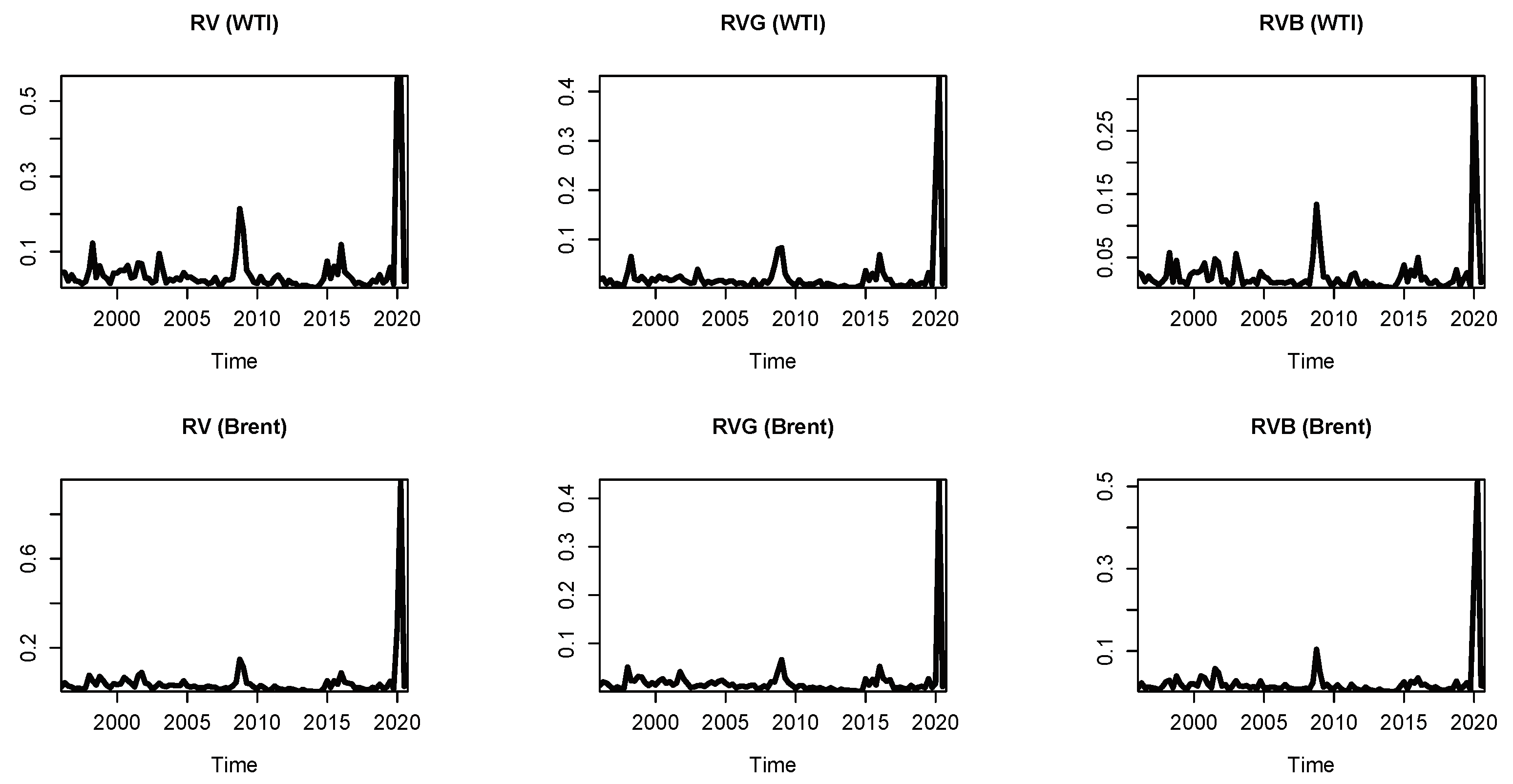
Figure 1 plots the $RV$ (and its “good” and “bad” counterparts, as defined in Section 3) of both the WTI and Brent crude oil returns. During the GFC, sharp fluctuations in RVs were observed over 2020 associated with the COVID-19 outbreak, thus, highlighting the importance of our question.

Uncertainty is a latent variable and, hence, requires methods to measure it. As documented by Gupta et al. [27], there are three broad approaches to quantify uncertainty, apart from the various ones associated with financial markets (such as implied-volatility indices, like the popular VIX, realized volatility, idiosyncratic volatility of equity returns, and corporate spreads): (1) a text-based approach, with the main idea to construct indices from searches of key words or terms related to (economic and policy) uncertainty in major newspapers or country-reports; (2) using stochastic-volatility estimates from various small and large-scale structural models (related to macroeconomics and finance) to derive measures of uncertainty; and (3) using the dispersion of professional forecaster disagreements to obtain uncertainty estimates.

For our metric of uncertainty, we used the first approach outlined by Ahir et al. [28], mainly because it is not model-specific, as it does not require any complicated estimation of a large-scale model to generate it in the first place. In addition to the uncertainty data, the associated spillover of the G7 economies and China to other economies in the world, are available publicly for download (https://worlduncertaintyindex.com/data/ (accessed on 1 May 2021)).

From frequency counts of “uncertainty” (and its variants) in the quarterly Economist Intelligence Unit (EIU) country reports from 1996 for 8 of the 143 countries, Ahir et al. [28] constructed quarterly indices of economic uncertainty for 37 countries in Africa, 22 in Asia and the Pacific, 35 in Europe, 27 in the Middle East and Central Asia, and 22 in the Western Hemisphere. The EIU reports provide an analysis and forecasts of political, policy, and economic conditions, as well as a discussion of significant political and economic developments in each country. These reports are compiled by a central EIU editorial team from work done by country-specific teams of analysts.

In order to make the uncertainty indexes comparable across countries, the raw counts were scaled by the total number of words in each report. In addition to the uncertainty indexes of each of the 143 countries, the dataset of Ahir et al. [28] also provides the uncertainty spillover metrics for the G7 and China, which, in turn, determine the choice of the countries in our paper, and the quarterly sample period of 1996Q1 to 2020Q4, which was the latest available data at the time of writing this paper. Specifically, the eight (G7 plus China) uncertainty spillover indexes of one of these particular countries to the remaining 142 countries was computed by counting the percent of word “uncertain” (or its variant) mentioned within a proximity to a word related to a particular G7 country or China in the EIU country reports.

The spillover index was then rescaled by multiplying 1,000,000 with a higher number suggesting higher uncertainty related to the specific country involving the G7 or China and vice versa. For further details regarding the words related to the G7 and China that were used, the reader is referred to Ahir et al. [28]. We used the cross-sectional sum over time to obtain the total uncertainty spillover (on to the remaining 142 economies) indexes of each of these eight countries.

Understandably, since we aimed to contribute to the oil $RV$ forecasting literature by analyzing whether accounting for spillovers of uncertainty of the G7 countries and China to the rest of the world mattered over and above the uncertainty of these economies, we relied on the method of Ahir et al. [28] for a matter of consistency and similarity in how both these indexes are derived, even though alternative ways of constructing country-level uncertainty indexes, though not spillovers, are available in the public domain (see, for example, the indexes avilable at: http://policyuncertainty.com/ (accessed on 9 July 2021) based on the work of Baker et al. [29]).

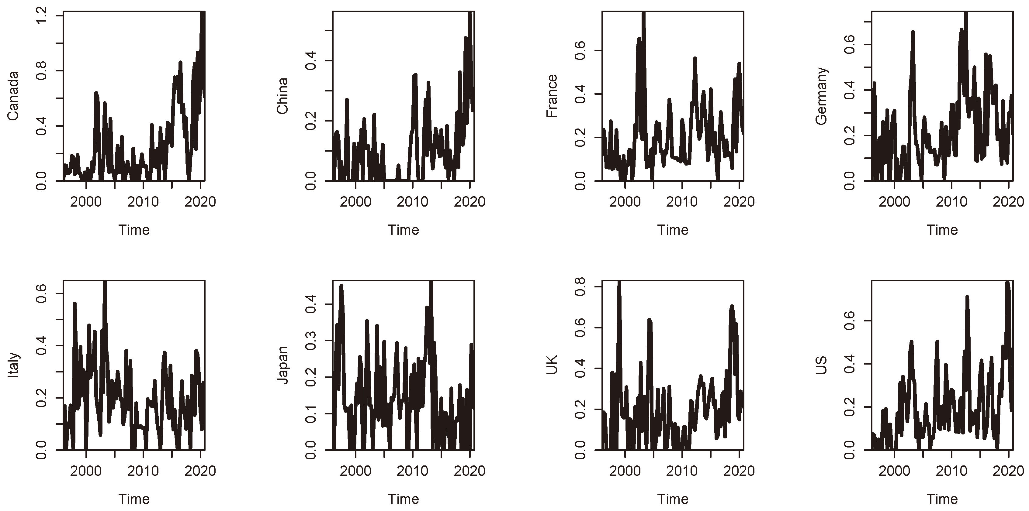
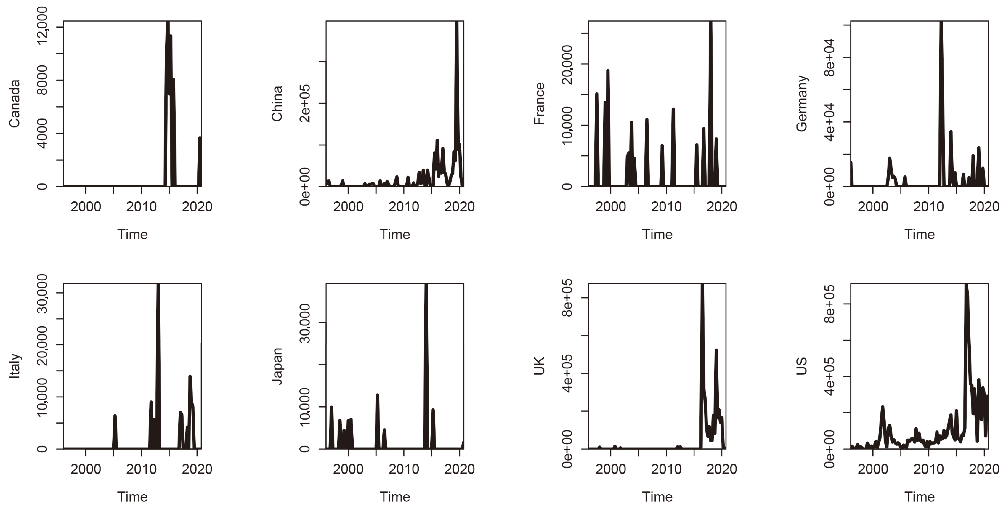
Figure 2 and Figure 3 plot the uncertainty time series and the international spillover effects. While the uncertainty series tended to fluctuate consistently over time, the spillovers had sudden massive spikes from the country(ies) of origin of the GFC, the European sovereign debt crisis, “Brexit”, and the outbreak of the Coronavirus pandemic.

3. Methodologies

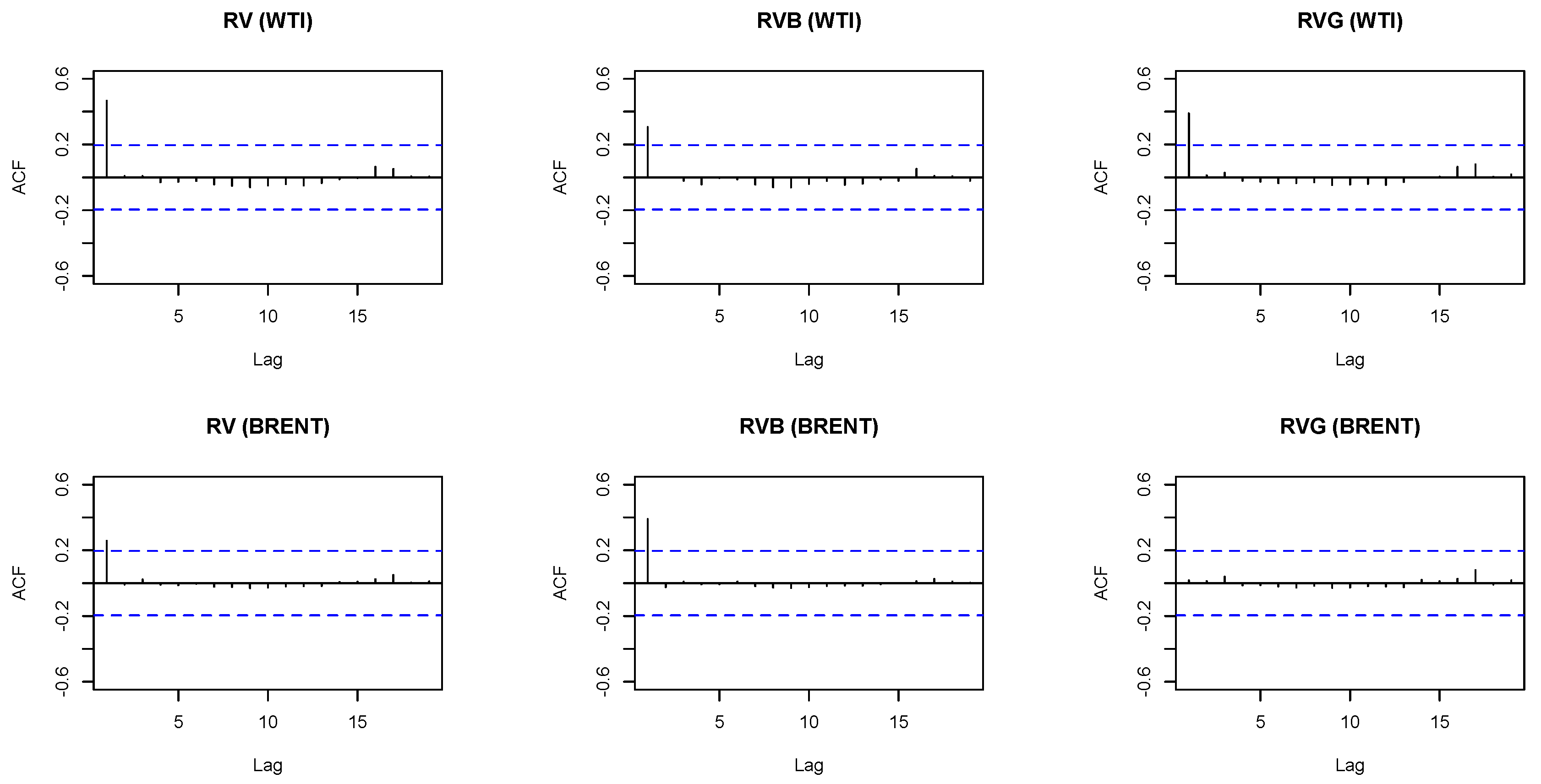
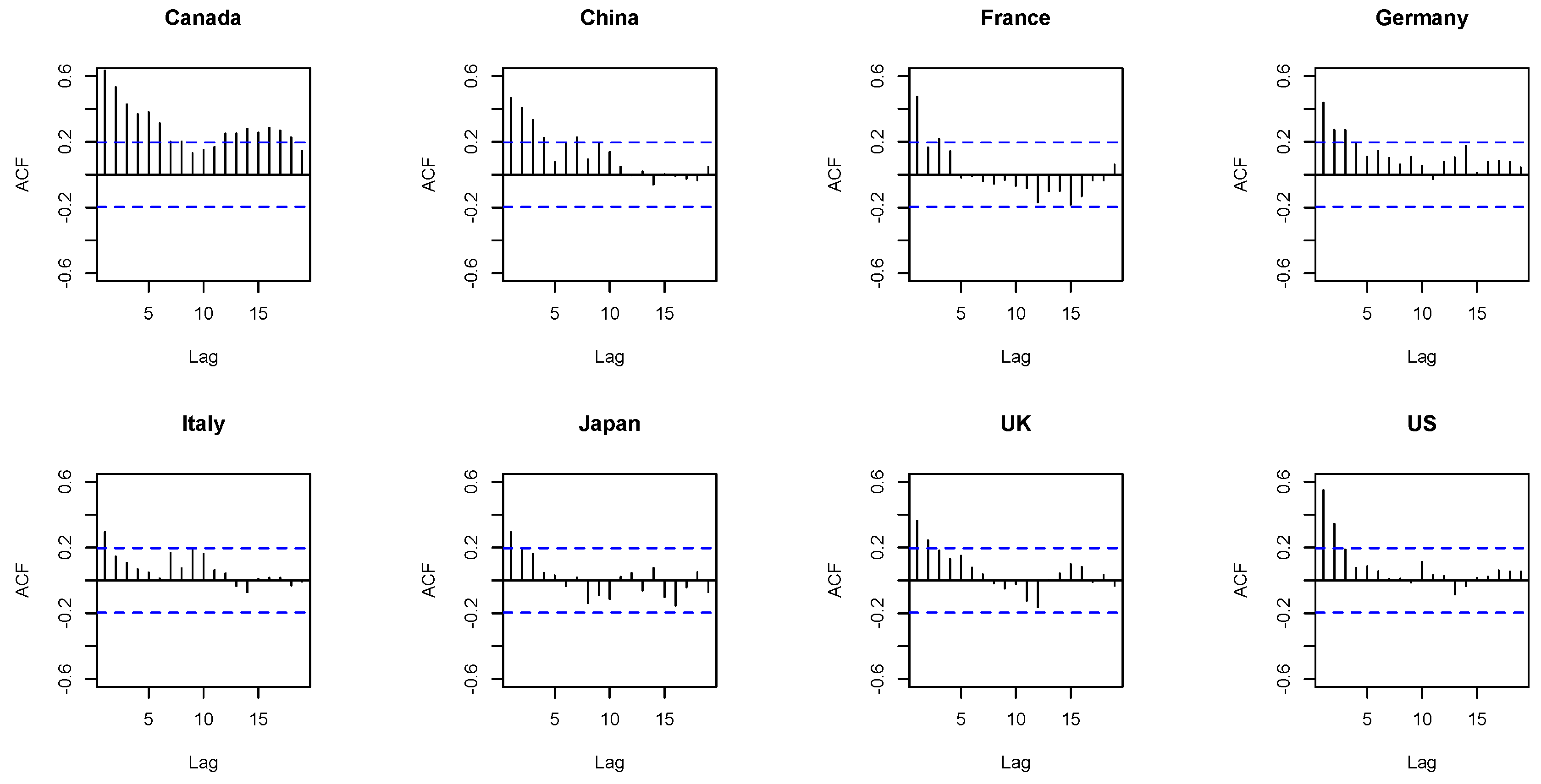
For the forecasting analysis, we used a linear regression model. The model featured an intercept and an autoregressive term as its core components. The autocorrelation functions for the realized volatility (for the estimator that we used in our empirical research, see Equations (5)) plotted in Figure 4 showed that this simple autoregressive model should suffice to capture the main elements of the persistence of $RV$ (and its “good” and “bad” counterparts).

Based on the suggestion of an anonymous referee, we also compared the in-sample performance of our benchmark autoregressive $RV$ model with that of the best-fitting GARCH model, namely the Exponential GARCH (EGARCH), in predicting $RV$ and found that the former produced a lower root mean square error (RMSEs) than the latter, which is not surprising given the insignificant coefficient in the volatility equation corresponding to the lagged GARCH term, highlighting the inability of the model to adequately capture volatility at a quarterly frequency. Complete details of these results are available upon request from the authors.

In addition, we considered the various uncertainties, U, and international spillovers, S, as additional predictors. In our empirical application, this gave four forecasting models:

$$\begin{array}{cc}\hfill R{V}_{t+h}& ={\beta }_0+\beta R{V}_t+{ϵ}_{t+h},\hfill \end{array}$$

(1)

$$\begin{array}{cc}\hfill R{V}_{t+h}& ={\beta }_0+\beta R{V}_t+\sum _{j=1}^{n_u}{\beta }_{u,j}{U}_{t,j}+{ϵ}_{t+h},\hfill \end{array}$$

(2)

$$\begin{array}{cc}\hfill R{V}_{t+h}& ={\beta }_0+\beta R{V}_t+\sum _{j=1}^{n_s}{\beta }_{s,j}{S}_{t,j}+{ϵ}_{t+h},\hfill \end{array}$$

(3)

$$\begin{array}{cc}\hfill R{V}_{t+h}& ={\beta }_0+\beta R{V}_t+\sum _{j=1}^{n_u}{\beta }_{u,j}{U}_{t,j}+\sum _{j=1}^{n_s}{\beta }_{s,j}{S}_{t,j}+{ϵ}_{t+h},\hfill \end{array}$$

(4)

where the index h denotes the forecast horizon, and (for $h>1$) $R{V}_{t+h}$ denotes the average realized variance over the forecast horizon being studied, with $h=1$, 2, and 4 in our context. When computing out-of-sample forecasts, we constructed the data matrix in such a way that the number of forecasts was the same for all forecast horizons. In addition, $n_u$ and $n_s$ denote the number of uncertainties and international spillovers being studied, and ${ϵ}_{t+h}$ denotes an error term.

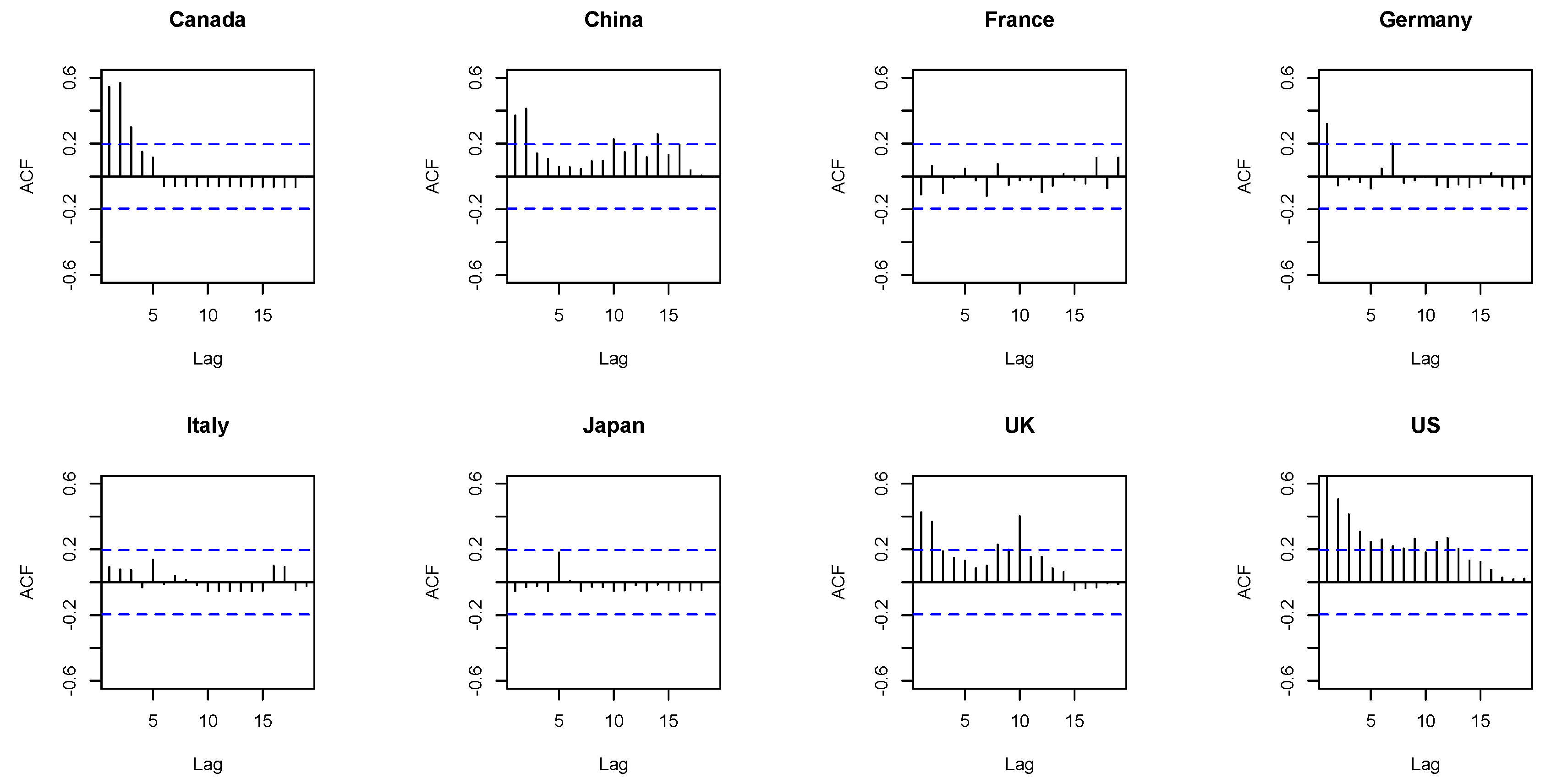
Figure 5 and Figure 6 plot the autocorrelation functions for the uncertainties and international spillovers. The figures show that all uncertainty measures exhibited a certain degree of persistence, while we observed persistence in the case of the international spillovers mainly for Canada, China, the United Kingdom, and the United States only.

As the dependent variable, we used the classical estimator of $RV$ (Andersen and Bollerslev, 1998). In our case, we used the sum of the squared daily returns per quarter. We have

$$R{V}_t=\sum _{i=1}^M{r}_{t,i}^2,$$

(5)

where $r_{t,i}$ is the daily return, which is defined as the log-difference in prices as observed on two consecutive days, and $i=1,\dots ,M$ is the number of quarterly observations. As a robustness check, we shall also study whether uncertainties and international spillovers help to forecast $\sqrt{RV}$, which researchers also often call “volatility” in empirical finance applications.

We also studied the predictive value of uncertainties and international spillovers for upward (“good”, $RVG$) and downward (“bad”, $RVB$) realized variance. Thus, we also forecast $RVG$ and $RVB$ with our forecasting equations. In line with Barndorff-Nielsen et al. (2010), we computed the bad and good realized volatility as described by the following two equations ($\mathbf{1}=$ indicator function):

$$\begin{array}{cc}\hfill RV{G}_t& {\displaystyle =\sum _{i=1}^M{r}_{t,i}^2{\mathbf{1}}_{[\left(r_{t,i}\right)>0]}},\hfill \end{array}$$

(6)

$$\begin{array}{cc}\hfill RV{B}_t& {\displaystyle =\sum _{i=1}^M{r}_{t,i}^2{\mathbf{1}}_{[\left(r_{t,i}\right)<0]}}.\hfill \end{array}$$

(7)

For the estimation of our forecasting model, we used the least absolute shrinkage and selection operator (Lasso) estimator. Our choice of the Lasso as our preferred estimation technique reflects the fact that the dimension of the forecasting model became quite large (relative to the size of our sample period) when we added the various uncertainties and international spillovers to the core components of the model. The Lasso technique chose the coefficients, $\beta ,{\beta }_{u,1},{\beta }_{u,2},\dots ,{\beta }_{s,1},{\beta }_{u,2},\dots$, so as to minimize the following expression (for a detailed discussion of the Lasso, see, e.g., Hastie et al. [30]):

$$\sum _{t=1}^N{\left(R{V}_{t+h}-{\beta }_0-\beta R{V}_t-\sum _{j=1}^{n_u}{\beta }_{u,j}{U}_{t,j}-\sum _{j=1}^{n_s}{\beta }_{s,j}{S}_{t,j}\right)}^2+\lambda \left(\left|\beta \right|+\sum _{j=1}^{n_u}|{\beta }_{u,j}|+\sum _{j=1}^{n_s}\left|{\beta }_{s,j}\right|\right),$$

(8)

where N denotes the number of observations used for estimation of the model. Hence, the Lasso shrinking used the $L1$ norm of the coefficient vectors to shrink the dimension of the estimated model. Depending on the magnitude of the shrinkage parameter, $\lambda$, the Lasso estimator shrinked and even set to zero some of the coefficients and, thus, can be viewed as a predictor-selection technique.

We selected the value of the shrinkage parameter, $\lambda$, to minimize the minimum mean cross-validated error when we used 10-fold cross validation. For estimation of the Lasso models, we used the R package “glmnet” [31]. For the R environment for statistical computing, see the R Core Team [32].

In order to compute out-of-sample forecasts, we primarily used a recursively expanding estimation window (with a training period of 10 years to initialize the estimations) and, as a robustness check, a fixed-length rolling estimation window. We, then, evaluated the forecasts by means of the Clark and West [33] test. The null hypothesis was that the models being compared had an equal out-of-sample mean-squared prediction error (MSPE).

The Clark–West test requires regressing the quantity ${\widehat{f}}_{t+h}={(R{V}_{t+h}-{\widehat{RV}}_{A,t+h})}^2-[{(R{V}_{t+h}-{\widehat{RV}}_{B,t+h})}^2-{({\widehat{RV}}_{A,t+h}-{\widehat{RV}}_{B,t+h})}^2]$ on a constant, where a hat denotes the forecast of $RV$, and the subindices A and B denote the two models under scrutiny (B denotes the larger model). The Clark–West test is based on an adjusted difference of the MSPEs implied by Models A and B. The test rejects the null hypothesis if the t-statistic of the constant in this regression model is significantly positive (one-sided test; we used Newey–West robust standard errors to study the significance of the t-statistic).

4. Empirical Results

In

Table 1. Baseline forecasting results.

Panel A: WTI
Model	h = 1	h = 2	h = 4
Uncertainty	0.8103	0.0019	0.1347
Spillovers	0.8665	0.0161	0.0681
Both	0.8930	0.0005	0.0013
Panel B: Brent
Model	h = 1	h = 2	h = 4
Uncertainty	0.1723	0.0024	0.1191
Spillovers	0.7901	0.0706	0.0463
Both	0.2008	0.0106	0.0008

CW test: p-value (based on Newey–West robust standard errors) of the Clark–West test. Training period used to initialize the recursive-estimation scheme: 40 quarters.

, we report the baseline forecasting results for WTI and Brent. The table gives the p-values of the Clark–West test. The key message to take home from the results given in the table is that the Lasso model that included uncertainty and/or international spillovers outperformed in our out-of-sample forecasting exercise for the core model at the intermediate and long forecasting horizon. We obtained this key result for both WTI and Brent crude oil-price realized variances.

We used robust standard errors to compute the p-values because (as one would have expected) the forecast errors were autocorrelated at the longer forecast horizons due to the overlapping forecast horizons. As suggested by an anonymous reviewer, we also tested whether the forecast errors had a unit root. A standard unit root test (Kwiatowski et al. [34] showed that the forecast errors could be regarded as stationary time series. Detailed results are not reported to save journal space but are available from the authors upon request.

There was also evidence of predictive value when we further extended the forecast horizon to six and eight quarters. Further, when we studied the natural logarithm of $RV$, we observed improvements in the forecasting performance at the longer and, depending on the model specification, at the intermediate forecasting horizon. Detailed results are available from the authors upon request.

In order to shed further light on the relative forecasting performance of the model, we document in

Table 2. Forecasting gains.

Panel A: WTI
Model	h = 1	h = 2	h = 4
Uncertainty	−2.2952	−0.0290	0.2379
Spillovers	−3.3006	3.0384	2.4165
Both	−2.6771	3.6453	4.4951
Panel B: Brent
Model	h = 1	h = 2	h = 4
Uncertainty	0.3186	0.6375	0.1207
Spillovers	−7.5552	−12.9077	0.3586
Both	−0.0492	1.5670	6.7234

Note: The forecasting gains are defined as $100\times ({\mathrm{RMSFE}}_0/{\mathrm{RMSFE}}_1-1)$, where the index 0 denotes the benchmark (autoregressive) model, and the index 1 denotes the alternative models (including uncertainty and/or spillovers). RMSFE: root-mean-squared-forecasting error. Training period used to initialize the recursive-estimation scheme: 40 quarters.

, for both WTI and Brent, the forecasting gains expressed as the percentage increase (or decrease) in the ratio of the root-mean-squared-forecasting error (RMSFE) of the benchmark (that is, autoregressive) model and the alternative models. A positive forecasting gain, thus, shows that the RMSFE of the benchmark model exceeded the RFMSFE of the alternative model, implying that the alternative model yielded better forecasts under a standard quadratic loss function.

We observed positive forecasting gains mainly at the intermediate and especially at the long forecasting horizon. The forecasting gains were the largest when we combined uncertainty and international spillovers ($h=2,4$). The autoregressive benchmark model, in turn, tended to fare better than the alternative models at the short forecasting horizon. Taken together, the results corroborated the results of the Clark–West test. The correlation between the forecasting gains reported in Table 2 and the p-values of the Clark–West test given in Table 1 was significantly negative (coefficient of correlation = −0.48, t-statistic of −2.19, p-value = 0.04), showing that higher forecasting gains tended to be associated with lower p-values and, thus, significant test results.

A major exception arose in the case of Brent and the spillovers model and $h=2$, where the forecasting gain was negative (and large in absolute terms), while the Clark–West test (which is, as described in the methodology in Section 3, based on the adjusted difference of the out-of-sample MSPEs generated by the two models being compared) yielded a significant result.

Next, we summarize in

Table 3. Forecasting results for upside and downside volatility.

Panel A: Bad Realized Variance (WTI)
Model	h = 1	h = 2	h = 4
Uncertainty	0.1540	0.0447	0.0334
Spillovers	0.7545	0.0362	0.4446
Both	0.9393	0.0228	0.1652
Panel B: Bad Realized Variance (Brent)
Model	h = 1	h = 2	h = 4
Uncertainty	0.4946	0.0003	0.0073
Spillovers	0.2806	0.0838	0.0472
Both	0.2907	0.0029	0.0211
Panel C: Good Realized Variance (WTI)
Model	h = 1	h = 2	h = 4
Uncertainty	0.7907	0.1301	0.5917
Spillovers	0.8808	0.0202	0.0007
Both	0.8691	0.0021	0.0003
Panel D: Good Realized Variance (Brent)
Model	h = 1	h = 2	h = 4
Uncertainty	0.6569	0.1818	0.0001
Spillovers	0.3599	0.8717	0.0027
Both	0.7035	0.4739	0.0010

Note: CW test: p-value (based on Newey–West robust standard errors) of the Clark–West test. Training period used to initialize the recursive-estimation scheme: 40 quarters.

the results (Clark–West test) for the good and bad realized variances, again for both WTI and Brent. The results corroborated that uncertainty and/or international spillovers added to the forecasting performance of the model estimated on data for bad realized variance at the intermediate and long forecast horizon. For good realized variance, we observed insignificant test results in the case of uncertainty for WTI and significant test results for international spillovers at the intermediate and long forecast horizon. In addition, the test results for both uncertainty and international spillovers were insignificant at the short and the intermediate, but not at the long, forecast horizons for Brent.

Table 4. Forecasting results for the realized volatility ($\sqrt{RV}$).

Panel A: WTI
Model	h = 1	h = 2	h = 4
Uncertainty	0.7271	0.2133	0.0255
Spillovers	0.8681	0.1204	0.1304
Both	0.8946	0.1175	0.0298
Panel B: Brent
Model	h = 1	h = 2	h = 4
Uncertainty	0.1570	0.0317	0.0083
Spillovers	0.5702	0.1058	0.0557
Both	0.4063	0.0651	0.0070

Note: CW test: p-value (based on Newey–West robust standard errors) of the Clark–West test. Training period used to initialize the recursive-estimation scheme: 40 quarters.

gives the forecasting results for $\sqrt{RV}$. We use the terms “realized volatility” and “realized variance” interchangeably in this paper, while researchers in the empirical-finance literature often use the term “volatility” to refer to $\sqrt{RV}$. The results for WTI showed that uncertainty had predictive value at the long forecast horizon, but international spillovers did not add to the forecasting performance of the model. The test results for Brent, in turn, were significant for uncertainty at the intermediate and the long forecast horizon, and for international spillovers at the long forecast horizon.

Table 5. Forecasting results for a rolling-estimation window.

Panel A: WTI
Model	h = 1	h = 2	h = 4
Uncertainty	0.0894	0.0916	0.0018
Spillovers	0.1562	0.2739	0.0775
Both	0.1395	0.1714	0.0006
Panel B: Brent
Model	h = 1	h = 2	h = 4
Uncertainty	0.1832	0.1606	0.0734
Spillovers	0.3552	0.0105	0.0020
Both	0.4020	0.0114	0.0004

Note: CW test: p-value (based on Newey–West robust standard errors) of the Clark–West test. Length of the rolling-estimation window: 40 quarters.

summarizes the results for a rolling-estimation window. The test results were significant for all three forecasting horizons (at the 10% level) for uncertainty in the case of WTI. In addition, the test results for international spillovers were significant for WTI when we studied the long forecast horizon. As for Brent, the test results for uncertainty and international spillovers were significant for the long forecast horizon and, in addition, for the intermediate forecast horizon in the case of international spillovers.

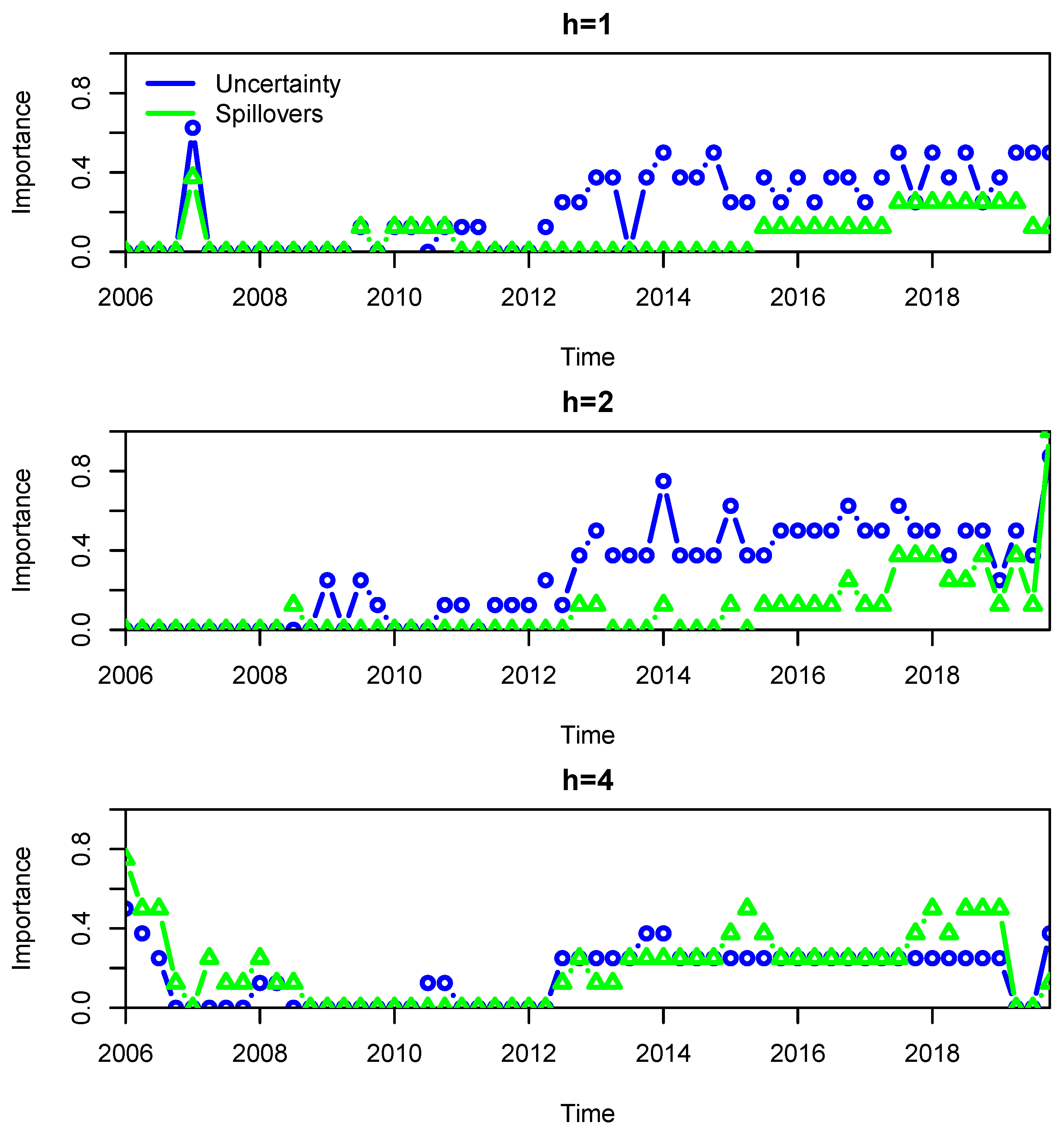
In order to illustrate how the Lasso estimator works, we plot in Figure 7 the importance of the uncertainty and international spillovers over time. The results are for WTI and a recursive-estimation window. We used a simple metric of importance. Specifically, we define importance as the number of nonzero coefficients estimated for uncertainty (international spillovers) divided by $n_u$ ($n_s$). Hence, zero means that the Lasso sets all coefficients, for example, of uncertainty to zero in a given forecasting period, and one means that all coefficients of uncertainty are included in the model.

The results show that uncertainty tended to be of more importance on average than international spillovers at the short and the intermediate forecast horizon, while the importance of both categories of predictors was more or less balanced at the long forecast horizon. The results also illustrate that the importance of both uncertainty and international spillovers was not stable over the out-of-sample period, lending support to our decision to use a recursive- and a rolling-estimation window to analyze the forecasting properties of uncertainty and international spillovers for the realized volatility over time.

This result is not surprising but is indicative of the fact that uncertainty and its spillovers themselves are not constant and vary across time (as shown in Figure 2 and Figure 3) depending on events that affect the macroeconomic uncertainty in these major economies and the associated spillovers, thereafter, to the rest of the world.

Table 6. Forecasting results for a ridge regression.

Panel A: WTI
Model	h = 1	h = 2	h = 4
Uncertainty	0.7883	0.0017	0.0005
Spillovers	0.8775	0.4673	0.1202
Both	0.8018	0.4647	0.0225
Panel B: Brent
Model	h = 1	h = 2	h = 4
Uncertainty	0.4852	0.0013	0.0027
Spillovers	0.8576	0.1443	0.0076
Both	0.8233	0.3856	0.0053

Note: CW test: p-value (based on Newey–West robust standard errors) of the Clark–West test. Length of the recursive-estimation window: 40 quarters.

summarizes, as a further robustness check, the results for a ridge-regression approach. A ridge regression also solves the minimization problem given in Equation (8) for the Lasso with the difference being that the penalty term multiplied by the $\lambda$ coefficient used the L2 norm to shrink the estimated coefficients of the forecasting model. The results show that, at the intermediate forecast horizon, only the uncertainty improved the forecasting performance, whereas, for the long forecasting horizon, both uncertainty and international spillovers (Brent) helped to improve the forecast accuracy.

Our forecasting analysis confirmed the initial premise of our paper that the uncertainties of other important economies within the G7 in addition to the US and China also tend to drive oil market volatility due to the importance of their position as exporters and importers in the oil market. Especially in the longer-run, the spillovers of uncertainty from these major economies to other countries in the world are important in capturing the accurate size of the global demand in the oil market in the wake of increased uncertainty.

The relatively stronger long-run influence of spillovers on oil market volatility is understandable, since it takes time for uncertainty originating in the G7 and China to spread to the rest of the world, via various channels namely, trade, financial markets, and exchange rates [35,36], to the extent that it leads to uncertainty convergence over time [37]. In sum, our findings are indicative of the fact that accounting for the total amount of uncertainty spillovers of the major economies, over and above their own uncertainties, allowed us to better model worldwide uncertainty and its influence on global oil demand, which, in turn, translated into more accurate forecasting of the realized variance capturing oil-market volatility.

5. Conclusions

Based on a dataset for the G7 countries and China, our results showed that uncertainty and international spillovers had predictive value in an the out-of-sample forecasting exercise for the realized variance of crude oil (West Texas Intermediate and Brent), where our sample period ranged from 1996Q1 to 2020Q4. Given that, on the one hand, our sample period was relatively short and, on the other hand, our data comprised measures of uncertainty for eight countries and eight measures of international spillovers, we used the Lasso estimator to estimate our forecasting models. Taken together, our empirical results demonstrated that, depending on the model specification, uncertainty and international spillovers had predictive value for the realized variance (and its “good” and “bad” counterparts) at an intermediate (two quarters) and a long (one year) forecasting horizon.

Compared to the current literature, which has relied only on the role of US uncertainty in predicting oil market volatility, our paper extends this line of research by highlighting the importance of not only the uncertainty of the G7 countries and China but also their respective spillovers of uncertainty to the rest of the world. This being the first study of its kind, it is impossible to provide comparative quantitative assessment of our results with the existing papers in this related area; however, its academic value in terms of depicting the pertinent role of uncertainty and its spillovers beyond the US in forecasting oil-market volatility cannot be overlooked.

In addition, our results can be used by policy authorities to obtain information on the future path of the volatility of oil prices due to uncertainty of G7 countries and China, as well as the associated global spillovers of uncertainty from these economies. This knowledge, in turn, could be useful to predict economic activity, given that oil-price volatility is known to lead business cycles. Our results, therefore, may help policymakers to reach appropriate policy decisions in the wake of the movements in the uncertainties of major global economies and the spillovers. Moreover, with volatility being a key input in portfolio decisions, the forecastability of oil-price volatility due to the uncertainties of G7 and China, as well as the associated spillovers, should be of vital importance to traders in the oil market.

Having indicated the important implications of our results, it is also necessary to acknowledge one limitation of our study in terms of the low-frequency of our data. Ideally, we would have preferred to have conducted the forecasting exercise of realized variance of oil at a higher frequency, as it is of great importance for policymakers and investors to make timely policy and portfolio decisions; however, the uncertainty spillover indexes were available only at a quarterly frequency and, hence, constrained us in our ability to provide higher-frequency (say, for example, daily or monthly) results.

As a part of future research, it would be interesting to extend our analysis to other commodity markets, in particular gold, which is a well-established safe haven in the wake of heightened uncertainty [38,39].