Control Strategy Based on Arm-Level Control for Output and Circulating Current of MMC in Stationary Reference Frame

Abstract

This paper proposed a control method for output and circulating currents of modular multilevel converter (MMC). The output and circulating current are controlled with the help of arm currents, which contain DC, fundamental frequency, and double frequency components. The arm current is transformed into a stationary reference frame (SRF) to isolate the DC and AC components. The AC component is controlled with a conventional proportional resonant (PR) controller, while the DC component is controlled by a proportional controller. The effective control of the upper arm and lower arm ultimately controls the output current so that it delivers the required power to the grid and circulating current in such a way that the second harmonic component is completely vanished leaving behind only the DC component. Comparative results of leg-level control based on PR controller are included in the paper to show the effectiveness of the proposed control scheme. A three-phase, five-level MMC is developed in MATLAB/Simulink to verify the effectiveness of the proposed control method.

1. Introduction

Recently, MMC has gained significant attention due to its use in high voltage direct current (HVDC) transmission systems [1], traction power supplies [2], static synchronous compensators (STATCOMs) [3,4], medium voltage drives [5,6,7], and offshore wind energy system [8]. The use of MMC in such a wide domain became possible due to its attractive property of scalability in terms of voltage levels, modularity, low harmonic distortion, low stress on devices, and high efficiency [1,2,3,4,5,6,7,8,9]. Besides these attractive features, MMC also faces some challenges. One of them is the flow of large magnitude circulating current in its phase legs. Circulating current is a negative sequence with a double frequency, which has no effect on the output current of MMC. However, an unsuppressed circulating current will result in a high RMS arm current and will eventually cause power loss and put additional stress on the devices. The second is the regulation of submodule (SM) capacitor voltage, which is mandatory for the stable operation of MMC. The control of output current is also important to ensure the proper delivery of active and reactive power.

In the literature, various control strategies have been proposed to overcome these challenges. The cascaded control scheme proposed by Hagiwara and Akagi [10] is mostly adopted. This control scheme is the interconnection of several control loops with phase-shifted pulse width modulation (PS-PWM) to control output current, circulating current, and capacitor voltage of MMC. However, the second harmonic component in the circulating current is not suppressed efficiently. Synchronous reference frame based $dq$ control is proposed in [11] using proportional-integral (PI) regulators. Although PI regulator provides high gain at zero frequency, interconversion between different frames increases the computational burden and small error in the transformation between frames, which can lead to large error. In [12], the authors proposed a PR controller for the control of circulating and output current. For circulating current, a multi-resonant controller is used for second harmonics suppression. However, the leg-level control results in a slow response and a high settling time. Apart from these controllers, different model predictive control (MPC) approaches are also adopted for controlling MMC in [13,14,15,16,17,18]. Nowadays, MPC is highly adopted in power converter control, but the computational burden and complex mathematical calculation of conventional MPC may not always be practical. Different approaches of sliding mode control (SMC) are discussed in [19,20], which use different loops for controlling output and circulating current. The SMC is normally subjected to chattering issues.

A feedback linearization technique is applied to MMC in [21]; after linearizing the plant, conventional controllers are used. Although after linearization, controller design and tuning become easy, mathematical derivation and implementation are not trivial. Backstepping algorithm [22], adaptive controllers [23], optimization-based control [24], and repetitive controllers [25] are proposed for controlling the parameters of MMC, specifically circulating current. The control strategies in previous work are mostly composed of two different loops for controlling circulating and output currents of MMC. The tuning of the different controllers for both loops is a laborious task. Moreover, few researchers have worked on arm-level control of MMC. In [26,27], the authors have proposed a control strategy based on arm current control. The control is carried out in a synchronous reference frame, which involves different frame transformations that increase the computation burden.

In this paper, we have proposed a control method for controlling the circulating and output current of MMC. This novel control scheme is based on arm current control. The upper and lower arm currents are independently controlled, which will assure the control of output current and suppression of circulating current harmonics by choosing a proper reference. The controller used in the upper arm and lower arm has the same characteristics. It makes the tuning of the controller easy. The same tuning parameters can be used for the upper arm controller and lower arm controller.

In order to achieve the control goal, the arm currents are transformed into SRF and decomposed into $\alpha \beta \gamma$ components. Due to the presence of fundamental frequency and second harmonic component, the $\alpha \beta$-components are controlled by a proportional resonant controller tuned at those frequencies, while the $\gamma$-component is controlled through a proportional controller. Moreover, the capacitor voltage of MMC is regulated with the help of a conventional sorting algorithm. The proposed control scheme is compared with the leg-level control scheme to show its effectiveness. The promising results of the proposed strategy show that the controller’s settling time is low due to its fast response, and the circulating current is effectively controlled to eliminate the AC components, only leaving behind the desired DC component.

The rest of the paper is organized as follows. In Section 2, the configuration, operation, and mathematical model of the system are given in detail. Section 3 sums up the designed control. The results are discussed in Section 4. The conclusion of our work is presented in Section 5.

2. MMC Configuration, Operation, and Modeling

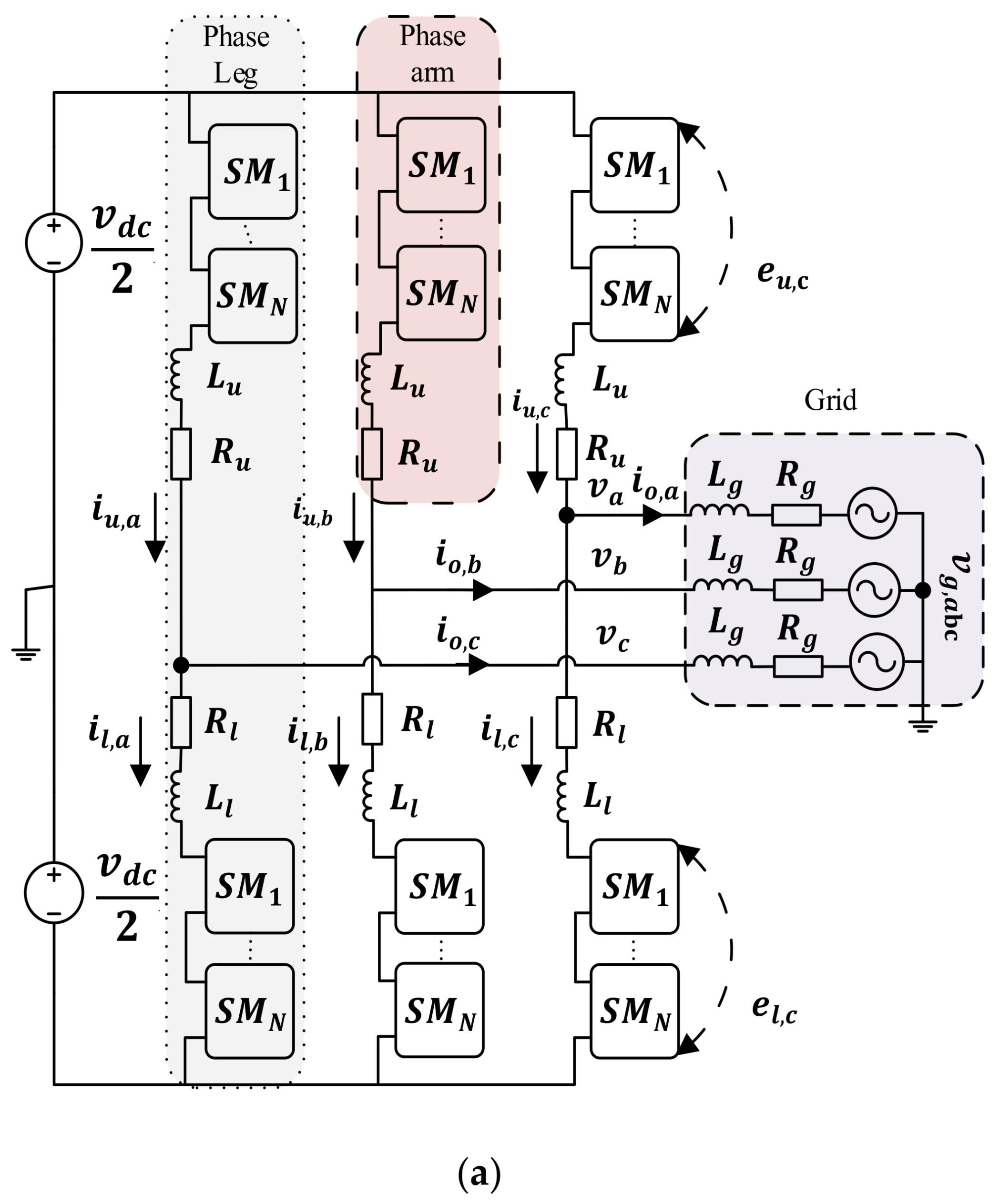
The configuration of MMC is composed of upper arms and lower arms, as depicted in Figure 1a. The upper and lower arm combinedly form a phase leg. Moreover, the arm of MMC is composed of $N$ submodules, which are connected in series with arm inductor $L_{u,l}$, and the series equivalent resistor $R_{u,l}$. The SM has a half-bridge configuration, consists of two switches $(S_1$, $S_2),$ and storage capacitor $C$, as depicted in Figure 1b. The values of the different parameters of MMC are given in

Table 1. MMC parameters.

Parameters	Symbol	Value
Sampling time	Ts	1 × 10−5 s
Rated power of MMC	$P_{rated}$	50 kW
No of submodules in arm	$N$	4
DC link voltage	$V_{dc}$	622 V
Grid phase voltage (peak)	$v_j$	311 V
Submodule capacitance	$C$	0.0048 F
Arm inductor	$L$	1.8 mH
Arm resistor	$R$	0.056 Ω
Grid inductor	$L_g$	99.035 μ
Grid resistor	$R_g$	0.0031 Ω

. These SMs are either inserted or bypassed with the operation of switches $(S_1$, $S_2)$. The output of these submodules combinedly gives the output voltage of MMC. With $S_1$ turned on and $S_2$ turned off, the SM capacitor will insert in the current path, and the SM capacitor is bypassed by turning on $S_2$ and turning off $S_1$. However, turning off both switches will result in the blocking of SM. This condition is used during fault to divert current to an antiparallel diode, which has a higher current carrying capability than transistors. By appropriately applying switching signal to these switches, the arm voltage can be varied between zero and the sum of all SM voltages, i.e., $0\le e_{u,l}\le v_{cu,l}^{\Sigma }$

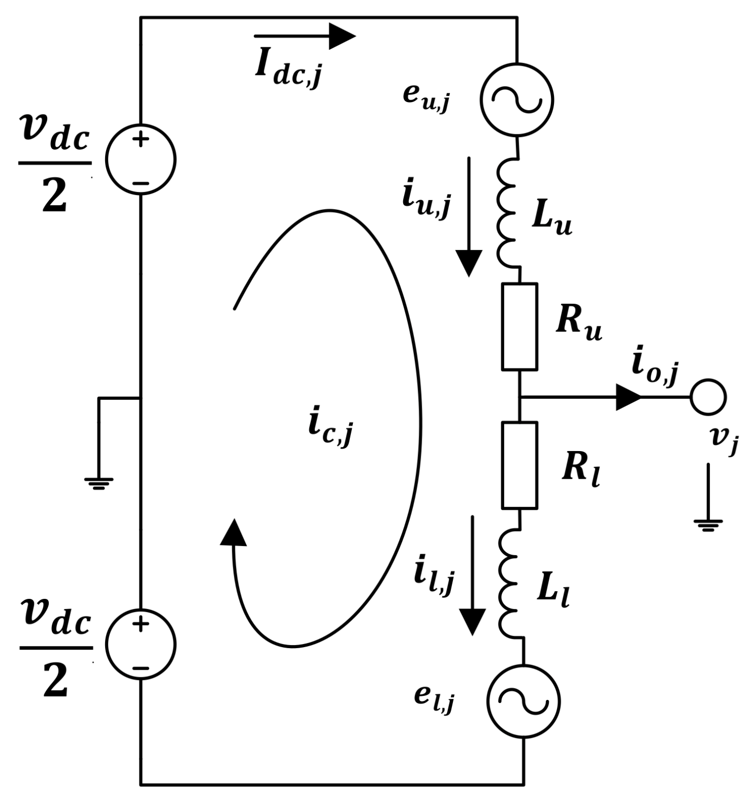
The mathematical model of MMC is derived from the phase equivalent circuit given in Figure 2. When Kirchhoff’s voltage law is applied to the upper and lower loop, it will result in (1a) and (1b) [28,29].

$$\frac{1}{2}{v}_{dc}-e_{u,j}-i_{u,j}{R}_u-L_u\frac{d{i}_{u,j}}{dt}=v_j$$

(1a)

$$-\frac{1}{2}{v}_{dc}+e_{l,j}+i_{l,j}{R}_l+L_l\frac{d{i}_{l,j}}{dt}=v_j$$

(1b)

As the SMs are composed of capacitors and a combination of switches $(S_1$, $S_2)$, its dynamics are modeled as

$$\frac{C}{N}\frac{d{v}_{cu,j}^{\Sigma }}{dt}=n_{u,j}^i{i}_{u,j}$$

(2a)

$$\frac{C}{N}\frac{d{v}_{cl,j}^{\Sigma }}{dt}=n_{l,j}^i{i}_{l,j}$$

(2b)

Moreover, the relationship between different currents is derived by applying Kirchhoff’s current law. The resulting currents are given as follows:

$$i_{u,j}=i_{c,j}+\frac{i_{o,j}}{2}$$

(3a)

$$i_{l,j}=i_{c,j}-\frac{i_{o,j}}{2}$$

(3b)

The summation and subtraction of (3a) and (3b) give the output current and circulating current.

$$i_{o,j}=i_{u,j}-i_{l,j}$$

(4a)

$$i_{c,j}=\frac{1}{2}\left(i_{u,j}+i_{l,j}\right)$$

(4b)

The circulating current is composed of a DC component and different harmonic components. It can be represented by a general expression as

$$i_{c,j}=\frac{I_{dc,j}}{3}+i_{ch,j}$$

(5)

$i_{ch,j}$ is an undesirable component that is composed of different harmonic components given as follows:

$$i_{ch,j}={\displaystyle \sum }_{h=1}^{\infty }{I}_h\cos (h\omega t)$$

(6)

3. Control Design

The differential voltage equations of the upper arm (1a) and lower arm (1b) are transformed into the Laplace domain, as given below. These equations indicate the dynamic response of MMC arm currents.

$$i_{u,j}=\frac{1}{L_u.s+R_u}\left(\frac{1}{2}{v}_{dc}-v_j-e_{u,j}\right)$$

(7a)

$$i_{l,j}=\frac{1}{L_l.s+R_l}\left(\frac{1}{2}{v}_{dc}+v_j-e_{l,j}\right)$$

(7b)

Equations (7a) and (7b) show that $e_{u,j}$ and $e_{l,j}$ are the only available variable for control of the upper-arm and lower-arm currents. The upper-arm and lower-arm voltages are manipulated to achieve the desired response of circulating current and output current with a regulated SM capacitor voltage.

The control objectives in this paper are to control output current to ensure the delivery of desired active and reactive power to the grid and regulating circulating current such that it tracks DC current reference and eliminates its second harmonic components. These objectives are achieved by implementing a control algorithm in SRF $\left(\alpha \beta \gamma \right)$. The three-phase arm current ($i_{u,l}^{abc}$) is transformed into $i_{u,l}^{\alpha \beta \gamma }$. Unlike the balance system, here, the gamma $\gamma$ component is not zero. It represents the DC current flowing in each arm on MMC. By Clark transformation [30], upper arm and lower arm currents $\left(i_{u,l}^{abc}\right)$ will decompose to their respective $\alpha \beta \gamma$ components $\left(i_{u,l}^{\alpha \beta \gamma }\right)$, as given below.

$$i_{u,l}^{\alpha \beta \gamma }=\left[T_{\alpha \beta \gamma }\right]i_{u,l}^{abc}$$

(8a)

$$\left[T_{\alpha \beta \gamma }\right]=\frac{2}{3}\left[\begin{array}{ccc}1& -\frac{1}{2}& -\frac{1}{2}\\ 0& \frac{\sqrt{3}}{2}& -\frac{\sqrt{3}}{2}\\ \frac{1}{2}& \frac{1}{2}& \frac{1}{2}\end{array}\right]$$

(8b)

$$\left[\begin{array}{c}{i}_{\alpha u,l}\\ i_{\beta u,l}\\ i_{\gamma u,l}\end{array}\right]=\left[\begin{array}{c}\frac{1}{3}\left(\begin{array}{c}\left(i_{ul,a}-\frac{1}{2}{i}_{ul,b}-\frac{1}{2}{i}_{ul,c}\right)+\\ \left(2i_{2ul,a}-i_{2ul,b}-i_{2ul,c}\right)\end{array}\right)\\ \frac{1}{\sqrt{3}}\left(\left(\frac{1}{2}{i}_{ul,b}-\frac{1}{2}{i}_{ul,c}\right)+\left(i_{2ul,b}-i_{2ul,c}\right)\right)\\ \frac{I_{dc}}{3}\end{array}\right]$$

(8c)

The values of arm currents in (8c) are substituted with (3a) and (3b). By supposing positive sequence and output current $i_{oa}=I\cos \omega t$ and second harmonic current $i_{2a}=I_2\cos (2\omega t)$, (8c) is calculated for upper-arm currents as

$$\left[\begin{array}{c}{i}_{\alpha u}\\ i_{\beta u}\\ i_{\gamma u}\end{array}\right]=\left[\begin{array}{c}\frac{1}{2}I\cos \omega t+I_2\cos (2\omega t)\\ \frac{1}{2}I\sin \omega t-I_2\sin (2\omega t)\\ \frac{I_{dc}}{3}\end{array}\right]$$

(9a)

Similarly, the lower-arm current is represented in SRF as

$$\left[\begin{array}{c}{i}_{\alpha l}\\ i_{\beta l}\\ i_{\gamma l}\end{array}\right]=\left[\begin{array}{c}-\frac{1}{2}I\cos \omega t+I_2\cos (2\omega t)\\ -\frac{1}{2}I\sin \omega t-I_2\sin (2\omega t)\\ \frac{I_{dc}}{3}\end{array}\right]$$

(9b)

Generally, the arm current can be represented as

$$i_{u,l}=f\left(i_{\alpha u,l}, i_{\beta u,l}, i_{\gamma u,l}\right)$$

(10)

Equation (10) shows that the arm current is a function of all three ($\alpha \beta \gamma$) components of SRF.

The circulating current can be represented in SRF as

$$i_{c,\alpha \beta \gamma }=\frac{1}{2}\left(\underset{i_{u,abc}}{\underbrace{\left(i_{\alpha u}+i_{\beta u}+i_{\gamma u}\right)}}+\underset{i_{l,abc}}{\underbrace{\left(i_{\alpha l}+i_{\beta l}+i_{\gamma l}\right)}}\right)$$

(11)

Equation (11) shows that if the $\alpha \beta \gamma$ components of the upper-arm and lower-arm currents are kept 180° apart, i.e., $i_{\alpha \beta ,u}=-i_{\alpha \beta ,l}$, we can eliminate the AC component of the circulating current, which will result in only a DC component.

Let us assume $i_{\alpha \beta ,u}=-i_{\alpha \beta ,l}$.

$$\left\{\begin{array}{l}{i}_{u\alpha }=\frac{1}{2}I\cos \omega t+I_2\cos (2\omega t) \mathrm{Then}\\ i_{l\alpha }=\frac{1}{2}I\cos (\omega t+{180}^{°})+I_2\cos (2\omega t+{180}^{°})\end{array}\right.$$

(12a)

$$\left\{\begin{array}{l}{i}_{u\beta }=\frac{1}{2}I\sin \omega t-I_2\sin (2\omega t) \mathrm{Then}\\ i_{l\beta }=\frac{1}{2}I\sin (\omega t+{180}^{°})-I_2\sin (2\omega t+{180}^{°})\end{array}\right.$$

(12b)

For finding mathematical relation of the circulating current in SRF substitute (12a), (12b) in (11), and adding the same components, we obtain

$$\left(i_{u,\alpha }+i_{l,\alpha }\right)=\left(\frac{1}{2}I\cos \omega t+I_2\cos (2\omega t)+I\cos (\omega t+180°)+I_2\cos (2\omega t+180°)\right)$$

(13a)

$$\left(i_{u,\beta }+i_{l,\beta }\right)=\left(\frac{1}{2}I\sin \omega t-I_2\sin (2\omega t)+I\sin (\omega t+180°)-I_2\sin (2\omega t+180°)\right)$$

(13b)

$$\left(i_{u,\gamma }+i_{l,\gamma }\right)=\left(\frac{I_{dc}}{3}+\frac{I_{dc}}{3}\right)$$

(13c)

The right sides of (13a) and (13b) are expanded by using basic trigonometric identity given as

$$\cos \left(\alpha \pm \beta \right)=\cos \alpha \cos \beta \mp \sin \alpha \sin \beta$$

(14a)

$$\sin \left(\alpha \pm \beta \right)=\sin \alpha \cos \beta \pm \cos \alpha \sin \beta$$

(14b)

The result obtained from (13) is substituted in (11); hence, the different components of circulating current in SRF are represented as

$$\left[\begin{array}{c}{i}_{c,\alpha }\\ i_{c,\beta }\\ i_{c,\gamma }\end{array}\right]=\left[\begin{array}{c}0\\ 0\\ \frac{I_{dc}}{3}\end{array}\right]$$

(15)

The circulating current will remain only with the DC component given as

$$i_{c,\alpha \beta \gamma }=\frac{I_{dc}}{3}$$

(16)

Equation (16) confirms that by choosing a proper reference for the upper arm and lower arm, and the $\alpha \beta$ component of circulating current can be eliminated. The only component that remained behind is $\gamma$ component, which is the desired DC component of circulating current.

Similarly, the output current is calculated by putting the supposed value of the upper arm and lower arm current from (12a) and (12b) to (4a), which gives

$$i_{o,\alpha }=\left(\frac{1}{2}I\cos \omega t+I_2\cos (2\omega t)-\frac{1}{2}I\cos (\omega t+180°)-I_2\cos (2\omega t+180°)\right)$$

(17a)

$$i_{o,\beta }=\left(\frac{1}{2}I\sin \omega t-I_2\sin (2\omega t)-\frac{1}{2}I\sin (\omega t+180°)+I_2\sin (2\omega t+180°)\right)$$

(17b)

$$i_{o,\gamma }=\frac{I_{dc}}{3}-\frac{I_{dc}}{3}$$

(17c)

Equations (14a) and (14b) are used to simplify (17a) and (17b). The result is given as

$$\left[\begin{array}{c}{i}_{o,\alpha }\\ i_{o,\beta }\\ i_{o,\gamma }\end{array}\right]=\left[\begin{array}{c}I\cos \omega t\\ I\sin \omega t\\ 0\end{array}\right]$$

(18)

Equation (18) shows that the output current is only composed of a fundamental frequency component. The output current is equal to two times of upper arm current, i.e., $i_{o,\alpha \beta }=2i_{\alpha \beta ,u}$. The output current is represented as

$$i_o=I\cos \omega t+jI\sin \omega t$$

(19)

From (16) and (19), we have concluded that by choosing proper references for the upper arm and lower arm current, the circulating current can be forced to track DC reference by eliminating double frequency AC component, while output current can be set to deliver require power to a connected grid. It will not affect the output current.

3.1. Reference Generation

The important step in this control algorithm is to generate a proper reference for arm currents so that it will deliver desired active and reactive power to the grid along with the regulation of circulating current to its DC reference value. The references for $i_{ul,\alpha \beta }$ and $i_{ul,\mathsf{\gamma }}$ are generated from reference power delivered by the converter. From p–q theory in [30], the power in SRF is given as

$$\left[\begin{array}{c}{p}_{\gamma }\\ p\\ q\end{array}\right]=\left[\begin{array}{ccc}{v}_{\gamma }& 0& 0\\ 0& v_{\alpha }& v_{\beta }\\ 0& v_{\beta }& -v_{\alpha }\end{array}\right]\left[\begin{array}{c}{i}_{\gamma }\\ i_{\alpha }\\ i_{\beta }\end{array}\right]$$

(20)

The references for upper arm currents are achieved by taking the inverse of the matrix as

$$\left[\begin{array}{c}{i}_{u\gamma }^{\ast }\\ i_{u\alpha }^{\ast }\\ i_{u\beta }^{\ast }\end{array}\right]=\frac{1}{3}\left[\begin{array}{ccc}\frac{1}{v_{\gamma }}& 0& 0\\ 0& \frac{v_{\alpha }}{v_{\alpha }^2+v_{\beta }^2}& \frac{v_{\beta }}{v_{\alpha }^2+v_{\beta }^2}\\ 0& \frac{v_{\beta }}{v_{\alpha }^2+v_{\beta }^2}& \frac{-v_{\alpha }}{v_{\alpha }^2+v_{\beta }^2}\end{array}\right]\left[\begin{array}{c}{p}_r^{\ast }\\ p^{\ast }\\ q^{\ast }\end{array}\right]$$

(21)

$i_{\gamma }^{\ast }$ is DC current component, which is circulating in each arm. It is equal to $\frac{I_{dc}}{3},$ while $v_{\gamma }$ is DC link voltage, which is equal to $v_{dc}$. $p_r^{\ast }$ is equal to $p^{\ast }+p_{loss}$. If the losses are ignored, then these terms can be used interchangeably. The reference of the upper arm current is generated from (21). While the reference of lower arm current is set such that it has a 180° phase shift with the reference of upper arm current.

$$i_{l,\alpha \beta }^{\ast }=-i_{u,\alpha \beta }^{\ast }$$

(22)

The term $i_{ul,\alpha \beta }^{\ast }$ will combinedly control the output active and reactive power of MMC. However, the $i_{ul,\gamma }^{\ast }$ is responsible for power transfer from the DC port to the AC port. In reference generation, $p^{\ast }$ and $q^{\ast }$ can be any real values, but the terminal voltage $v_j$ is sensed and passed through a Second Order Generalized Integrator-Phase Locked Loop (SOGI-PLL), as the output voltage of MMC is composed of different harmonics components. In order to achieve a good reference for better control performance, the positive sequence of the output voltage is extracted using the SOGI quadrature signal generator (QSG) [31]. The structure of SOGI is depicted in Figure 3.

$$\frac{v^{\prime }\left(s\right)}{v\left(s\right)}=\frac{k\omega s}{s^2+k\omega s+{\omega }^2}$$

(23a)

$$\frac{q{v}^{\prime }\left(s\right)}{v\left(s\right)}=\frac{\omega }{s}\frac{v^{\prime }\left(s\right)}{v\left(s\right)}=\frac{k{\omega }^2}{s^2+k\omega s+{\omega }^2}$$

(23b)

where $q$ is 90° lagging phase shift operator, i.e., $q=e^{-j\frac{\pi }{2}}$. The value of $k$ is set to $\raisebox{1ex}{$\sqrt{2}$}\!\left/ \!\raisebox{-1ex}{$2$}\right.$. The SOGI-QSG generates the direct and in-quadrature components for the input vector. These signals are used to calculate the positive sequence of the respective input signal.

$$G_f\left(s\right)=\left[\begin{array}{c}{v}_{\alpha }^{+}\\ v_{\beta }^{+}\end{array}\right]=\frac{1}{2}\left[\begin{array}{cc}1& -q\\ q& 1\end{array}\right]\left[\begin{array}{c}{v}_{\alpha }^{\prime }\\ v_{\beta }^{\prime }\end{array}\right]$$

(24)

Equation (21) is used to calculate pure sinusoidal reference current for the upper arm, and Equation (22) is used to generate a reference for the lower arm.

Keeping in view the nature of currents as given in (9a) and (9b), a PR controller is used for controlling $\alpha \beta$-component, while $\gamma$-component is controlled using a proportional controller. Hence, the control law is designed as

$$\left\{\begin{array}{c}{e}_{u,j}^{\ast }=\frac{v_{dc}}{2}-R{i}_{u,\alpha \beta \gamma }^{\ast }-(k_p+{\displaystyle {\displaystyle \sum }_{h=1}^2}\left(\frac{2k_{rh}s}{s^2+{\left(h\omega \right)}^2}\right)e_1-v_j\\ e_{u,j}^{\ast }=\frac{v_{dc}}{2}-R{i}_{l,\alpha \beta \gamma }^{\ast }-(k_p+{\displaystyle {\displaystyle \sum }_{h=1}^2}\left(\frac{2k_{rh}s}{s^2+{\left(h\omega \right)}^2}\right)e_2+v_j\end{array}\right.$$

(25a)

$$\left\{\begin{array}{c}{e}_1=i_{u,\alpha \beta \gamma }^{\ast }-i_{u,\alpha \beta \gamma }\\ e_2=i_{l,\alpha \beta \gamma }^{\ast }-i_{l,\alpha \beta \gamma }\end{array}\right.$$

(25b)

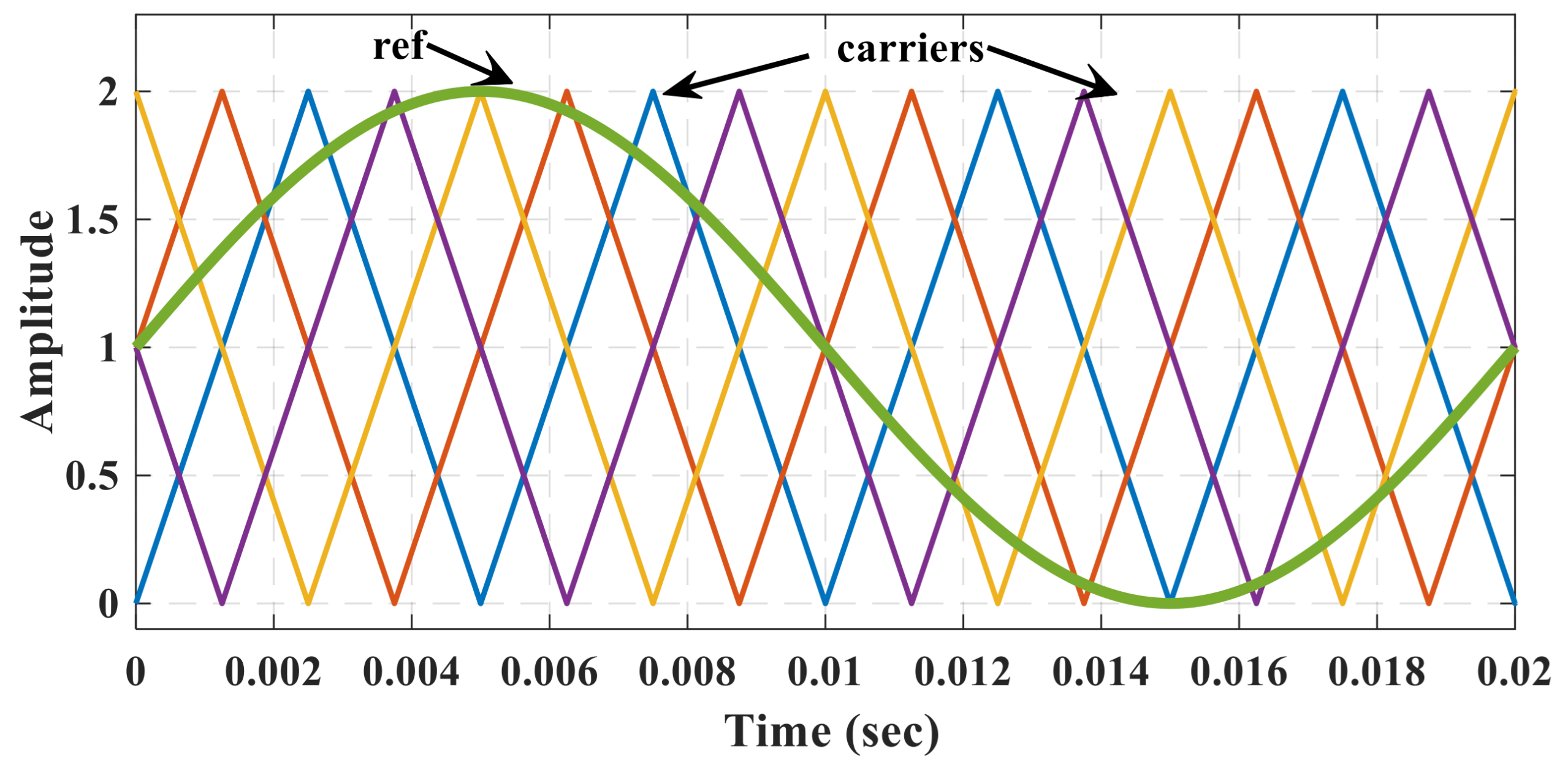
Equations (25a) and (25b) represent the control input to the plant. The insertion indices signal for both arms is achieved by dividing the control signal by $\frac{V_d}{2}$ and is fed to PS-PWM to generate a gating signal for MMC. The reference output voltage is given as

$$v_j^{\ast }=m\frac{v_{dc}}{2}\sin \omega t$$

(26)

Finally, the reference signals for the upper arm and lower arm are as follows:

$$e_{u,a}^{\ast }=\frac{v_{dc}}{2}\left(1-m\sin \omega t\right)$$

(27a)

$$e_{l,a}^{\ast }=\frac{v_{dc}}{2}\left(1+m\sin \omega t\right)$$

(27b)

The modulation and carrier signal is depicted in Figure 4.

3.2. Proportional Resonant Controller

PR controller is a good choice for reference tracking in a stationary frame. PI controller provides infinite gain at DC frequency, which eliminates the steady-state error. Similarly, the PR controller provides infinite gain at a specific frequency ($\omega$) for eliminating steady-state error [32]. The transfer function of the PR controller is given as

$$C_{PR}\left(s\right)=k_p+{\displaystyle {\displaystyle \sum }_{h=1}^n}\left(\frac{2k_{rh}s}{s^2+{\left(h\omega \right)}^2}\right)$$

(28)

where $k_p$ is the proportional gain, while $k_{rh}$ is a resonant gain for $h$ resonant term. The $k_p$ play a critical role in controller design as it decides the bandwidth, gain and phase margin of the system. The $k_{rh}$ shifts the response magnitude vertically without affecting the bandwidth of the controller.

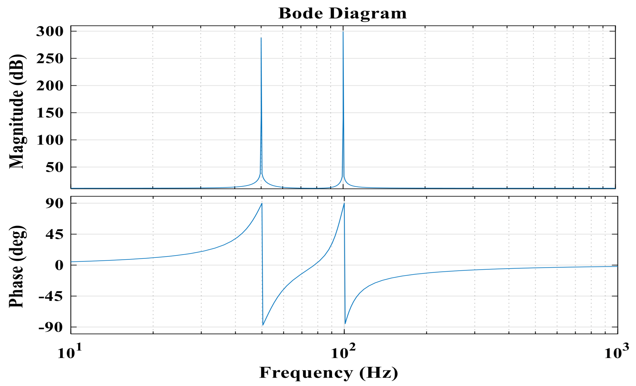
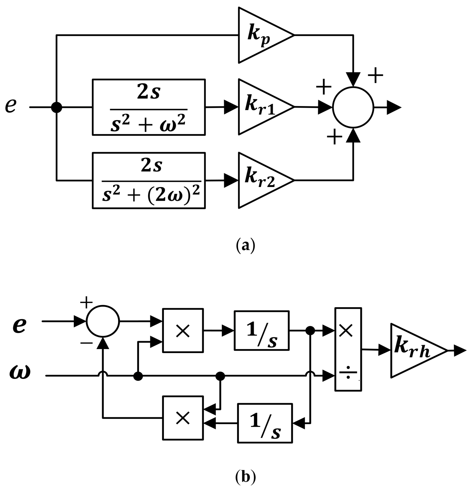
As shown in (9a) and (9b), the arm current is composed of a fundamental frequency component as well as its second harmonic component, the controller is tuned at these two frequencies to achieve a desired control input signal. The transfer function for the controller is achieved by expanding (28) for $n=2$, since we are dealing with the fundamental frequency and its second component. The bode diagram for resulted PR controller is given in Figure 5, which shows high gain at fundamental as well as double frequency. The structure of the controller is depicted in Figure 6a, and its mathematical form is given as

$$C_{PR}\left(s\right)=k_p+\frac{2k_{r1}s}{s^2+{\left(\omega \right)}^2}+\frac{2k_{r2}s}{s^2+{\left(2\omega \right)}^2}$$

(29)

Equation (29) shows the mathematical expression of the PR controller, which is implemented for controlling the output and circulating current of MMC.

The resonant part of the controller is implemented with second-order generalize integrator (SOGI), as depicted in Figure 6b.

3.3. Parameter Tuning of PR

The selection of the proper parameter of the PR controller is very crucial in stable closed-loop operation. The parameter defines the bandwidth, which determines the exponential rate of convergence of the system [28]. Hence, the value of $k_p$ is calculated by considering the bandwidth of output control. It is calculated as

$$k_p=L_{u,l}{b}_w$$

(30)

where $b_w$ is the desired bandwidth of the closed-loop system. A useful rule of thumb for selecting the bandwidth for the stability of the system is given as [28]

$$b_w\le \frac{{\omega }_s}{10}\hspace{1em}\hspace{1em}{\omega }_s=\frac{2\pi }{T_s}$$

(31)

where ${\omega }_s$ and $T_s$ are angular sampling frequency and sampling time, respectively. Moreover, the resonant gain $k_{rh}$ is selected as

$$k_{rh}=2b_h{k}_p$$

(32)

where $b_h$ is resonant bandwidth. It determines the exponential rate of convergence of the resonant part, which plays a role in accurately tracking reference values. Its value must be selected as

$$b_h\ll b_w$$

(33)

More specifically, resonant bandwidth should be less than the angular frequency of the grid, as given below.

$$b_h<\omega$$

(34)

The values of PR parameters are selected based on these calculations. The value of proportional and resonant gains, bandwidth, and sampling time are given in

Table 2. Controller tuning parameters.

Parameters	Value
$k_p$	3.5653
$b_w$	2000
$b_1$	50
$k_{r1}$	356.5253
$b_2$	200
$k_{r2}$	400
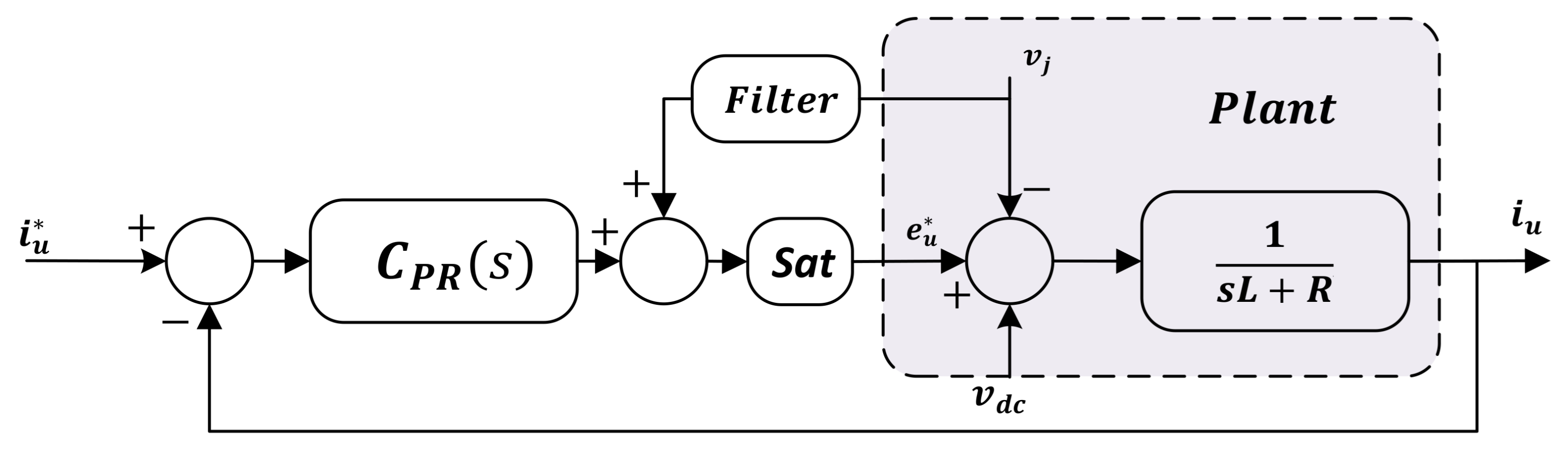
$T_s$	1 × 10−5 s

. The generalized control structure is given in Figure 7, while the complete control scheme based on the arm-based control and comparative leg-level control is depicted in Figure 8.

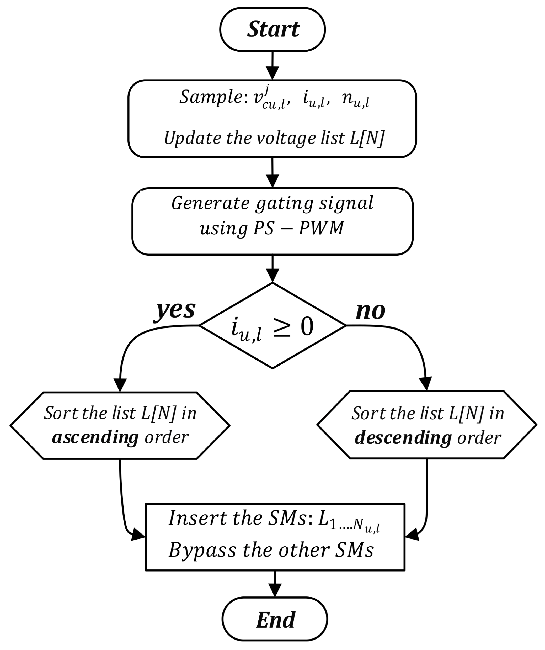
The regulation of capacitor voltage is important for the proper operation of MMC. A conventional capacitor sorting algorithm is used for the regulation of capacitor voltages. The choice of switching of SM is made in such a way that SM with extreme voltages ($v_{sm}$) are chosen to prevent its deviation from the mean value. A conventional sorting algorithm in [33] is used in conjunction with nearest level control. However, in our paper, it is used in combination with PS-PWM. The algorithm requires three variables, i.e., capacitor voltage, arm currents, and insertion indices for generating desired PWM signal to regulate the capacitor voltages. The flow chart of the algorithm is depicted in Figure 9.

The main cases of this conventional algorithm are given as follows:

• If the arm current is greater than zero, then the bypassed SM with the lowest $v_{sm}$ is selected for insertion since it will charge the capacitor and SM with the highest $v_{sm}$ is bypassed because further charging will deviate the capacitor voltage from its mean value.
• In the case of a negative current, the SM with the highest $v_{sm}$ is chosen for insertion because this will result in discharging of the capacitor, and the SM with the lowest $v_{sm}$ is bypassed since its insertion will completely discharge the capacitor resulting in almost zero SM capacitor voltage.

4. Results and Discussion

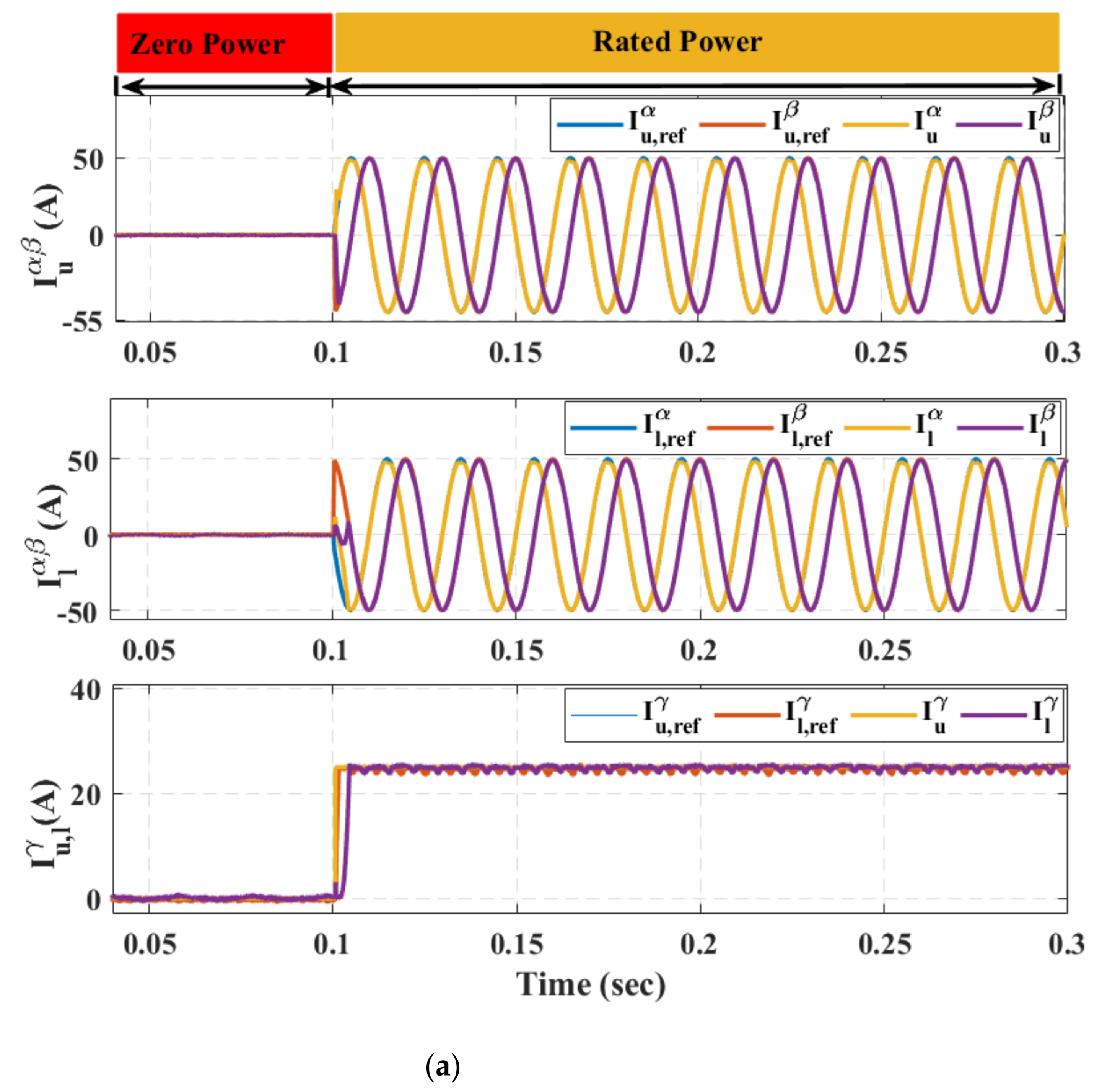
A three-phase, five-level MMC is designed in MATLAB/Simulink to verify the proposed control scheme. To verify the effectiveness of the control scheme, the reference of output current is kept at zero till 0.1 s (zero power mode), which means that the converter is not injecting active power to the grid. At t = 0.1 s, rated power is injected into the grid (rated power mode). That will change the reference output current from zero to 100 A. This large variation is created to ensure the effectiveness of the control method. Moreover, the comparative results of output current, circulating current, and SM capacitor voltage obtained from leg-level control are presented for comparison. The control scheme implemented for leg-level control and arm-level control is depicted in Figure 8. The results of different parameters subjected to step change in active power are given in Figure 10, Figure 11, Figure 12, Figure 13, Figure 14, Figure 15 and Figure 16. 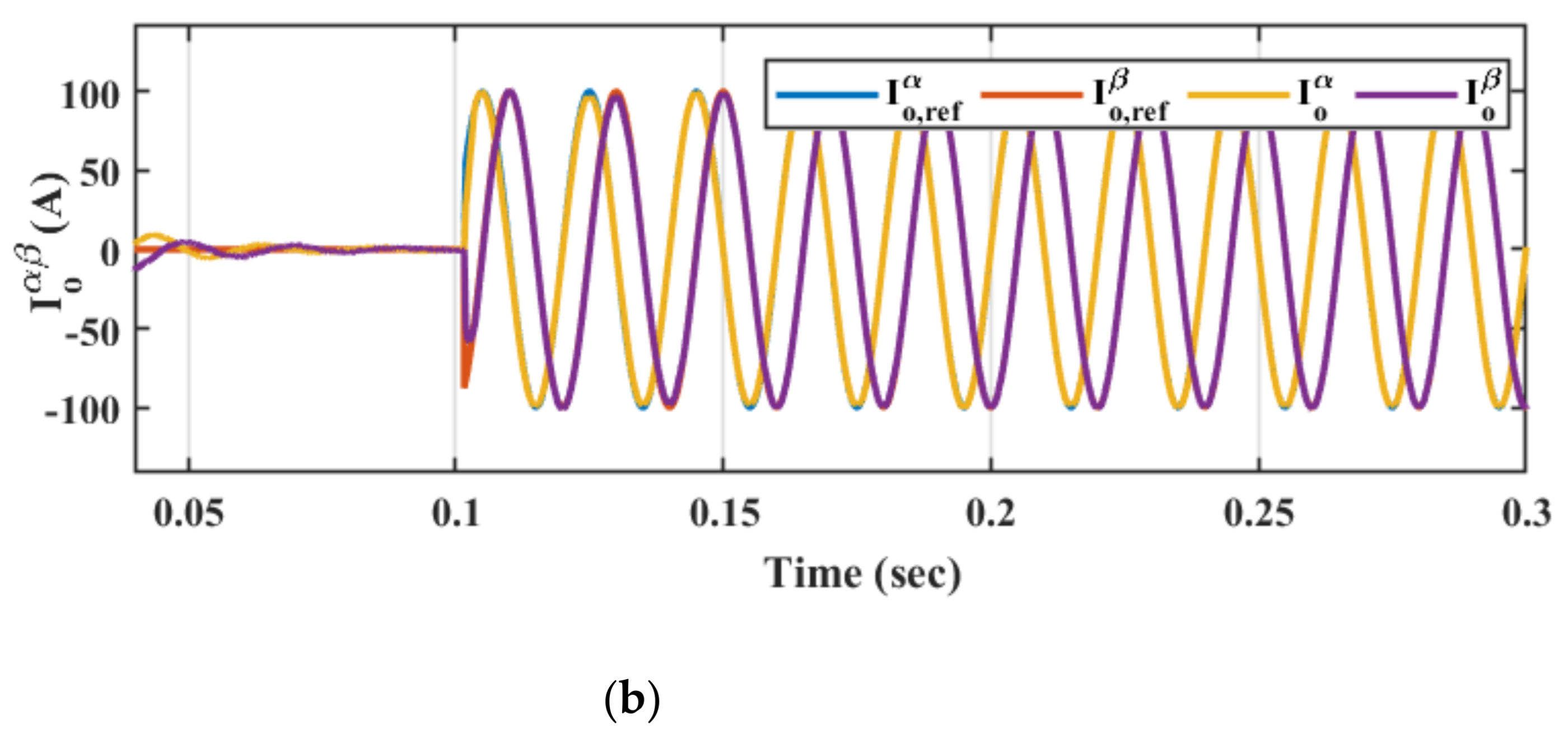Figure 10a depicts the upper-arm and lower-arm currents in SRF. The three components of the current $i_{u,l}^{\alpha \beta \gamma }$ are controlled effectively. The measure values of the arm current are tracking its desired value perfectly. With the step change in power, the reference of arm current components $i_{u,l}^{\alpha \beta }$ increases from 0 A to around 50 A peak. Similarly, the DC component $i_{u,l}^{\gamma }$ also changes from 0 A to 25 A. The controller is keeping the measured value at zero since the reference is set to zero. As the power changes from zero to rated power, the arm current also starts tracking its reference value. With the change of reference, the controller output changes quickly and continues its tracking. Figure 10b shows the control response of the leg-level control scheme. Similar to the arm level, the tracking of the controller in SRF is good. The reference value is well tracked.

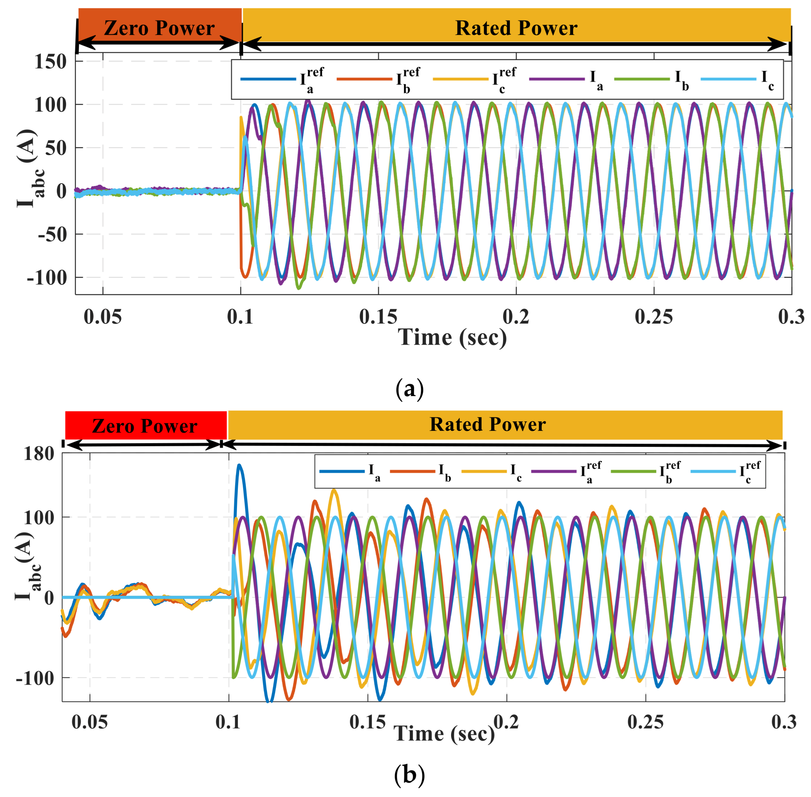
Figure 11 shows the reference and measured output current obtained from arm-level control as well as from leg-level control. In Figure 11a, the upper- and lower-arm currents are combined to obtain the output current. The effective tracking of arm currents has enabled the output current to follow its reference without any error. This will assure the transfer of the required power to the grid. The quality of output current is checked by carrying out its fast Fourier transform (FFT) analysis, depicted in Figure 12. The FFT analysis shows that the THD is 2.98%, which fulfills the IEEE standard for THD. However, in Figure 11b, the response of leg-level control is presented. Although the current was effectively controlled in SRF, here, it is clearly depicted that the current response is not appreciable. The controlled current is settled after 0.25 s, and still, the steady-state error is visible by closely analyzing the figure.

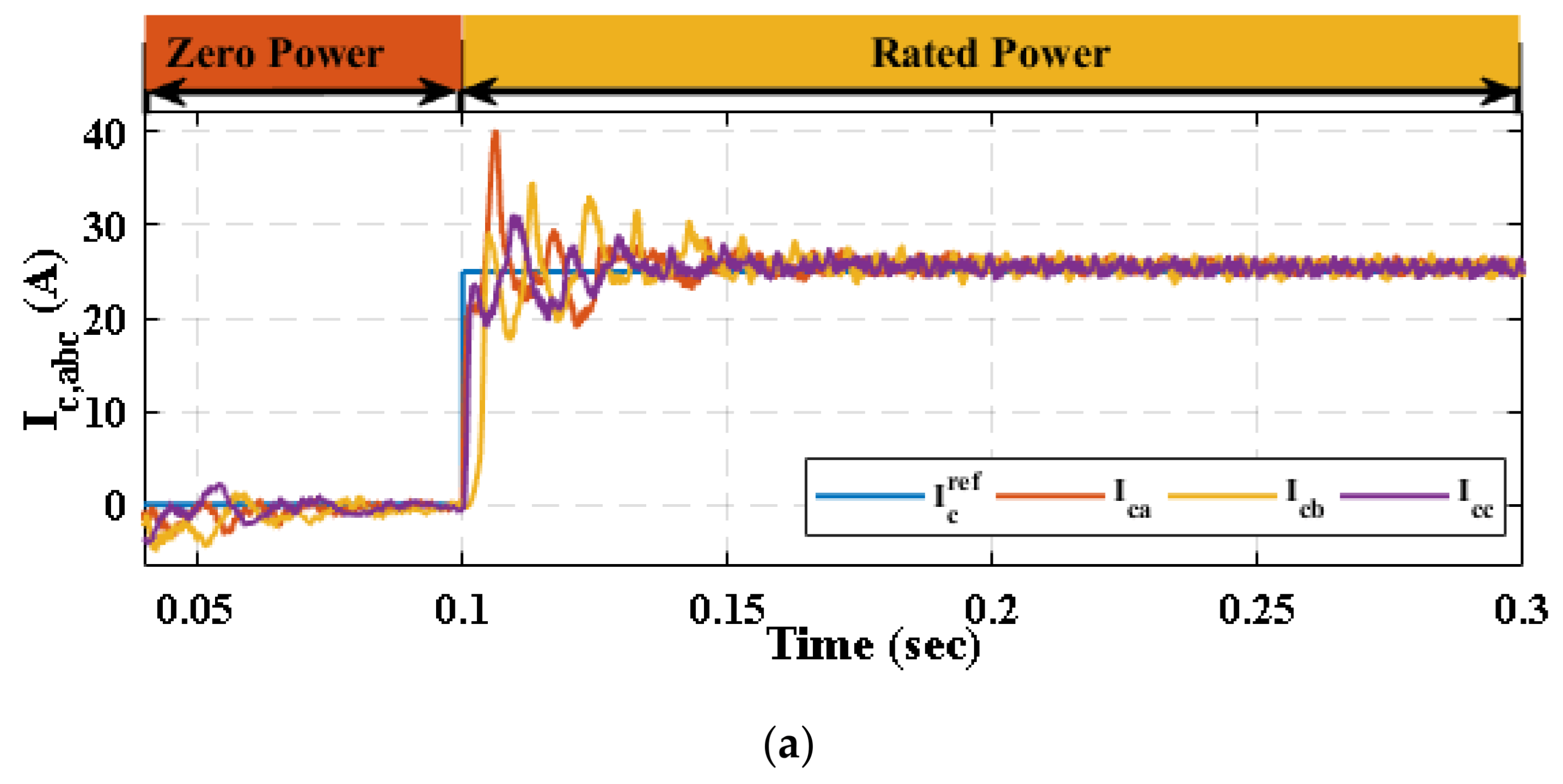
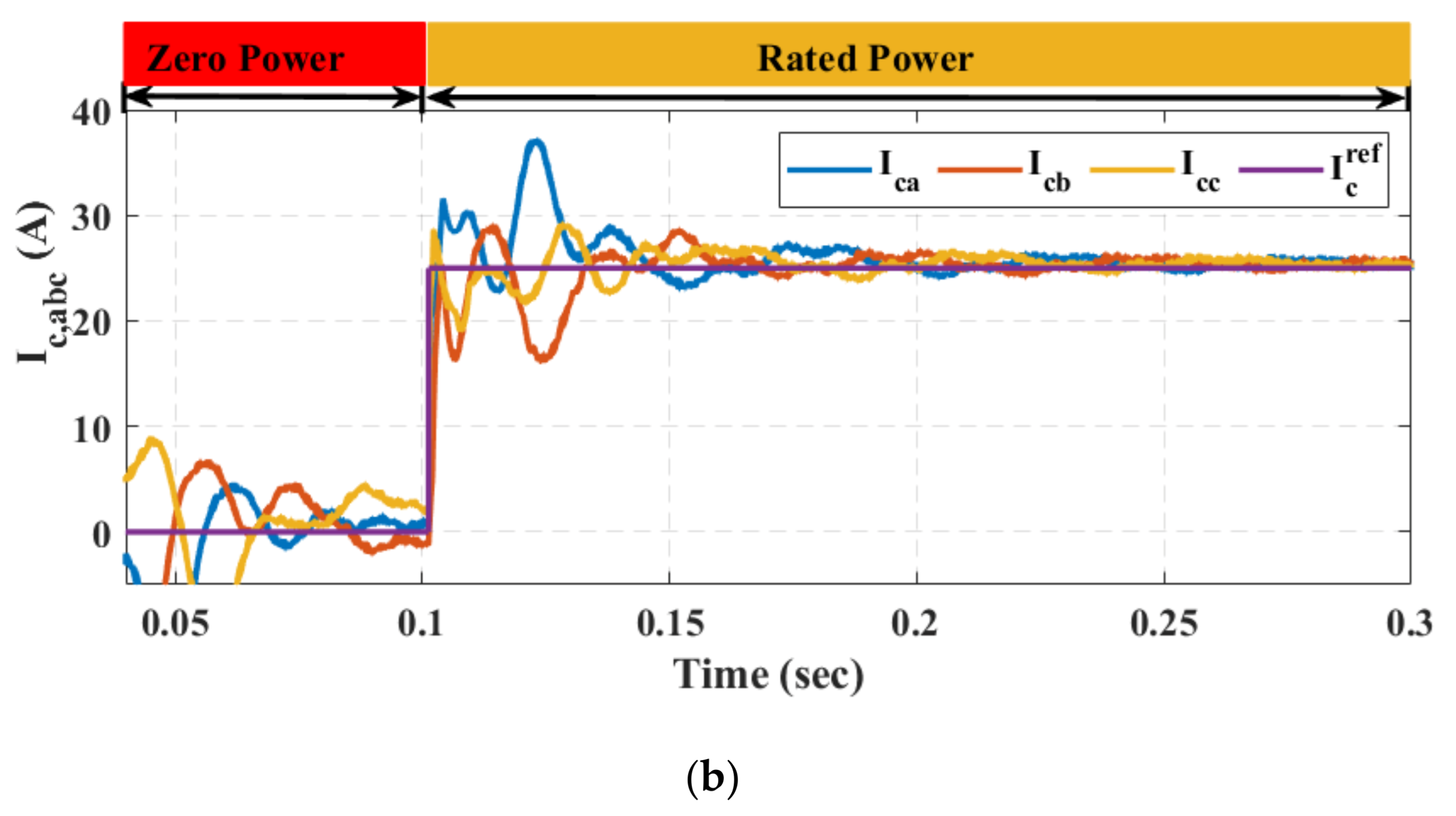
The circulating current of all three-phase of MMC for both arm-level and leg-level control is depicted in Figure 13. The uncontrolled circulating current has both double frequency AC and DC components. The DC component is used to transfer power from the DC port to the AC port, while the AC component of the circulating current is completely undesirable, which has a negative impact on the converter. As shown in Figure 13a, the differential current only contains the DC component, while its AC term is eliminated. This validates the proposed control scheme. At zero injection mode, the current is zero, following its reference value, but when the mode is changed to rated power, the current is changed from zero to 25 A. As the power mode changed, the current shows some overshoot due to the sudden change in power reference. The control scheme has the ability to tackle the changes to settle the measured current on its reference value, resulting in the complete elimination of the second harmonic component. However, Figure 13b shows the circulating current obtained from the leg-level control. The current response is slow and settled around 0.25 s, while in the case of arm level, it is settled around 0.15 s. After switching the converter to rated power mode, the circulating current shows large variation in the case of leg-level control.

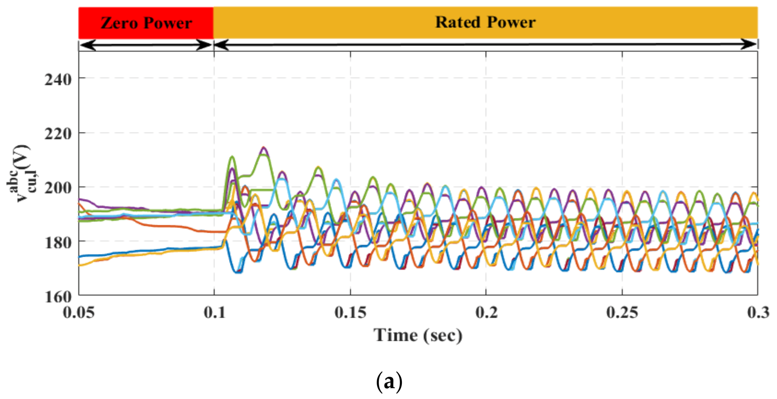
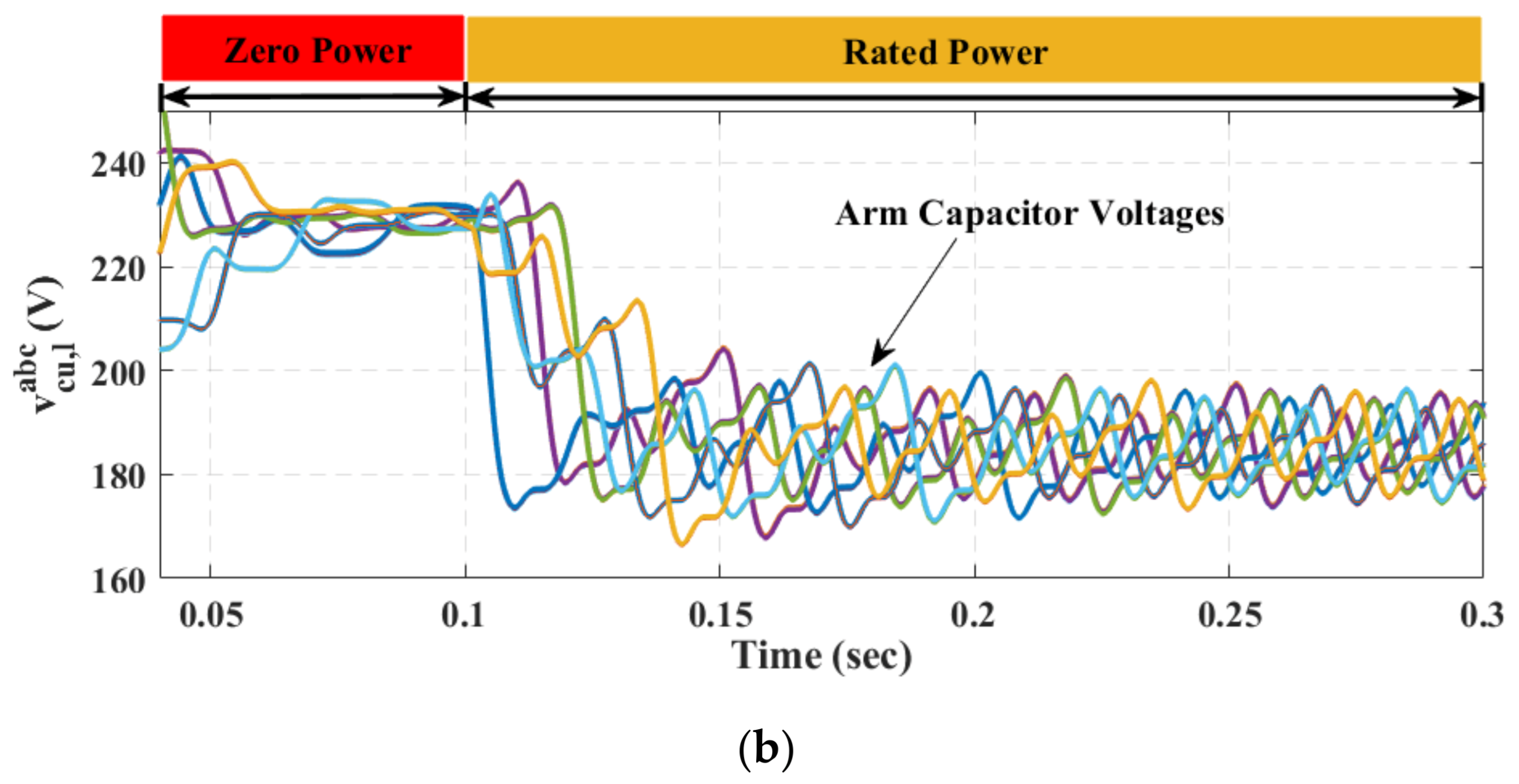
The arm capacitor voltage of all three phases is shown in Figure 14. Its mean value is regulated to 155 V ($\frac{V_{dc}}{N}$). As no power is injected into the grid at the start, the capacitors are fully charged and holding the energy. At this instant, the capacitor voltage has no ripple, and it is almost constant. Since the power mode is changed from zero to rated power, and the converter starts injecting power to the grid, the capacitor voltage is subjected to the fluctuation, which is known as ripples. Even the current reference is changed at t = 0.1 s; still, the sorting algorithm is effective by keeping constant the means values. In the case of arm-level, the mean value is constant during both zero and rated power mode, while in the case of leg-level control, at zero power, the mean value of capacitor voltage deviates more from its reference value. Additionally, in the rated-power case, the value of capacitor voltage is higher than the desired value. The better comparison and quick analysis of the performance indices are measured for both control strategies and presented in

Table 3. Performance indices of controllers.

Parameters	Performance Indices	Arm Level			Leg Level
		Phase a	Phase b	Phase c	Phase a	Phase b	Phase c
$i_o$	ITAE	0.04636	0.0449	0.0566	0.2089	0.2906	0.2768
	IAE	1.574	1.716	1.429	4.875	5.576	4.495
	ISE	185.7	257.8	192.9	474.5	720.4	385.5
$i_c$	ITAE	0.02572	0.03019	0.02194	0.5759	0.5755	0.576
	IAE	0.8076	0.8728	0.6875	3.931	3.941	3.937
	ISE	46.55	60.35	49.46	54.73	56.01	54.85

ITAE: integral time absolute error; IAE: integral absolute error, ISE: integral square error.

. Moreover, the computation time of both control blocks is measured. The computation time for arm level is 20.88 s and for the leg level is 83.45 s. The proposed strategy has four times less computation time than the conventional strategy. The lower value of the performance indices parameter shows a better control scheme. In the mentioned table, it is noticeable that the proposed arm-level control has resulted in a smaller value.

Furthermore, Figure 15 shows the reference and measure values of active and reactive power. The measured value is tracking their respective references. This is possible due to the proper reference generation of arm currents and the tracking ability of the controller. The reactive power reference is kept at zero, showing that the converter is only injecting the active power to the grid. However, the reference of reactive power can also be changed if there is any reactive power required in the system. Since normally, the renewable energy operators are providing only active power to the grid, which is why its reference is not changed. While taking the case of active power, the measure active power is zero till 0.1 s, which is due to the output current. As the converter enters the rated power mode, the power level rises again to its reference value. The active power takes 23.93 msec, and reactive power takes 97.867 ms to reach its steady state. It should be noted that the power results shown here are in per phase. The measures value perfectly tracks its desired value, as depicted in Figure 15.

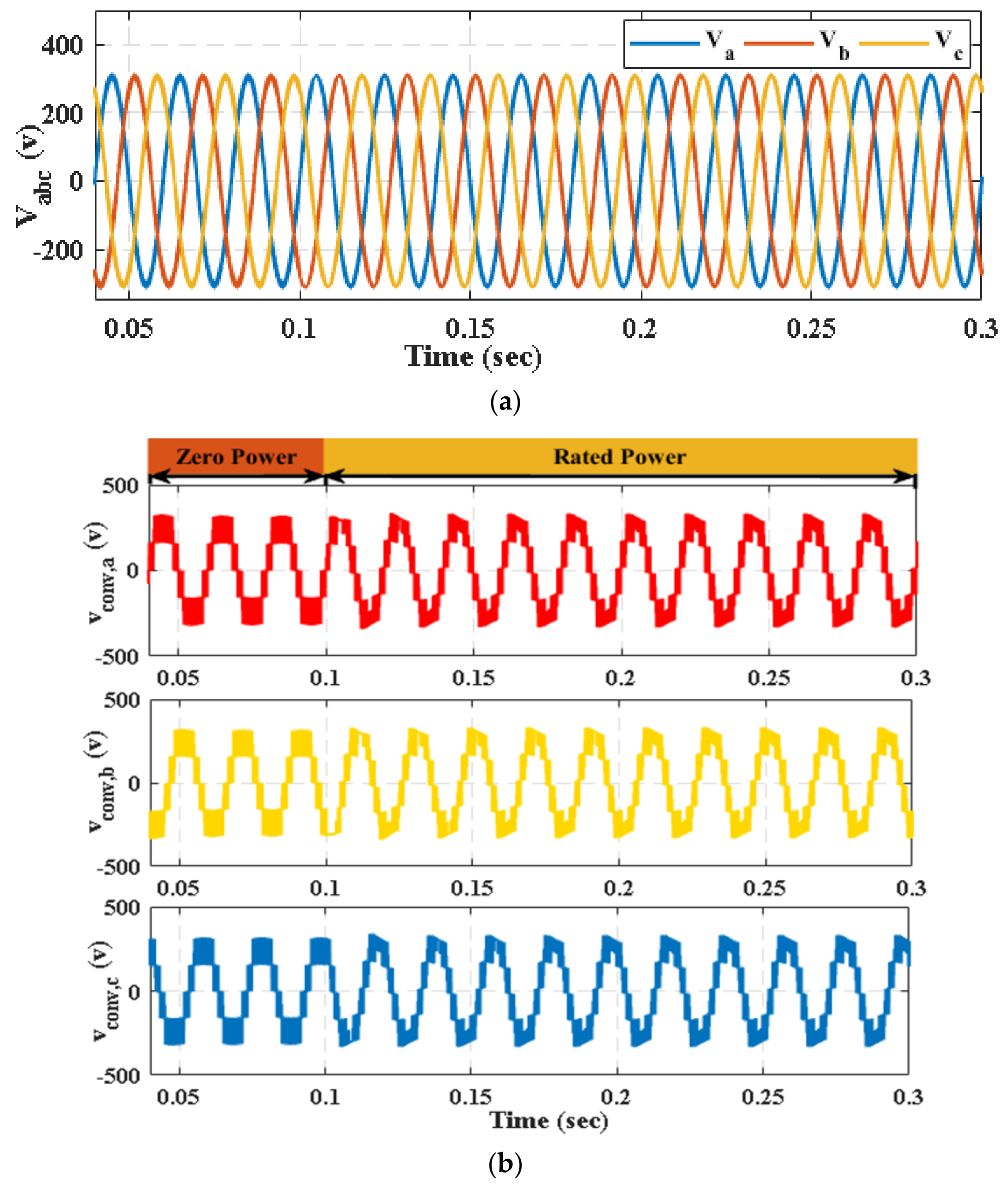
The grid voltage and converter output voltage are depicted in Figure 16. The gird voltage is shown in Figure 16a, while Figure 16b shows the five-level converter output voltage. The converter voltage shows a constant peak in zero power mode as the capacitor holds the energy in this mode since no power is transferring to the grid. In rated power mode, this is a slight variation in peak, as it is known that capacitor voltage is prone to variation. However, in conclusion, the waveform shows the good modulation and operation of MMC based on the proposed control scheme.

5. Conclusions

The theoretical analysis in this paper indicates that by transforming arm current to SRF and choosing a proper reference signal, the output current can be controlled as desired, and the circulating current can also be regulated to DC value. This will cause the suppression of the second harmonic component. The theoretical finding is validated using MATLAB simulation of five-level MMC. The results show a well-regulated output signal with THD (2.86%), which fulfills the criteria of the IEEE standard, and the circulating is also free of the second harmonic component. Furthermore, the capacitor voltage is also regulated to its means value. Moreover, both upper- and lower-arm current controllers are tuned with the same value, which makes the tuning easy. The results are compared with conventional leg-level controller graphically, and its performance indices are also calculated, which show a remarkable difference.