
A Cascade Proportional Integral Derivative Control for a Plate-Heat-Exchanger-Based Solar Absorption Cooling System


Abstract
:1. Introduction
2. Absorption Cooling System ACS
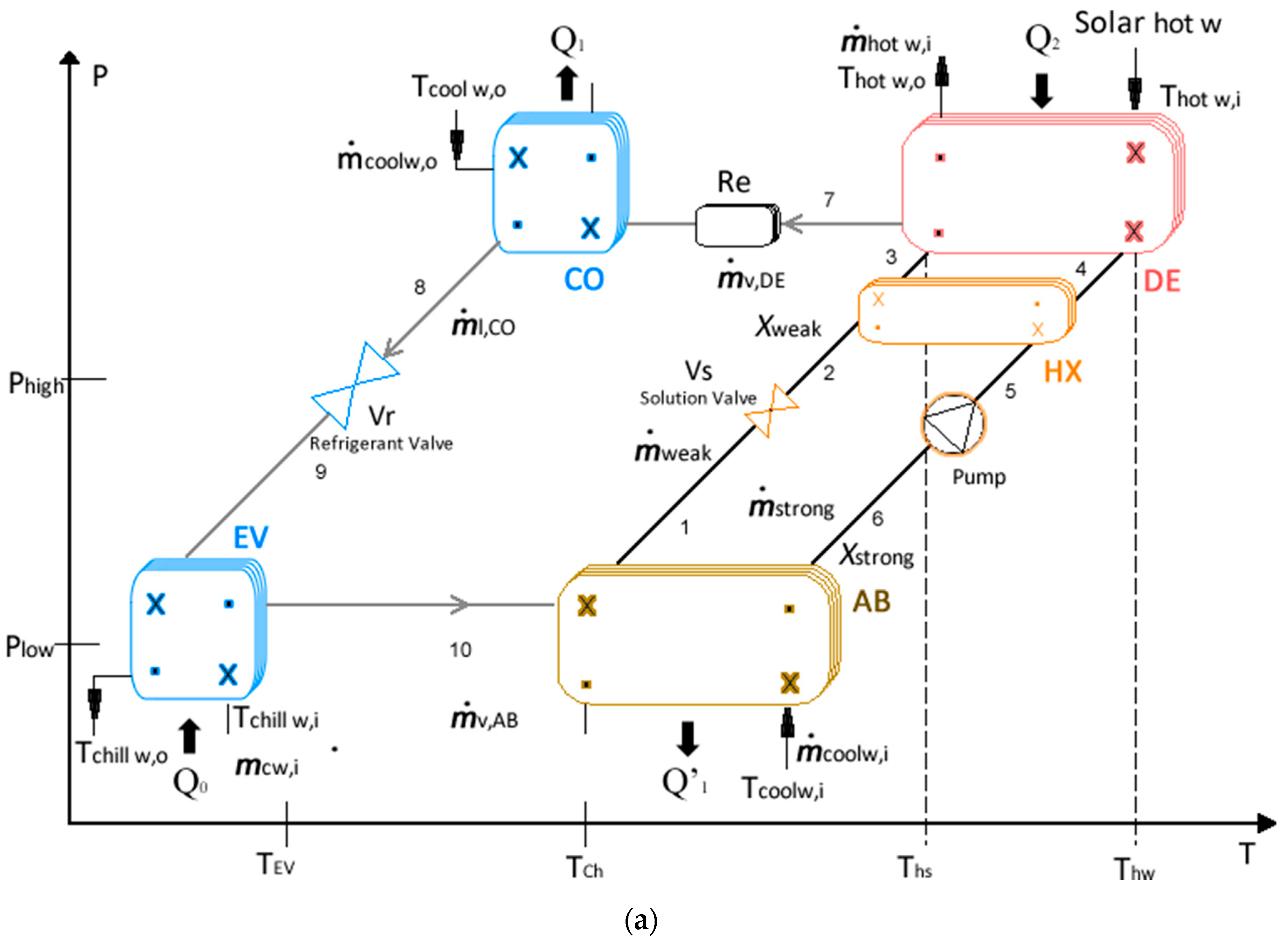
2.1. Main System
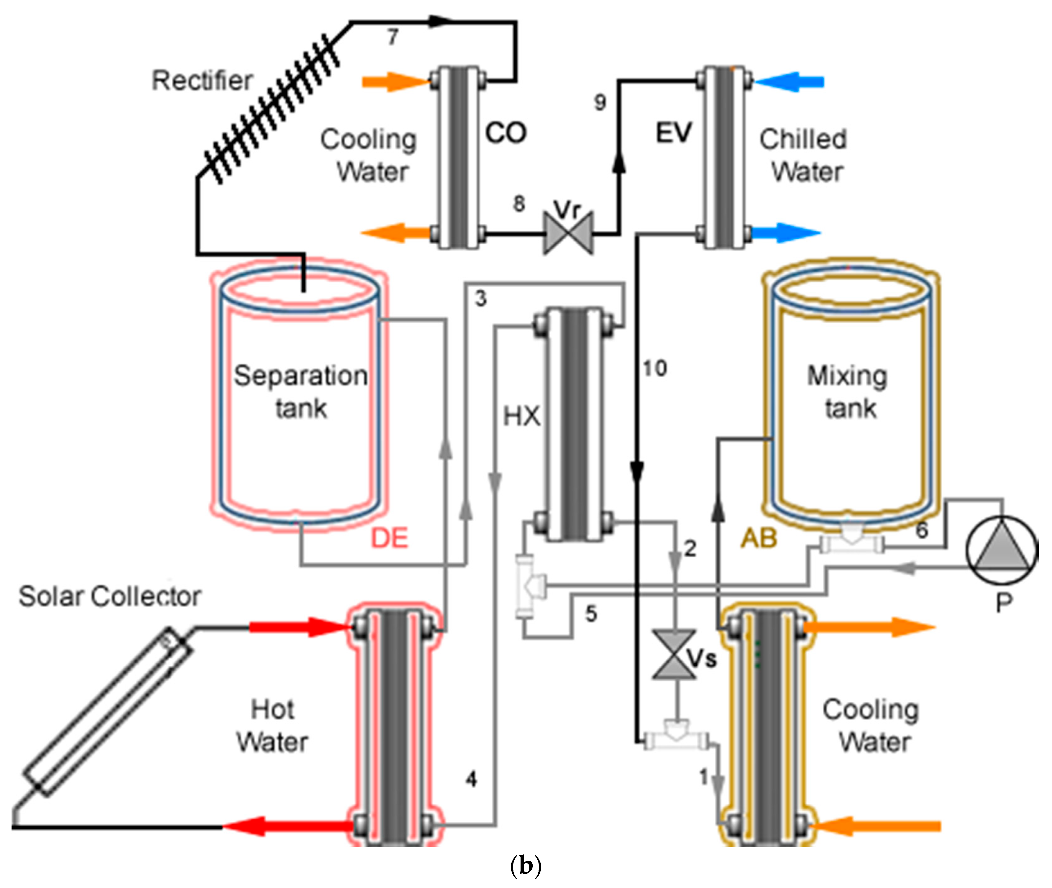
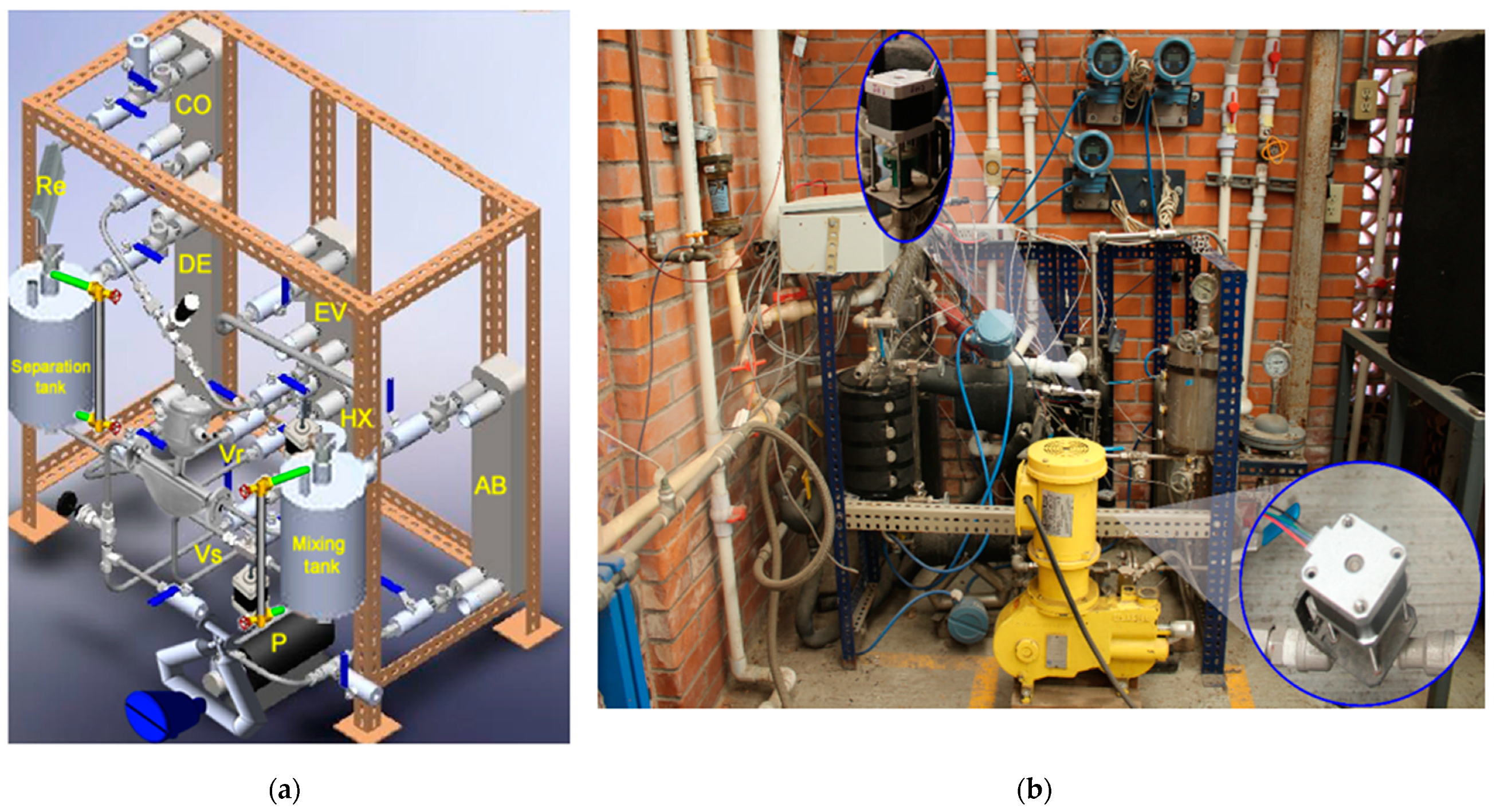
2.2. Experimental System
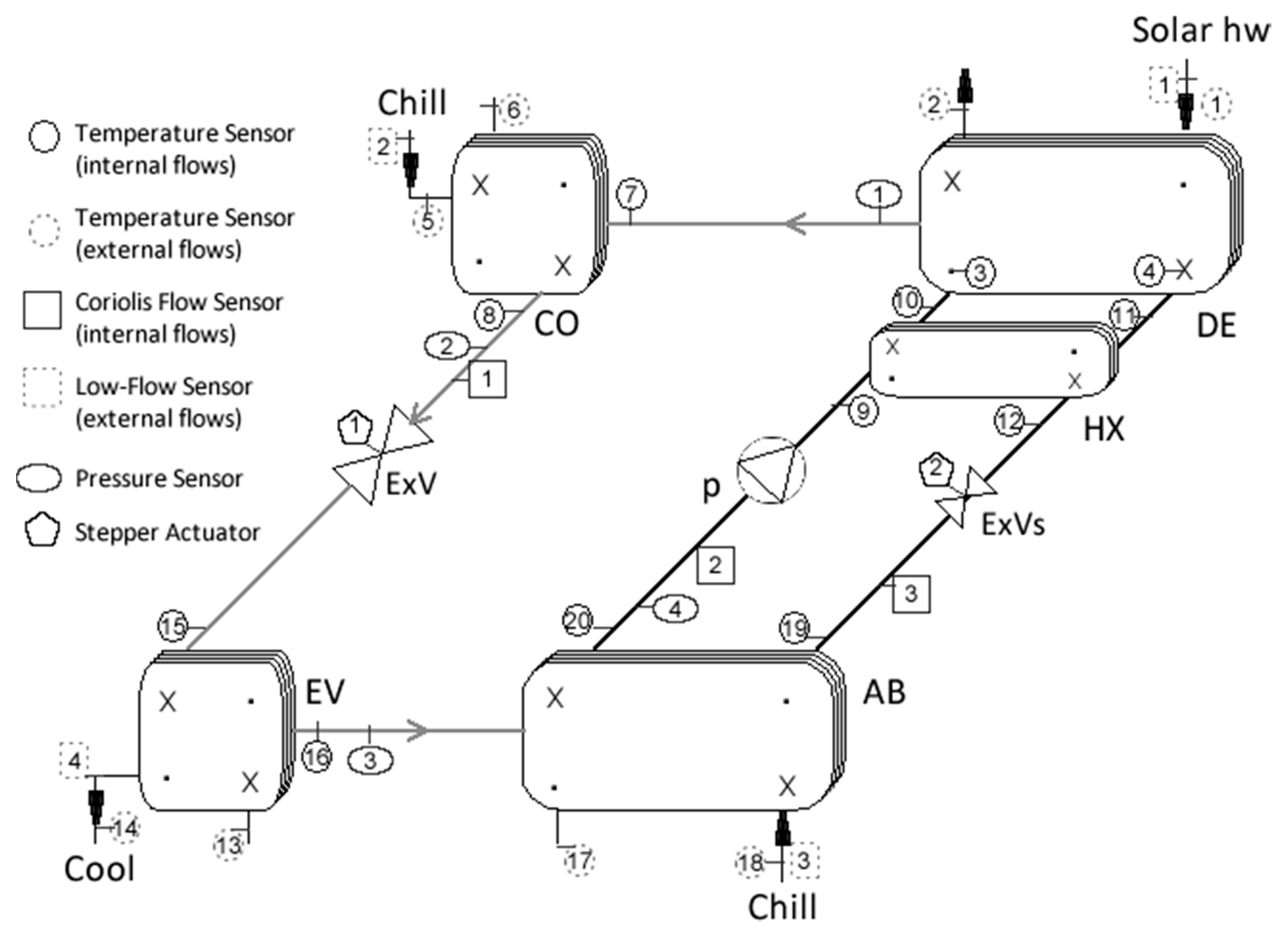
2.3. Dynamic System
- Only two pressures are considered: high (desorber–condenser) and low (absorber-evaporator);
- The thermal storage of the plates heat exchanger are neglected;
- There is no pressure loss in the pipes;
- The throttling process is isenthalpic;
- Heat transfer to and from the surroundings are ignored;
- The amount of work given to the pump is negligible;
- The fluid leaves each component at the component temperature;
- Constant heat exchanger efficiency.
3. Control System
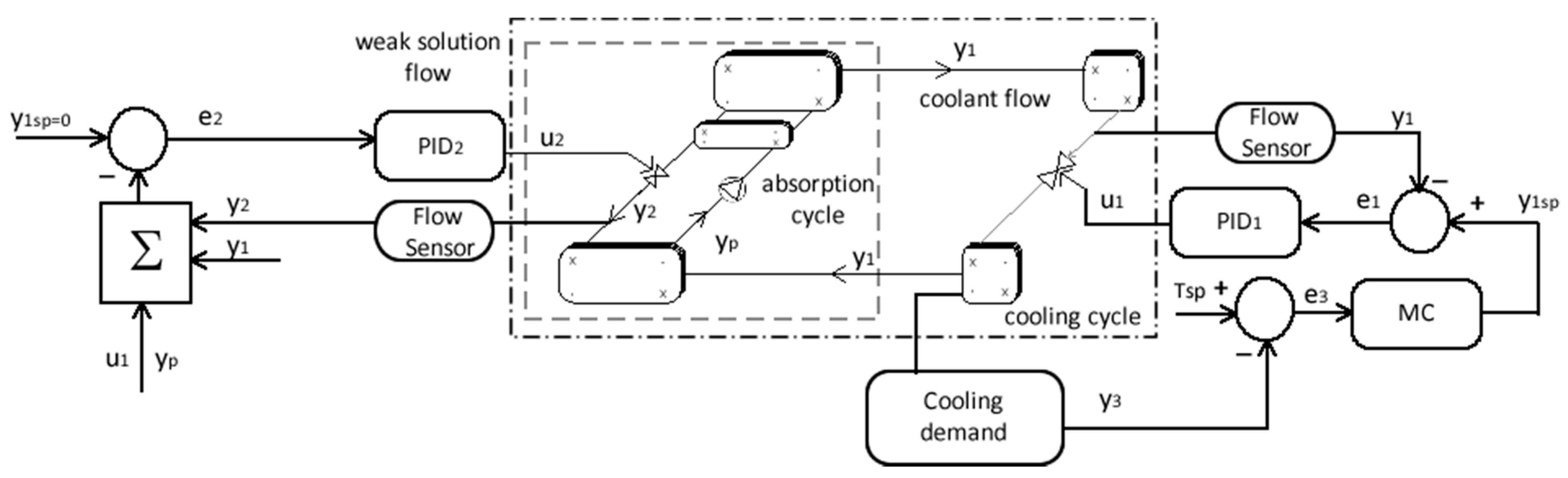
3.1. PID Control
3.2. PID Setup
4. Results
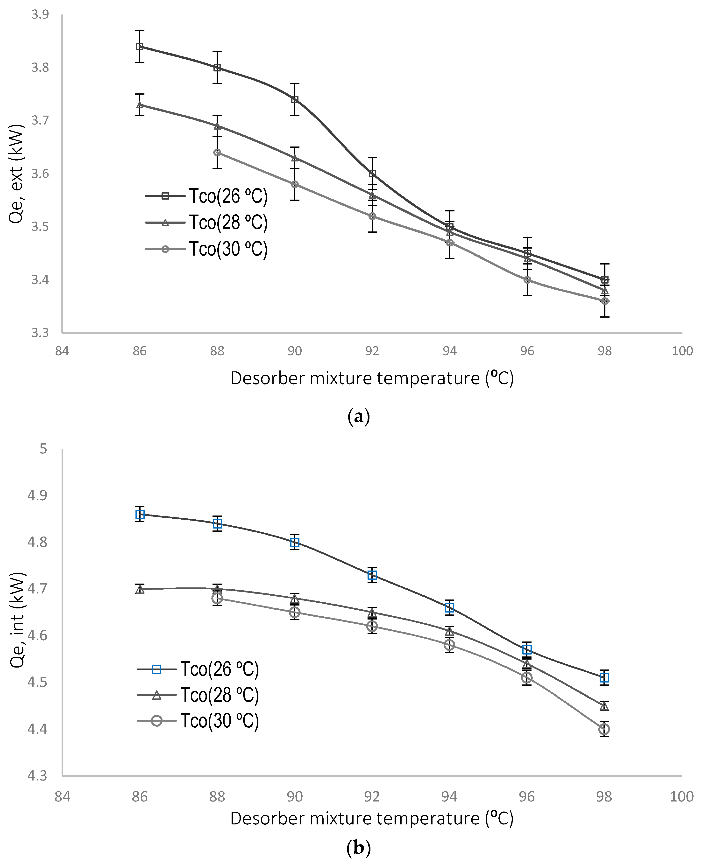
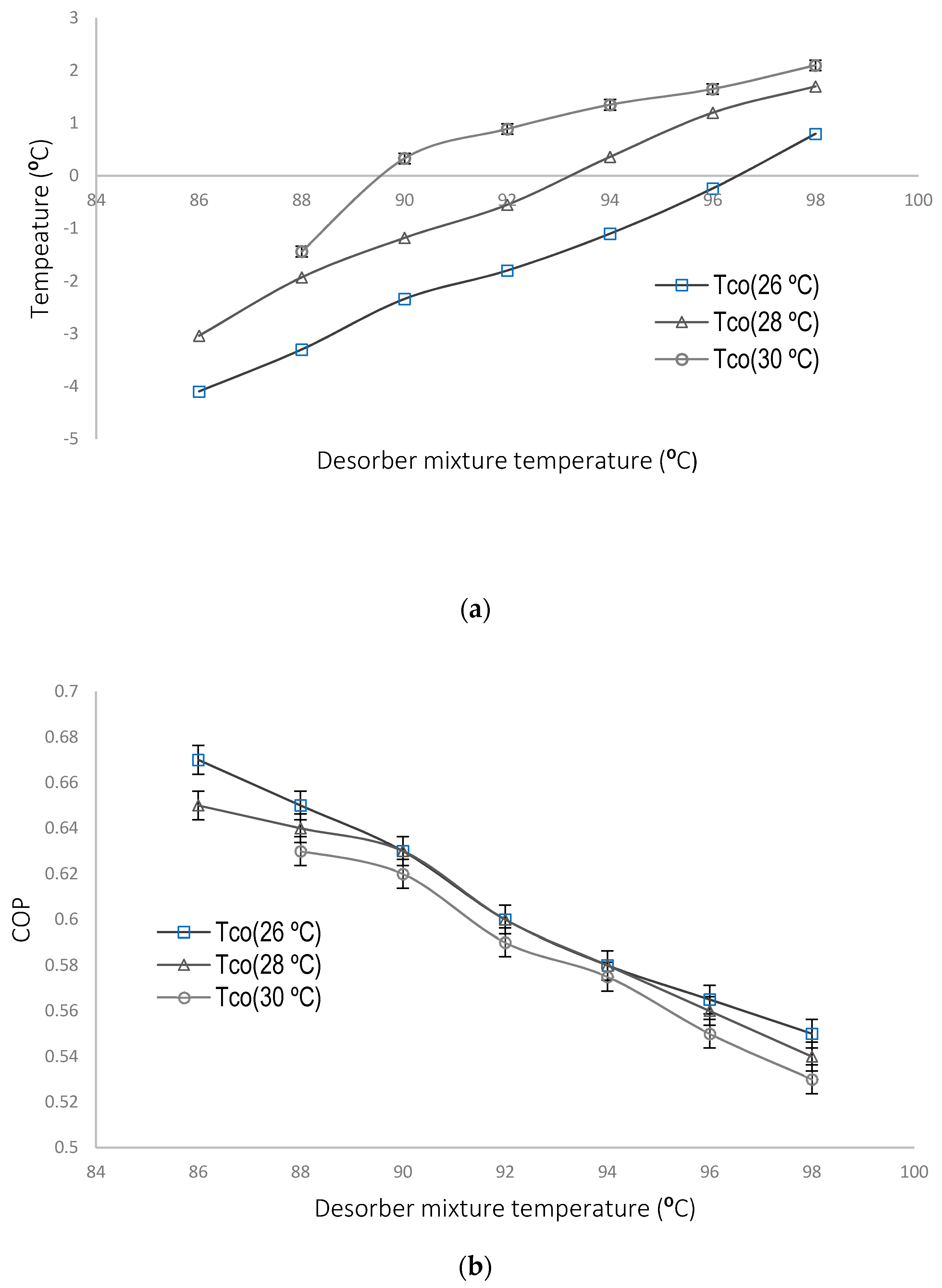
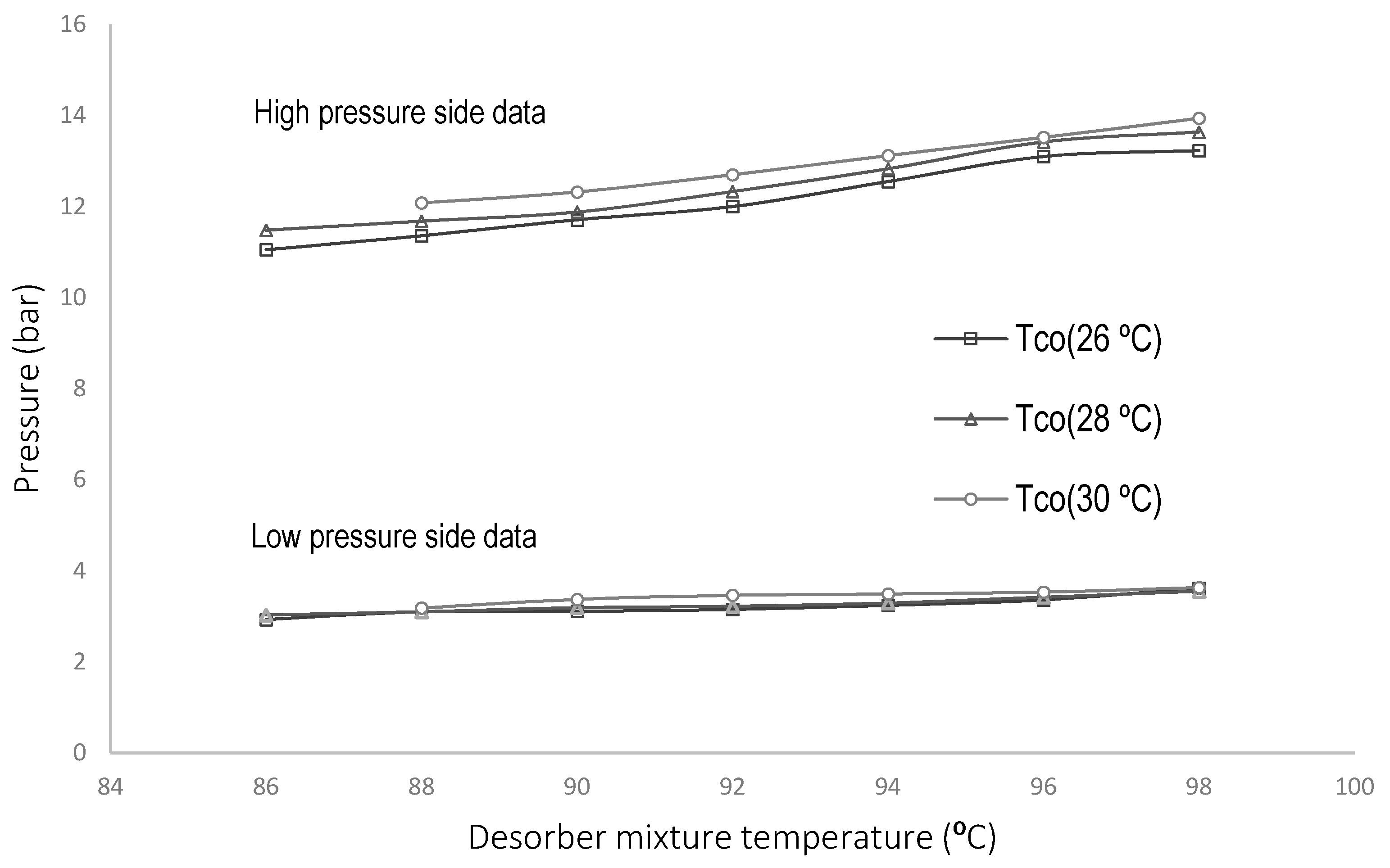
4.1. Parametric Evaluation of the Experimental System
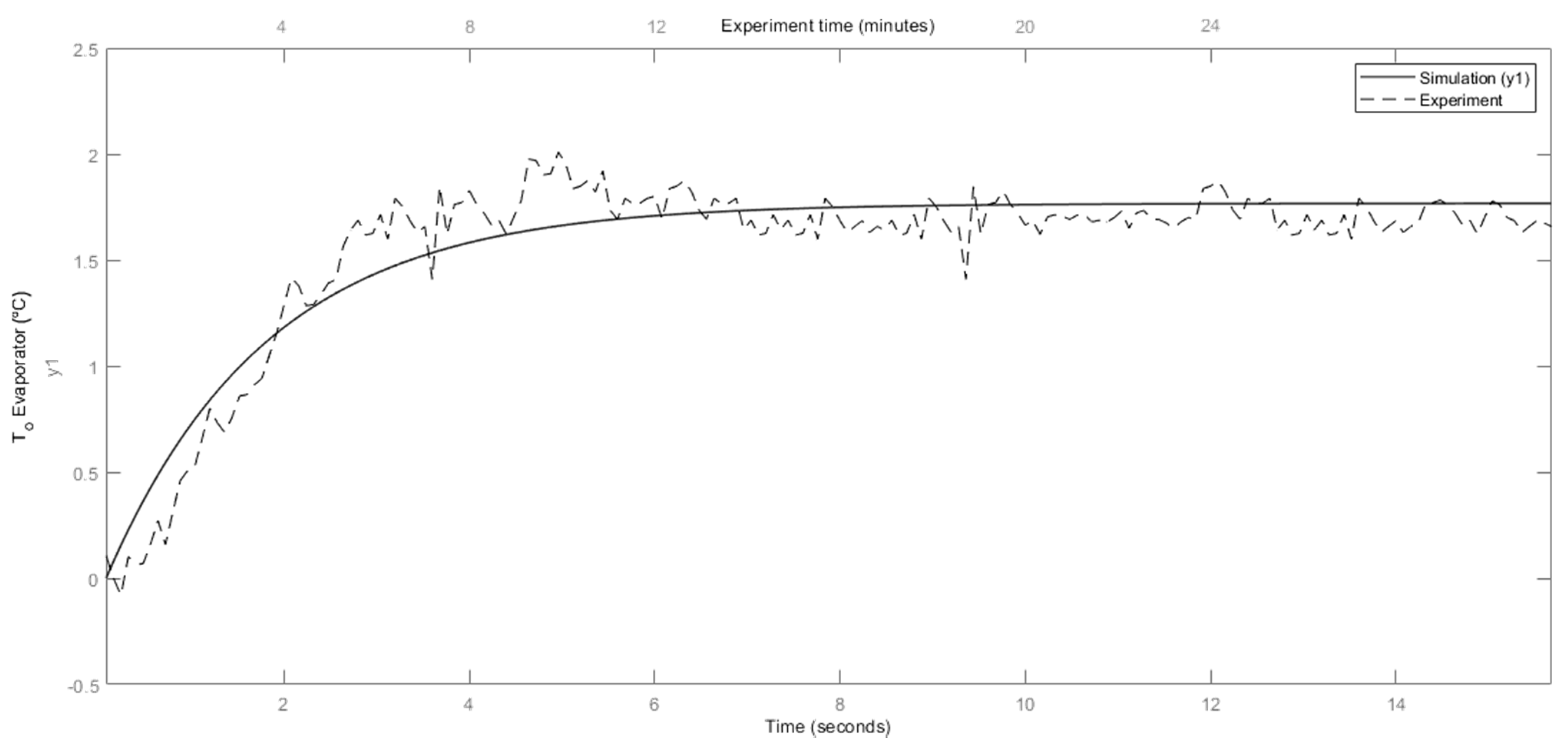
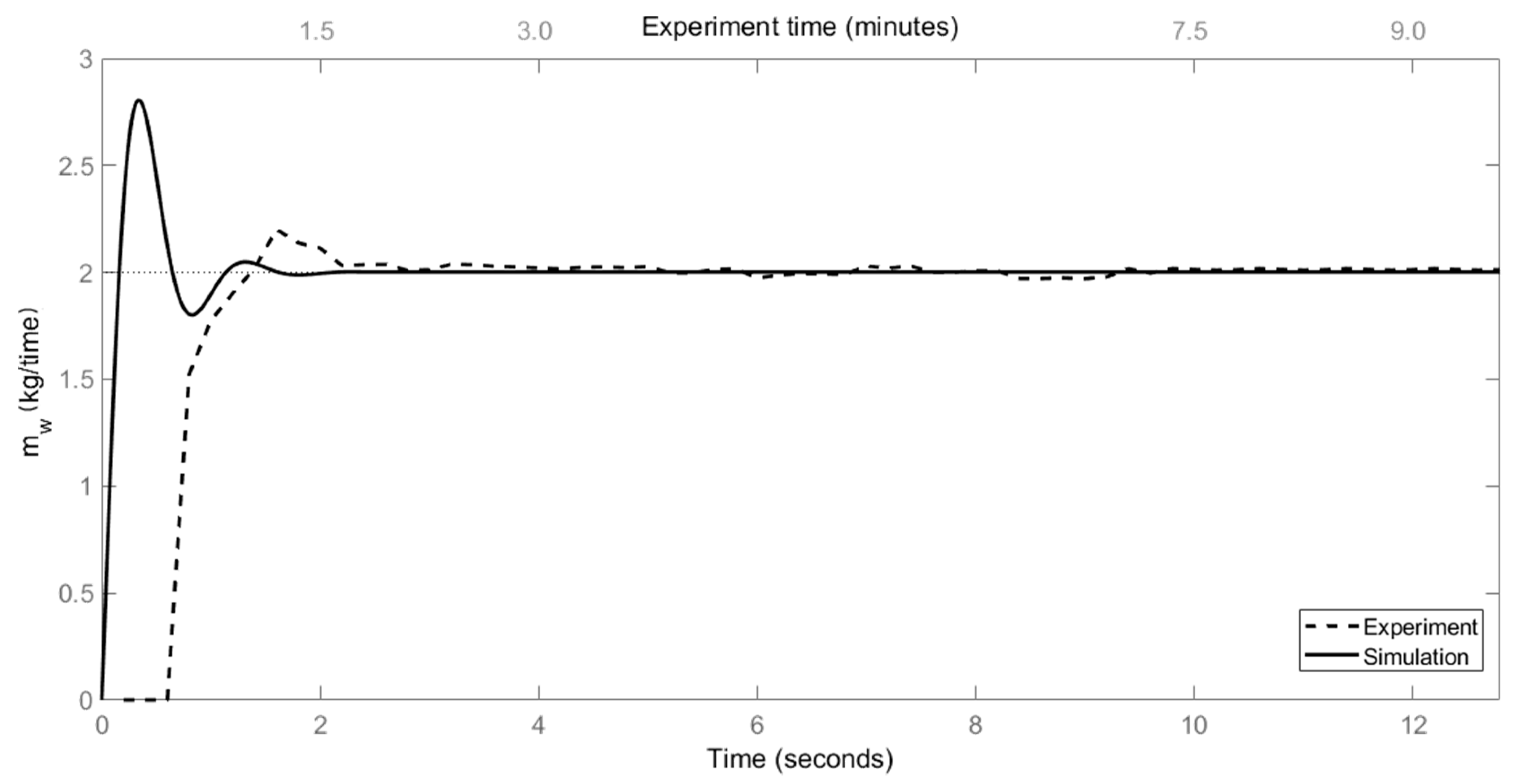
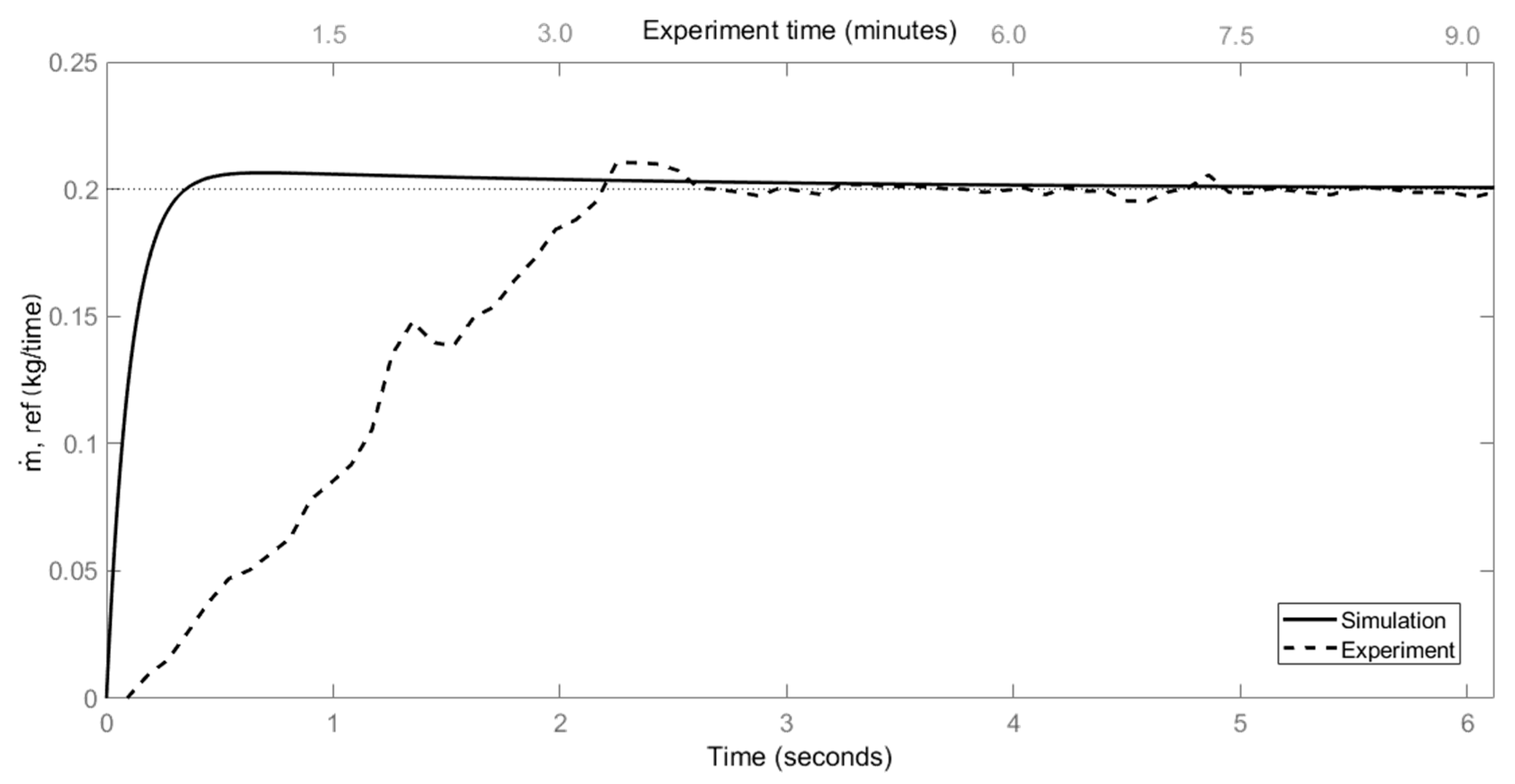
4.2. Dynamic Model
4.3. PID Control
5. Discussion
6. Conclusions
Author Contributions
Funding
Institutional Review Board Statement
Informed Consent Statement
Data Availability Statement
Acknowledgments
Conflicts of Interest
Nomenclature
| A | effective area in contact (m2) |
| minimum cross-section area (m2) | |
| AB | absorber |
| CO | condenser |
| COP | coefficient of performance |
| Cp | specific heat at constant pressure (kJ/kg–K) |
| flow coefficient of the valve | |
| DE | desorber |
| EV | evaporator |
| FR | flow ratio |
| HX | heat exchanger |
| H | specific enthalpy (kJ/kg) |
| mass flow (kg/min) | |
| M | mass (kg) |
| P | solution pump |
| heat rate (kW) | |
| R | refrigeration |
| RE | rectifier |
| T | temperature (°C) |
| T | time (s) |
| U | heat transfer coefficient (kW/m2K) |
| UA | global thermal surface conductivity (kW/K) |
| Vr | refrigerant expansion throttle valve |
| Vs | solution expansion throttle valve |
| W | power (kW) |
| X | concentration of the NH3H2O solution |
| Z | height difference between the upper component outlet and lower component inlet |
| Z | proportion level height of liquid in the upper component to the accumulative mass |
| Subscript: | |
| 0 | ambience |
| chill w | chilled water |
| cool w | cooling water |
| hot s | hot solution |
| hot w | hot water |
| i, o | inlet, outlet |
| l | liquid phase |
| max | maximum |
| p | pump |
| r | refrigerant |
| s | solution |
| strong | strong solution |
| v | vapor phase |
| vl | valve |
| weak | weak solution |
References
- IEA-Cooling. Tracking Report-June 2020. Available online: https://www.iea.org/reports/cooling (accessed on 1 June 2021).
- Kalkan, N.; Young, E.A.; Celiktas, A. Solar thermal air conditioning technology reducing the footprint of solar thermal air conditioning. Renew. Sust. Energy Rev. 2012, 16, 6352–6383. [Google Scholar] [CrossRef]
- Joudi, K.A.; Lafta, A.H. Simulation of a simple absorption refrigeration system. Energy Convers. Manag. 2001, 42, 1575–1605. [Google Scholar] [CrossRef]
- Ziegler, F. Recent developments and future prospects of sorption heat pump systems. Int. J. Therm. Sci. 1999, 38, 191–208. [Google Scholar] [CrossRef]
- Ziegler, F.; Alefeld, G. Coefficient of performance of multistage absorption cycles. Int. J. Refrig. 1987, 10, 285–295. [Google Scholar] [CrossRef]
- Ziegler, J.G.; Nichols, N.B. Optimum settings for automatic controllers. Math. Comput. Sci. 1942, 64, 759–768. [Google Scholar] [CrossRef]
- Labus, J.M.; Bruno, C.J.; Coronas, A. Review on absorption technology with emphasis on small capacity absorption machines. J. Therm. Sci. Eng. Appl. 2013, 17, 739–762. [Google Scholar] [CrossRef]
- Abed, A.M.; Alghoul, M.A.; Sopiana, K.; Majdi, H.S.; Al-Shamani, A.N.; Muftah, A.F. Enhancement aspects of single stage absorption cooling cycle: A detailed review. Renew. Sust. Energy Rev. 2017, 77, 1010–1045. [Google Scholar] [CrossRef]
- Srikhirin, P.; Aphornratana, S.; Chungpaibulpatana, S. A review of absorption refrigeration technologies. Renew. Sust. Energy Rev. 2001, 5, 343–372. [Google Scholar] [CrossRef]
- Dincer, I.; Midilli, A.; Hepbasli, A.; Karakoc, T.H. Global Warming: Engineering Solutions; Springer: Boston, MA, USA, 2010; pp. 147–159. [Google Scholar]
- Dincer, I.; Dost, D. A simple model for heat and mass transfer in absorption cooling systems (ACSs). Int. J. Energy Res. 1996, 20, 237–243. [Google Scholar] [CrossRef]
- Ng, K.C.; Chua, H.T.; Han, Q.; Kashiwagi, T.; Akisawa, A.; Tsurusawa, T. Thermodynamic Modeling of Absorption Chiller and Comparison with Experiments. Heat Transf. Eng. 1999, 20, 42–51. [Google Scholar]
- Sterner, D.; Sunden, B. Performance of plate heat exchangers for evaporation of ammonia. Heat Transf. Eng. 2006, 27, 45–55. [Google Scholar] [CrossRef]
- Goodarzi, M.; Amiri, A.; Mohammad, S.G.; Mohammad, R.S.; Kirimipour, A.; Languri, E.M.; Dahari, M. Investigation of heat transfer and pressure drop of a counter flow corrugated plate heat exchanger using MWCNT based nanofluids. Int. Commun. Heat Mass Transf. 2015, 66, 172–179. [Google Scholar] [CrossRef]
- Evola, G.; Le Pierrès, N.; Boudehenn, F.; Papillon, P. Proposal and validation of a model for the dynamic simulation of a solar-assisted single-stage LiBr/water absorption chiller. Int. J. Refrig. 2013, 36, 1015–1028. [Google Scholar] [CrossRef]
- Kim, B.; Park, J. Dynamic simulation of a single-effect ammonia-water absorption chiller. Int. J. Refrig. 2007, 30, 535–545. [Google Scholar] [CrossRef]
- Ruz, M.L.; Garrido, J.; Vázquez, F.; Morilla, F. A hybrid modeling approach for steady-state optimal operation of vapor compression refrigeration cycles. Appl. Therm. Eng. 2017, 120, 74–87. [Google Scholar] [CrossRef] [Green Version]
- Kim, D.S.; Infante Ferreira, C.A. Analytic modelling of steady state-single effect absorption cycles. Int. J. Refrig. 2008, 31, 1012–1020. [Google Scholar] [CrossRef]
- Cai, W.; Sen, M.; Paolucci, S. Dynamic simulation of an ammonia-water absorption refrigeration system. Ind. Eng. Chem. Res. 2011, 51, 2070–2076. [Google Scholar] [CrossRef]
- Viswanathan, V.K.; Rattner, A.S.; Determan, M.D.; Garimella, S. Dynamic model for a small-capacity ammonia-water absorption chiller. HVACR Res. 2013, 19, 865–881. [Google Scholar] [CrossRef]
- Martinho, L.C.S.; Vargas, J.V.C.; Balmant, W.; Ordonez, J.C. A single stage absorption refrigeration system dynamic mathematical modeling, adjustment and experimental validation. Int. J. Refrig. 2016, 68, 130–144. [Google Scholar] [CrossRef]
- Iranmanesh, A.; Mehrabian, A.M. Dynamic simulation of a single-effect LiBr-H2O absorption refrigeration cycle considering the effects of thermal masses. Energy Build. 2013, 60, 47–59. [Google Scholar] [CrossRef]
- Ochoa, A.A.V.; Dutra, J.C.C.; Henríquez, J.R.G.; dos Santos, C.A.C. Dynamic study of a single effect absorption chiller using the pair LiBr/H2O. Energy Convers. Manag. 2016, 108, 30–42. [Google Scholar] [CrossRef]
- Kohlenbach, P.; Ziegler, F. A dynamic simulation model for transient absorption chiller performance. Part II: Numerical results and experimental verification. Int. J. Refrig. 2008, 31, 226–233. [Google Scholar] [CrossRef]
- Puig-Arnavat, M.; López-Villada, J.; Bruno, J.C.; Coronas, A. Analysis and parameter identification for characteristic equations of single- and double-effect absorption chillers by means of multivariable regression. Int. J. Refrig. 2010, 33, 70–78. [Google Scholar] [CrossRef]
- Albers, J.; Kühn, A.; Petersen, S.; Ziegler, F. Control of Absorption Chillers by Insight: The characteristic equation. Czas. Tech. Mech. 2008, 105, 3–12. [Google Scholar]
- Albers, J. New absorption chiller and control strategy for the solar assisted cooling system at the German federal environment agency. Int. J. Refrig. 2014, 39, 48–56. [Google Scholar] [CrossRef]
- Matsushima, H.; Fujii, T.; Komatsu, T.; Nishiguchi, A. Dynamic simulation program with object-oriented formulation for absorption chillers (modelling, verification, and application to triple-effect absorption chiller). Int. J. Refrig. 2010, 33, 259–268. [Google Scholar] [CrossRef]
- Yao, Y.; Huang, M.; Chen, J. State-space model for dynamic behavior of vapor compression liquid chiller. Int. J. Refrig. 2013, 36, 2128–2147. [Google Scholar] [CrossRef]
- Osta-Omar, S.M.; Micallef, C. Mathematical Model of a Lithium-Bromide/Water Absorption Refrigeration System Equipped with and Adiabatic Absorber. Computation 2016, 4, 44. [Google Scholar] [CrossRef] [Green Version]
- Wen, H.; Wu, A.; Liu, Z.; Shang, Y. A State-Space Model for Dynamic Simulation of a Single-Effect LiBr/H2O Absorption Chiller. IEEE Access 2019, 7, 57251–57258. [Google Scholar] [CrossRef]
- Fernández-Seara, J.; Vázquez, M. Study and control of the optimal generation temperature in NH3-H2O absorption refrigeration system. Appl. Therm. Eng. 2001, 21, 343–357. [Google Scholar] [CrossRef]
- Rêgo, A.T.; Hanriot, S.M.; Oliveira, A.F.; Brito, P.; Rêgo, T.F.U. Automotive exhaust gas flow control for an ammonia-water absorption refrigeration system. Appl. Therm. Eng. 2014, 64, 101–107. [Google Scholar] [CrossRef]
- Jeong, A.S.; Younggy, S.; Chung, J.D. Dynamics and control of solution levels in a high temperature generator for an absorption chiller. Int. J. Refrig. 2012, 35, 1123–1129. [Google Scholar]
- Güido, W.H.; Lanser, W.; Petersen, S.; Ziegler, F. Performance of absorption chillers in field test. Appl. Therm. Eng. 2018, 134, 353–359. [Google Scholar] [CrossRef]
- Bennet, S. The Past of PID Controllers. Annu. Rev. Control 2001, 25, 43–53. [Google Scholar] [CrossRef]
- Björn, N.; Dalibard, A.; Schnabel, L.; Eicker, U. Approaches for the optimized control of solar thermally driven cooling systems. Appl. Energy 2017, 185, 732–744. [Google Scholar]
- Sabbagh, A.A.; Gómez, J.M. Optimal control of single stage LiBr/water absorption chiller. Int. J. Refrig. 2018, 92, 1–9. [Google Scholar] [CrossRef]
- Hamid, N.; Kamal, M.; Yahaya, F.H. Application of PID controller in controlling refrigerator temperature. In Proceedings of the 2009 5th International Colloquium on Signal Processing & Its Applications, Kuala Lumpur, Malaysia, 6–8 March 2009; Volume 1, pp. 378–384. [Google Scholar]
- Salazar, M.; Méndez, F. PID control for a single-stage transcritical CO2 refrigeration cycle. Appl. Therm. Eng. 2014, 67, 429–438. [Google Scholar] [CrossRef]
- Bejarano, G.; Alfaya, J.A.; Rodriguez, D.; Morilla, F.; Ortega, M.G. Benchmark for PID control of Refrigeration Systems based on Vapour Compression. IFAC Pap. 2018, 51, 497–502. [Google Scholar] [CrossRef]
- Zadeh, L.A. Fuzzy Sets. Inf. Control 1965, 8, 338–353. [Google Scholar] [CrossRef] [Green Version]
- Visek, E.; Mazzrella, L.; Motta, M. Performance Analysis of a Solar Cooling System Using Self-Tuning Fuzzy-PID Control with TRNSYS. Energy Procedia 2014, 57, 2609–2618. [Google Scholar] [CrossRef] [Green Version]
- Lima, K.C.; Caldas, A.M.A.; dos Santos, C.A.C.; Ochoa, A.A.V.; Dutra, J.C.C. Flow Control For Absorption Chillers Using the Par LiBr/H2O Driven in Recirculation Pumps of Low Power. IEEE Access 2016, 14, 1624–1629. [Google Scholar] [CrossRef]
- Vinther, K.; Nielsen, R.J.; Nielsen, K.M.; Andersen, P.; Pedersen, T.S.; Bendtsen, J.D. Absorption Cycle Heat Pump Model for Control Design. In Proceedings of the 2015 European Control Conference (ECC), Linz, Austria, 15–17 July 2015. [Google Scholar]
- Jiménez-García, J.C.; Rivera, W. Parametric analysis on the experimental performance of an ammonia/water absorption cooling system built with plate heat exchangers. Appl. Therm. Eng. 2019, 148, 87–95. [Google Scholar] [CrossRef]
- Hewitt, N.J.; Mcmullan, J.T.; Murphy, N.E.; Ng, C.T. Comparison of expansion valve performance. Int. J. Energy Res. 1995, 19, 347–359. [Google Scholar] [CrossRef]
- Tassou, S.A.; Al-Nizari, H.O. Investigation of the effects of thermostatic and electronic expansion valves on the steady-state and transient performance of commercial chillers. Int. J. Refrig. 1993, 16, 49–56. [Google Scholar] [CrossRef]
- Shinskey, F.G. Process Control Systems: Application, Design, and Tuning, 4th ed.; McGraw-Hill Inc.: New York, NY, USA, 1996; pp. 74–79. [Google Scholar]
- Tillner-Roth, R.; Friend, D.G. A Helmholtz Free Energy Formulation of the Thermodynamic Properties of the Mixture {Water + Ammonia}. J. Phys. Chem. Ref. Data 1998, 27, 63–96. [Google Scholar] [CrossRef] [Green Version]
- Iso GUM. Guide to the Expression of Uncertainty in Measurementm; ISO: Geneva, Switzerland, 2008. [Google Scholar]
- Moffat, R.J. Using Uncertainty Analysis in the Planning of an Experiment. J. Fluids Eng. 1985, 107, 173–178. [Google Scholar] [CrossRef]
- Moffat, R.J. Contributions to the Theory of Single-Sample Uncertainty Analysis. J. Fluids Eng. 1982, 104, 250–258. [Google Scholar] [CrossRef] [Green Version]


| Variable | Measuring Instrument | Operation Range | Accuracy |
|---|---|---|---|
| Flow | Coriolis flow meter | 0 to 20 (kg/min) | ±0.1% |
| Impeller flow meter | 0 to 60 (kg/min) | ±1% | |
| Pressure | Pressure transductor | 0 to 25 (bar) | ±1% |
| Temperature | RTD temperature | −40 a 750 (°C) | ±0.3 °C |
| Parameters | Units | Experimental Value |
|---|---|---|
| Pressures | ||
| Desorber | bar | 11–15 |
| Condenser | bar | 10–14 |
| Evaporator | bar | 2–4 |
| Absorber | bar | 2–3 |
| Flow rates | ||
| Refrigerant | kg/min | 0.1–0.3 |
| Chilled water | kg/min | 10 |
| Cooling water | kg/min | 20 |
| Hot water | kg/min | 16 |
| Temperatures | ||
| Chilled water inlet EV | °C | 25–20 |
| Cooling water inlet CO, AB | °C | 26–30 |
| Heating water inlet DE | °C | 98–110 |
| Inlet condenser | °C | 90–100 |
| Outlet condenser | °C | 30–32 |
| Inlet evaporator | °C | 24–26 |
| Outlet evaporator | °C | −4–2 |
| Inlet desorber | °C | 90–100 |
| Ammonia concentrations | ||
| Weak solution NH3 fraction | 16.86–17.15 | |
| Strong solution NH3 fraction | 38.22–41.11 | |
| Refrigerant NH3 fraction | 99.21 | |
| Cycle external performance | ||
| COP | 0.56–0.61 | |
| QEV | kW | 3.1–3.9 |
| QDE | kW | 5.8–6.8 |
| QCO | kW | 4.0–4.5 |
| QAB | kW | 4.5–5.5 |
| Symbol | Description | Value |
|---|---|---|
| Hot water mass flow rate (kg/min) | 16 | |
| Cooling water mass flow rate(kg/min) | 10 | |
| Chilled water mass flow rate (kg/min) | 15 | |
| Solution pump frequency (Hz) | 60 | |
| Inlet hot water temperature (°C) | 95–110 | |
| Inlet cooling water temperature (°C) | 26 | |
| Inlet chilled water temperature (°C) | 26–30 | |
| Strong solution mass flow rate (kg/min) | 2 | |
| Initial NH3 concentration in the mixture (%) | 40 |
| Symbol | Description | Value |
|---|---|---|
| Overall mass of NH3 (kg) | 4 | |
| Overall mass of NH3 and H2O (kg) | 10 | |
| Desorber heat transfer coefficient (kW/K) | 1.35 | |
| Condenser heat transfer coefcient (kW/K) | 3.36 | |
| Evaporator heat transfer coefficient (kW/K) | 2.43 | |
| Absorber heat transfer coefficient (kW/K) | 1.9 | |
| DE–AB height differee (m) | 0.06 | |
| DE–AB height difference (m) | 0.2 | |
| Solution heat exchanger coefficient (-) | 0.4 |
| Type | C0 | C1 | C2 | C3 |
|---|---|---|---|---|
| 0.8 | 0.6 | 0.4 | 0.4 | |
| 0.6 | 0.3 | 0.15 | 0.25 | |
| 0.25 | 0.1 | 0.0 | 0.0 | |
| 0.6 | 0.4 | 0.3 | 0.36 | |
| 0.6 | 0.4 | 0.3 | 0.25 | |
| 0.5 | 0.2 | 0.0 | 0.1 |
Publisher’s Note: MDPI stays neutral with regard to jurisdictional claims in published maps and institutional affiliations. |
© 2021 by the authors. Licensee MDPI, Basel, Switzerland. This article is an open access article distributed under the terms and conditions of the Creative Commons Attribution (CC BY) license (https://creativecommons.org/licenses/by/4.0/).
Share and Cite
Garcíadealva, Y.; Best, R.; Gómez, V.H.; Vargas, A.; Rivera, W.; Jiménez-García, J.C. A Cascade Proportional Integral Derivative Control for a Plate-Heat-Exchanger-Based Solar Absorption Cooling System. Energies 2021, 14, 4058. https://doi.org/10.3390/en14134058
Garcíadealva Y, Best R, Gómez VH, Vargas A, Rivera W, Jiménez-García JC. A Cascade Proportional Integral Derivative Control for a Plate-Heat-Exchanger-Based Solar Absorption Cooling System. Energies. 2021; 14(13):4058. https://doi.org/10.3390/en14134058
Chicago/Turabian StyleGarcíadealva, Yeudiel, Roberto Best, Víctor Hugo Gómez, Alejandro Vargas, Wilfrido Rivera, and José Camilo Jiménez-García. 2021. "A Cascade Proportional Integral Derivative Control for a Plate-Heat-Exchanger-Based Solar Absorption Cooling System" Energies 14, no. 13: 4058. https://doi.org/10.3390/en14134058
APA StyleGarcíadealva, Y., Best, R., Gómez, V. H., Vargas, A., Rivera, W., & Jiménez-García, J. C. (2021). A Cascade Proportional Integral Derivative Control for a Plate-Heat-Exchanger-Based Solar Absorption Cooling System. Energies, 14(13), 4058. https://doi.org/10.3390/en14134058