Method for Determining the Utilization Rate of Thin-Deck Shearers Based on Recorded Electromotor Loads

Abstract

Mining machinery and equipment used in modern mining are equipped with sensors and measurement systems at the stage of their production. Measuring devices are most often components of a control system or a machine performance monitoring system. In the case of headers, the primary task of these systems is to ensure safe operation and to monitor its correctness. It is customary to collect information in very large databases and analyze it when a failure occurs. Data mining methods allow for analysis to be made during the operation of machinery and mining equipment, thanks to which it is possible to determine not only their technical condition but also the causes of any changes that have occurred. The purpose of this work is to present a method for discovering missing information based on other available parameters, which facilitates the subsequent analysis of machine performance. The primary data used in this paper are the currents flowing through the windings of four header motors. In the method, the original reconstruction of the data layout was performed using the R language function, and then the analysis of the operating states of the header was performed based on these data. Based on the rules used and determined in the analysis, the percentage structure of machine operation states was obtained, which allows for additional reporting and verification of parts of the process.

1. Introduction

The continuously growing demand for electricity in the world encourages the rational use of energy resources. The extraction of hard coal from thin seams is one of the possibilities for the rational management of natural resources, particularly in those countries where the deposits that are the most attractive in terms of extraction profitability, i.e., those located in medium and thick seams, have already been partially or completely mined. In recent years, the coal reserve of medium-thick and thick coal seams, which are thicker than 2 m, has decreased significantly [1].

Since no available energy source can be ignored, the possibility of the economically viable exploitation of thin deposits has received increasing attention in recent years [2,3,4]. Satisfactory technical and economic results are possible to obtain with the use of fully mechanized equipment [5].

In some countries, it is assumed that the lower limit of deposit thickness for thin seams is 0.4–0.5 m. In Ukrainian coal mining, the assumed thickness is 0.7–1.2 m [6,7,8], with a lower technical limit of 0.65 m [9]. In Chinese conditions, thin seams are those with a thickness of 0.8–1.3 m, while seams thinner than 0.8 m are classified as extremely thin [10]. In the case of Poland, thin seams are those with a thickness of 1–1.5 m.

The exploitation of thin seams is a point of focus not only for users but also for mining machinery manufacturers. Decades of efforts resulted in significant achievements, and the automation level of thin coal seam mining has been gradually improving. Currently, longwall shearers or static coal plows are most commonly used to mine thin seams. Their advantages, disadvantages, and adaptability for different geological conditions can be found in the literature [11,12]. A longwall shearer is a component of a mechanized longwall system that is also equipped with a face conveyor and powered roof support. The mechanized longwall system enables the execution of the mining process and the loading and haulage of the excavated material from the longwall. Currently, regardless of the thickness of the seam, the most popular of the produced mining machines are two-arm, two-unit shearers moving on the conveyor by means of a chainless haulage system. A unique solution used for two-way, noncavity mining and loading of coal in thin seams is the Mikrus system, which is equipped with a GUŁ-500 mining and loading head. The data used for this study were acquired from the Mikrus system, for the period in which the shearer was tested under actual working conditions.

The use of the right mining machines for mining low seams is crucial to an efficient coal mining process. The possibility of obtaining relevant data from them is also important. The intensive digitization of the mining process is creating tremendous opportunities for mining companies. These opportunities are related to the collection, storage, and processing of massive amounts of data that can be used to derive new and useful knowledge about processes taking place in a mining company. Digitization of the mining industry translates into significant improvements in productivity [13].

The proper use of low-level data obtained from existing monitoring systems is very important. Properly used data analysis should result in the optimization of business management processes and procedures. Heterogeneous data are most often generated by a series of low-level sensors that monitor the operation of machines and equipment that are part of a larger process. The data must be preprocessed and supplemented with specific knowledge from the domain of processes. Additionally, sensor data need to be translated into a higher-level representation, e.g., event log [14,15,16]. Event logs are comprised of activities that have occurred during the execution of a process. They enable a process analyst to explore the process which generated a particular event log. In other words, the event log is the evidence of the process that produced it [17]. When making their decisions, managers of modern mining companies use data from different areas of the company as well as from other sources. Process data can come from multiple sources: for example, enterprise resource planning (ERP) systems, machinery and equipment monitoring systems, the work environment, or employee location. Different origins of data result in varying degrees of detail: from the most general (e.g., geometric dimensions of the excavation), through more detailed operating states of machines (work, alarm, standstill), to simple measurements (e.g., methane, currents in motors, transformer switching) [18]. It is essential that all data are assigned to a specific process and analyzed in its context to provide an in-depth analysis of performance and security.

There are several different approaches to analyzing data related to work environment processes and conditions in the scientific literature. Many authors favor an approach that includes a broad spectrum of data mining algorithms that are used in the classification of phenomena [19,20,21], prediction [22,23,24,25], and description tasks [26,27,28]. For process improvement, process-oriented methods should be used, such as process mining (PM), which is derived from workflow analysis. Process mining is most commonly used in business process management. Tools used in PM include such techniques as process model discovery, compliance verification, process model repair, role discovery, bottleneck analysis, and prediction of the remaining flow time [18,29].

In real-world conditions, we do not always obtain all the data we need to determine the process flow, and thus we do not have the complete information needed to optimize the process. This can be caused by sensor misalignment, sensor failure, disrupted data transfer, or, finally, incorrect readings. This paper presents an algorithm for reconstructing the original data layout using the R programming language and discovering parts of the process based on other parameters, i.e., presentation of a set of results showing the structure of a machine’s operating states based on readings of changes in current intensities. This approach allows new information to be acquired, existing information to be verified, and further process analysis to be conducted.

The article is structured as follows: the second section presents the description and characteristics of the “Mikrus” longwall system from which the analyzed data were derived. The section also presents the R language functions used in the calculations. The next section presents the data used for the analysis and how they were prepared. The section also contains the author’s analysis of shearer states and the structure of the machine operating states. The final section presents a summary of the work and prospects for further research in this area.

2. Materials and Methods

This section consists of two subsections. The first subsection presents a description and basic data on the Mikrus longwall complex. The second subsection describes the basic functions of the R language used in further calculations.

2.1. The “Mikrus” System

The subject of the analysis is data collected during the operation of the “Mikrus” longwall system from the period when the system was tested under real working conditions. The “Mikrus” longwall system is designed for working thin seams with a deposit thickness of 1.1–1.5 m. It is equipped with a GUŁ-500 cutting and loading head which is moved on a face conveyor along the coal wall. The head is moved using a linkage system of mining organs underneath a powered roof support shield—Figure 1.

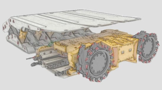
Figure 1. “Mikrus” longwall system [30].

The system is controlled by an operator using a central console located in the temporary storage gallery. The basic technical parameters of the system are shown in Table 1.

Table 1. Basic technical parameters of the system [30,31].

Parameter	Value
Cutting height	1100–1700 mm
Longwall length	260 m
Longitudinal longwall inclination	±35°
Transverse longwall inclination	±20°
Cutting head diameter	1200 ÷ 1600 mm
Working depth	600 mm
Supply voltage	3300 V
Overcut and undercut	50 mm
Minimum height of the cutting-loading head above the conveyor	850 mm
Minimum height in the working field	1000 mm
Maximum total installed power	633 kW
Maximum power of cutting head motor	500 kW
Maximum feed motor power	2 × 60 kW
Maximum winch motor power	13 kW
Maximum motor power of the conveyor drive	2 × 200/400 kW
Feed force (0–50 Hz)	2 × 320 kN
Feed rate	0–27 m/min
Longwall conveyor S-850N with the height of trough profile	220 mm
Conveyor scraper width	800 mm
Total weight of cutting and loading head	approx. 19.2 tons
Powered roof support Tagor-08,/16-POz	0.85 m–1.6 m
Assumed hourly capacity for 40 MPa coal strength	560 t/h
Assumed hourly capacity for 10 MPa coal strength	800 t/h

For more information on the “Mikrus” complex, see [30,31].

2.2. R Functions Used in Calculations

The R language was used to perform the calculations. It allows easy manipulation of large data sets by placing them in structures called data frames. The data prepared in this way are then processed using the functions of the R language. From the beginning of the development of this language, many libraries with functions covering a wide spectrum of calculations have been created. The significant fact is that it is an open-source language which allows researchers to add new features to its libraries as data science and analysis develop. Access to the libraries of the R system is provided by the CRAN archive. CRAN is a network of FTP and web servers around the world that store identical, up to date versions of code and documentation for R [32]. This language can run on the most popular operating systems, such as macOS, Windows, and most Linux distributions.

In addition to the standard functions built into the R language, the following libraries were used in the calculations: ggpolt2, dplyr, runner, and the replace_na_with_last function.

The ggplot2 library is a tool for creating advanced graphs. It allows for overlapping successive layers of graphs, assigning shapes and colors of objects depending on the value of attributes, automatic calculation and presentation of statistics, and creating panels and histograms [33]. The following functions were used in the presented research: ggplot, geom_line, geom_point, and geom_histogram.

Dplyr is a grammar of data manipulation, providing a consistent set of verbs that help one to solve the most common data manipulation challenges. [34]. From this package, the functions that were used in the calculations are: mutate, select, filter, arrange, and group_by.

Runner is a lightweight library for rolling windows operations. The package enables full control over the window length, window lag, and time indices [35]

In addition, the replace_na_with_last [36] function was used when restoring compressed variable values. In this function, a missing value of a variable can be filled with its last known value until the next known value appears.

3. Results and Discussion

The data used for the calculations were obtained when the shearer was tested under actual working conditions. They cover a period of two months and describe the values of the currents flowing through the windings of four shearer motors. One of the motors drives the cutting organs, two other motors are used to drive the shearer’s feed, and the fourth one drives the mechanism responsible for properly laying the power cables.

3.1. Data Preparation

The original data format contained 554,352 records with information about changes in current intensities, the time of their occurrence, and the code of the motor to which the change pertained, which appropriately reduced the amount of transmitted and collected data, but for its analysis, the original data layout had to be reconstructed.

R language functions were used to recreate the original data layout.

The processed dataset includes 5,254,993 records containing a timestamp, and four records containing the corresponding information about current. A fragment of the reconstructed set is shown in Table 2.

Table 2. Excerpt from the dataset.

tsu	ouf	npf	ngf	nuf
1364880939	31	32.3	32.4	16
1364880940	31	32.3	33.0	16
1364880941	31	33.6	33.6	16
1364880942	30	37.3	36.3	16
1364880943	32	41.6	39.5	16
1364880944	39	41.6	40.1	16
1364880945	48	41.6	39.1	16
1364880946	39	40.3	39.6	16

Source: Own study.

In Table 2, the column headings indicate, respectively:

• Tsu—time (unix timestamp);
• ouf—current of the shearing organ motor A;
• npf—current of the auxiliary drive motor A;
• ngf—current of the main drive motor A;
• nuf—current of the stacker motor A.

The data thus prepared were the basis for further calculations.

3.2. Preliminary Data Analysis—A Study of Current Intensity Distributions

Calculations were performed to determine histograms of current intensities for each motor. This allowed for revealing the nature of data variability. Calculation results are illustrated in Figure 2.

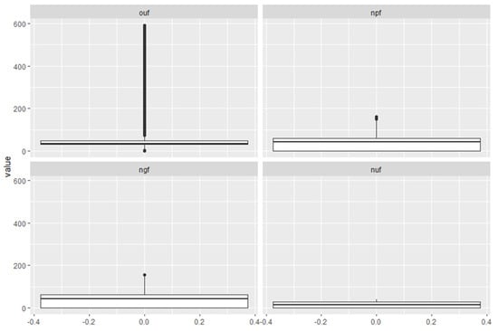
Figure 2. A box plot of the variability of the recorded parameters. Source: Own study.

As can be seen in Figure 2, a significant portion of the measured values of the cutting organ current (ouf) is at the lower end of the range of observed intensities, with outliers as high as 600 [A]. These are isolated situations associated with the starting of a particular motor. In order to better illustrate the variation of the remaining parameters, the values of current exceeding 200 [A] and equal to zero were eliminated from the graph, and another graph was then created (Figure 3).

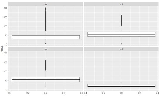
Figure 3. A box plot of the variability of the recorded parameters after rejecting extreme values. Source: Own study.

An analysis of the graph in Figure 3 reveals that the ranges of current intensities of the motors (ngf, npf) are very close to each other. The average value of these intensities is approximatly 42 A, and the interquartile range is ca. 24 A. The range of currents flowing through the motor of the cutting drive (ngf) is much larger and reaches up to 600 A (Figure 1), while the interquartile range is smaller than that of the drive motors and amounts to 17 A, and the mean of the observed values is ca. 35 A. As can be seen from the analysis of distributions, it should be noted that the terms ‘main engine’ and ‘auxiliary engine’ are conventional because the observed currents flowing through these engines are similar, and, moreover (as can be seen from other analyses), they operated simultaneously throughout the analyzed period.

3.3. Data Illustration

Using the ggplot function available in the R language, it is possible to generate graphs that can be customized in any possible way. A graph mapping the changes in currents as a function of time, recorded in the database, is presented below (Figure 4).

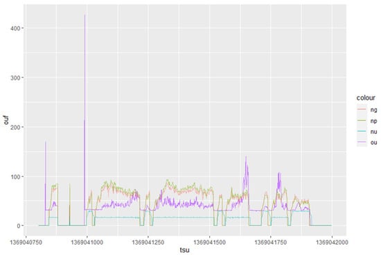
Figure 4. A plot of the variation of recorded current intensities as a function of time. Source: Own study.

In Figure 4, one can observe the periods of both work and standstill of the shearer. Purple is used for the values of current of the cutting unit motor (ou). In the presented period, there is a peak reaching the value exceeding 400 [A] connected with the starting of this motor. This is confirmed by the different increases in the currents flowing through the other motors. This figure illustrates the mutual similarity of the current values flowing through the two feed drive motors and the relatively constant current values flowing through the stacker drive motor.

3.4. Shearer Status Analysis

To investigate the nature of the load distribution of shearer motors in more detail, histograms of the values of the currents flowing through the main drive motor (Figure 5) and through the main feed drive motor (Figure 6) were generated.

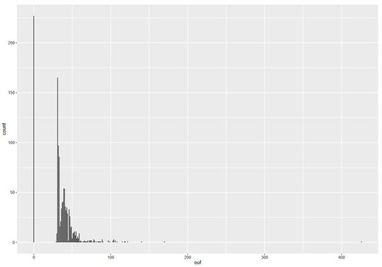
Figure 5. A histogram illustrating the current distribution of the cutting organ motor. Source: Own study.

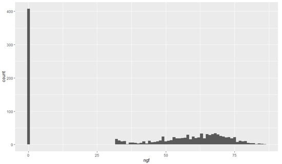
Figure 6. A histogram illustrating the current distribution of the main feed motor. Source: Own study.

Figure 5 presents a large number of observed zero values associated with device stoppage. In addition, there is a large number of observations of 30 [A] values which correspond to the movement of the cutting organ without the mining load. Higher values are observed during cutting.

In interpreting the distribution of current intensities in Figure 6, we can observe, similarly as before, a large number of zero value occurrences. However, in this case, it is difficult to clearly distinguish the values of current intensity corresponding to driving the shearer’s feed without the use of a cutting unit.

A better understanding of the operating state of the shearer can be obtained when the above histograms are overlayed. Figure 7 presents a graph resulting from superimposing the observations in the space formed by the currents of the cutter motor and the currents of the feed motor.

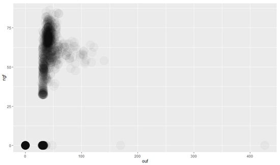
Figure 7. An illustration of the number of observations in the space of current intensities for two shearer motors. Source: Own study.

The number of observations corresponding to the values of these currents is mapped by the degree of blackness of a point in this coordinate system. This was accomplished by overlapping points with a high degree of transparency. In Figure 6, four operating states of the machine can be distinguished. The first one, in which the currents of both motors are zero, is the machine shutdown state. The second state is the idle state, which is a situation where the current of the feed motor is zero, while the current of the cutting unit motor is approximately 30 [A]. The third state is the maneuvering state. In this state, a current equal to approximately 30 [A] passes through both motors. It stands out in Figure 6 as a dark circle at the bottom of the point cloud. The last operating state of the shearer is the cutting state. In this state, the current of both the motor driving the cutting unit and the feed mechanism exceeds 30 [A].

Based on the boundaries assumed above, it is possible to assign the recorded readings of current intensity to the distinguished shearer working states and then to calculate the percentage structure of these states in the analyzed period of time. Taking economic calculations into account, the state of cutting is expected to occupy the largest part in this structure. The rules for assigning cutter operating states are summarized in Table 3.

Table 3. Assignment of operating states to observed current intensities.

ngf\ouf	0	0–33	>33
0	Off	Idle	X
>32	Maneuvering	Maneuvering	Extraction

Source: Own study.

The state marked with an “X” in Table 3 deserves an additional comment. It is a prohibited state. In this state, the shearer would mine coal without feed. Observations of this state are possible but only to analyze the incorrect operation of the shearer. An example would be to start the drive of the cutting organ that is hogged into a coal bed. This action can very likely result in damage to the machine.

The operation of the feed drive motors is analyzed in the next part of the study. Observations of the distributions of currents flowing through these motors and their waveforms observed on the graphs suggest a high similarity of these values. To confirm this, a graph was constructed (Figure 8) whose axes mark the currents of both motors.

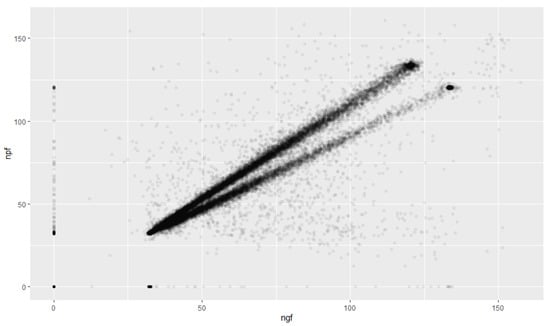
Figure 8. Mutual dependence of the loads on feed motors. Source: Own study.

In Figure 8, it can be seen that the points align along two distinct straight lines. The top line represents the cases where the power consumed by the main motor is greater than the power consumed by the auxiliary motor, while the bottom line represents the opposite case. It can also be seen that the difference between the currents flowing through the motors increases proportionally to their load. To better understand the structure of these cases, their percentages were calculated. The results are shown in Table 4. This list, as well as the rest of the analysis, does not include cases in which the feed drives were not working, because it concerns the states of a device in motion.

Table 4. Percentages of cases.

Case	Share (%)
main > auxiliary	52
main = auxiliary	1
main < auxiliary	47

Source: Own study.

Since the structure of these cases turned out to be uniform, a histogram was determined in the next step (Figure 9) which shows the distribution of differences between the currents of the two motors.

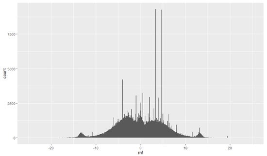
Figure 9. A histogram of differences in motor loads. Source: Own study.

The values to the right of zero are cases where the main motor draws more power than the auxiliary motor. This histogram is characterized by high symmetry, which, together with the percentage distribution calculated earlier, suggests that, to a significant extent, these motors swap roles in driving the shearer’s feed.

This observation is the basis for the hypothesis that shearer working directions can be distinguished. Since a significant longwall slope is likely to occur, there may be differences in loads between the motors driving the shearer feed. These differences may be increased by the activity of loading the excavated material onto a scraper conveyor, which is additionally performed by the moving shearer, and which may depend on the direction of the feed. Similar differences resulting from the direction of the shearer’s movement, but observed in the engines of the cutting units, were described in [37].

Partial confirmation of this hypothesis can be provided by the graph shown in Figure 10.

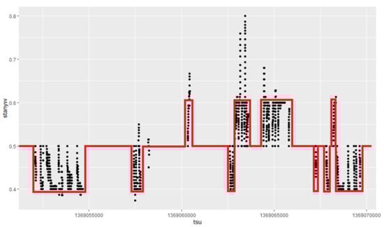
Figure 10. Changes in direction of shearer movement. Source: Own study.

Figure 10 was developed by introducing an additional variable (state) into the data set, based on the intervals determined in Figure 9. This variable takes values according to Table 5.

Table 5. Values of the ‘state’ variable in individual ranges of different currents of feed drive motors.

Interval	Value
(−∞, −12.5>	0.2
(−12.5, 2>	0.4
(−2, 2)	0.5
<2, 12.5)	0.6
<12.5, ∞)	0.8

Source: Own study.

To increase the clarity of the graph, the values of this variable were averaged within a fifteen-second window. The graph in Figure 10 covers a period of 5 h 30 min. The red line indicates the probable directions of the shearer’s movement (values of 0.4 and 0.6), and a value of 0.5 indicates its standstill.

3.5. Structure of Machine Operating States

Based on the rules determined in the analysis and collected in Table 3, a set of results (Table 6) was generated, showing the percentage structure of the machine operating states observed on consecutive days.

Table 6. Extract from the results of the machine structure.

Observation Day No.	Off	M	I	E
36	96.77	0.08	0.00	3.15
37	84.90	4.31	1.12	9.67
38	83.55	2.74	1.35	12.36
39	78.52	5.80	2.79	12.89
40	89.93	0.85	0.75	8.47
41	100	0	0	0
42	100	0	0	0

Source: Own study.

Table 6 presents the results of one week of observations. On all days, the vast majority of the time structure is occupied by the Off state. The largest share during the operation of the shearer is occupied by extraction activity (E) and the smallest share by the Idle (I) state. The maneuvering state is shown in column M. It should be recalled that the recorded data pertain to the period of implementation and testing of the shearer, and therefore, the results may significantly differ from those obtained in the conditions of industrial exploitation of the deposit.

4. Conclusions

The proposed method can serve as a verification tool for progress reported by employees. In a mine setting, the reporting of work through numbers provided by supervisory personnel is still used. The method described in this study enables a comparison of these values with the values calculated based on the analysis of current intensities, and thus, objective values can be obtained.

The results presented here do not include the shearer direction component, as the relationships discovered in the analysis must be further verified as a continuation of this work.

The presented analysis can also be an example of the fact that, in cases when the required process parameters are not available, they can be discovered based on other available parameters, which facilitates further analysis.

The authors believe that there is the need to develop a method to automatically separate groups of observations based on the shape of the histograms. Past considerations lead to determining the zero positions of the first derivative function approximating the quantitative distribution of observations.

The presented method can be implemented in information systems reporting the course of the production process in hard coal mines.

The calculations described in this paper are in line with the authors’ earlier works on monitoring the operation of machines. Issues related to identifying deviations from the norms of machine operation are presented in [38]. The subject of monitoring the analysis of the effectiveness of machine use in hard coal exploitation by generating reports enabling the analysis of the degree of machine use is presented in [39].

References

- Zhao, T.; Zhang, Z.; Tan, Y.; Shi, C.; Wei, P.; Li, Q. An innovative approach to thin coal seam mining of complex geological conditions by pressure regulation. Int. J. Rock Mech. Min. Sci. 2014, 71, 249–257. [Google Scholar] [CrossRef]
- Lorenz, U. Coal as fuel with good prospects/Węgiel jako paliwo z przyszłością. Przegląd Gór. 2005, 10, 8–14. (In Polish) [Google Scholar]
- Turek, M. Do not leave thin seams/Nie pozostawiajmy pokładów cienkich. Przegląd Gór. 2005, 10, 15–19. (In Polish) [Google Scholar]
- Zhang, L.M. The Current Situation and Developing Trend of Extremely Thin Coal Seam Mining of China. Appl. Mech. Mater. 2013, 295–298, 2918–2923. [Google Scholar] [CrossRef]
- Wang, J. Development and prospect on fully mechanized mining in Chinese coal mines. Int. J. Coal Sci. Technol. 2014, 1, 253–260. [Google Scholar] [CrossRef]
- Mamaikin, O.; Kicki, J.; Salli, S.; Horbatova, V. Coal industry in the context of Ukraine economic security. Min. Miner. Depos. 2017, 11, 17–22. [Google Scholar] [CrossRef]
- Griadushchiy, Y.; Korz, P.; Koval, O.; Bondarenko, V.; Dychkovskiy, R. Advanced experience and direction of mining of thin coal seams in Ukraine. In Technical, Technological and Economical Aspects of Thin-Seams Coal Mining, International Mining Forum; Taylor & Francis/Balkema: London, UK, 2007; pp. 1–7. [Google Scholar]
- Pavlenko, I.; Salli, V.; Bondarenko, V.; Dychkovskiy, R.; Piwniak, G. Limits to economic viability of extraction of thin coal seams in Ukraine. In Technical, Technological and Economical Aspects of Thin-Seams Coal Mining, International Mining Forum; Taylor & Francis/Balkema: London, UK, 2007; pp. 129–132. [Google Scholar]
- Korski, J.; Bednarz, R. Low shearer longwall system as an effective option to plough systems/ Kombajnowy system ścianowy jako efektywna alternatywa dla strugów ścianowych. Mech. Autom. Gór. 2012, 9, 31–38. (In Polish) [Google Scholar]
- Chai, W.Z. The lectotype of the thin coal bed synthesis mining equipment and the technological parameter optimizes. Sci. Technol. Tongmei 2007, 2, 2–4. [Google Scholar]
- Zhai, X.; Shao, Q.; Li, B.; Li, X. Shearer mining application to soft thin-seam with hard roof. Procedia Earth Planet. Sci. 2009, 1, 68–75. [Google Scholar] [CrossRef][Green Version]
- Wang, F.; Tu, S.; Bai, Q. Practice and prospects of fully mechanized mining technology for thin coal seams in China. J. S. Afr. Inst. Min. Metall. 2012, 112, 161–170. [Google Scholar]
- Lööw, J.; Abrahamsson, L.; Johansson, J. Mining 4.0—The Impact of New Technology from a Work Place Perspective. Min. Metall. Explor. 2019, 36, 701–707. Available online: https://link.springer.com/article/10.1007/s42461-019-00104-9 (accessed on 22 May 2021). [CrossRef]
- Bezerra, F.; Wainer, J. Anomaly detection algorithms in business process logs. In Proceedings of the Tenth International Conference on Enterprise Information Systems—Volume 2: ICEIS, INSTICC, Barcelona, Spain, 12–16 June 2008; SciTePress: Setúbal, Portugal; pp. 11–18. [Google Scholar] [CrossRef]
- Böhmer, K.; Rinderle-Ma, S. Automatic Signature Generation for Anomaly Detection in Business Process Instance Data. In Enterprise, Business-Process and Information Systems Modeling; Schmidt, R., Guédria, W., Bider, I., Guerreiro, S., Eds.; Springer International Publishing: Cham, Switzerland, 2016; pp. 196–211. [Google Scholar]
- Chen, D.; Panfilenko, D.V.; Khabbazi, M.R.; Sonntag, D. A model-based approach to qualified process automation for anomaly detection and treatment. In Proceedings of the 2016 IEEE 21st International Conference on Emerging Technologies and Factory Automation (ETFA), Berlin, Germany, 6–9 September 2016; pp. 1–8. [Google Scholar]
- Nolle, T.; Seeliger, A.; Mühlhäuser, M. Unsupervised Anomaly Detection in Noisy Business Process Event Logs Using Denoising Autoencoders; Discovery Science; Calders, T., Ceci, M., Malerba, D., Eds.; Springer International Publishing: Cham, Switzerland, 2016; pp. 442–456. [Google Scholar]
- Brzychczy, E.; Gackowiec, P.; Liebetrau, M. Data Analytic Approaches for Mining Process Improvement—Machinery Utilization Use Case. Resources 2020, 9, 17. [Google Scholar] [CrossRef]
- Zhou, J.; Li, X.; Mitri, H.S.; Wang, S.; Wei, W. Identification of large-scale goaf instability in undergroundmine using particle swarm optimization and support vector machine. Int. J. Min. Sci. Technol. 2013, 23, 701–707. [Google Scholar] [CrossRef]
- Hargrave, C.O.; James, C.A.; Ralston, J.C. Infrastructure-based localisation of automated coal mining equipment. Int. J. Coal Sci. Technol. 2017, 4, 252–261. [Google Scholar] [CrossRef]
- Jedliński, Ł.; Gajewski, J. Optimal selection of signal features in the diagnostics of mining head tools condition. Tunn. Undergr. Space Technol. 2019, 84, 451–460. [Google Scholar] [CrossRef]
- Bodlak, M.; Kudełko, J.; Zibrow, A. Machine Learning in predicting the extent of gas and rock outburst. E3S Web Conf. 2018, 71. [Google Scholar] [CrossRef]
- Verma, A.K.; Kishore, K.; Chatterjee, S. Prediction Model of Longwall Powered Support Capacity Using Field Monitored Data of a Longwall Panel and Uncertainty-Based Neural Network. Geotech. Geol. Eng. 2016, 34, 2033–2052. [Google Scholar] [CrossRef]
- Deb, D.; Kumar, A.; Rosha, R.P.S. Forecasting shield pressures at a longwall face using artificial neural networks. Geotech. Geol. Eng. 2006, 24, 1021–1037. [Google Scholar] [CrossRef]
- Mahdevari, S.; Shahriar, K.; Sharifzadeh, M.; Tannant, D.D. Stability prediction of gate roadways in longwall mining using artificial neural networks. Neural Comput. Appl. 2017, 28, 3537–3555. [Google Scholar] [CrossRef]
- Kopacz, M. The impact assessment of quality parameters of coal and waste rock on the value of mining investment projects—Hard coal deposits. Miner. Resour. Manag. 2015, 31, 161–188. [Google Scholar] [CrossRef][Green Version]
- Jonek-Kowalska, I.; Turek, M. Dependence of total production costs on production and infrastructure parameters in the polish hard coal mining industry. Energies 2017, 10, 1480. [Google Scholar] [CrossRef]
- Qiao, W.; Liu, Q.; Li, X.; Luo, X.; Wan, Y.L. Using data mining techniques to analyze the influencing factor ofunsafe behaviors in Chinese underground coal mines. Resour. Policy 2018, 59, 210–216. [Google Scholar] [CrossRef]
- He, Z.; Wu, Q.; Wen, L.; Fu, G. A process mining approach to improve emergency rescue processes of fatal gas explosion accidents in Chinese coal mines. Saf. Sci. 2019, 111, 154–166. [Google Scholar] [CrossRef]
- FAMUR. Available online: https://famur.com/kompleks-mikrus-1 (accessed on 22 May 2021).
- Dziura, J. Mikrus Complex—A new technology of extraction low decks/Kompleks Mikrus—Nowa technologia wybierania pokładów niskich. Masz. Gór. 2012, 3, 3–11. (In Polish) [Google Scholar]
- The Comprehensive R Archive Network. Available online: https://cran.r-project.org/ (accessed on 22 May 2021).
- GGPLOT2. Available online: https://ggplot2.tidyverse.org/ (accessed on 22 May 2021).
- DPLYR. Available online: https://dplyr.tidyverse.org/ (accessed on 22 May 2021).
- Package “Runner”. Running Operations for Vectors. Available online: https://cran.r-project.org/web/packages/runner/runner.pdf (accessed on 22 May 2021).
- Replacing NAs with Latest Non-NA Value. Available online: https://stackoverflow.com/questions/7735647/replacing-nas-with-latest-non-na-value (accessed on 22 May 2021).
- Jaszczuk, M. The influence of the load condition shearer on the possibility of obtaining a high concentration of mining Wpływ stanu obciążenia kombajnu ścianowego na możliwość uzyskania wysokiej koncentracji wydobycia, Gliwice. Zesz. Nauk. Politech. Śląskiej 1999, 240, 19–25. (In Polish) [Google Scholar]
- Kęsek, M. Analysing data with the R programming language to control machine operation/ Analiza danych z wykorzystaniem języka R w kontroli pracy maszyn. Inżynieria Miner. 2019, 1, 231–235. [Google Scholar] [CrossRef]
- Kęsek, M.; Ogrodnik, R. Computer aided monitoring and analysis of machine work/Komputerowe monitorowanie i analiza pracy maszyn. Mark. Rynek 2018, 9, 383–395. (In Polish) [Google Scholar]
Publisher’s Note: MDPI stays neutral with regard to jurisdictional claims in published maps and institutional affiliations. |
© 2021 by the authors. Licensee MDPI, Basel, Switzerland. This article is an open access article distributed under the terms and conditions of the Creative Commons Attribution (CC BY) license (https://creativecommons.org/licenses/by/4.0/).