Abstract
Wind and solar energies present a time and space disparity that generally leads to a mismatch between the demand and the supply. To harvest their maximum potentials, one of the main challenges is the storage and transport of these energies. This challenge can be tackled by electrofuels, such as hydrogen, methane, and methanol. They offer three main advantages: compatibility with existing distribution networks or technologies of conversion, economical storage solution for high capacity, and ability to couple sectors (i.e., electricity to transport, to heat, or to industry). However, the level of contribution of electric-energy carriers is unknown. To assess their role in the future, we used whole-energy system modelling (EnergyScope Typical Days) to study the case of Belgium in 2050. This model is multi-energy and multi-sector. It optimises the design of the overall system to minimise its costs and emissions. Such a model relies on many parameters (e.g., price of natural gas, efficiency of heat pump) to represent as closely as possible the future energy system. However, these parameters can be highly uncertain, especially for long-term planning. Consequently, this work uses the polynomial chaos expansion method to integrate a global sensitivity analysis in order to highlight the influence of the parameters on the total cost of the system. The outcome of this analysis points out that, compared to the deterministic cost-optimum situation, the system cost, accounting for uncertainties, becomes higher (+17%) and twice more uncertain at carbon neutrality and that electrofuels are a major contribution to the uncertainty (up to 53% in the variation of the costs) due to their importance in the energy system and their high uncertainties, their higher price, and uncertainty.
1. Introduction
To ensure the energy supply of a more and more demanding society in a context of environmental crisis, major transformations are needed. Besides behavioural changes, an overall reshape of the energy system is necessary in terms of both primary energy sources and technologies used to convert these resources into the end-use demand (EUD) (i.e., the energy service required by the the final consumer) [1]. In this perspective, variable renewable energy sources (VRES) such as wind and solar, have already emerged as the keystone to defossilise the energy system. However, their intermittency and space disparity could hold back their vaster integration in the future. To address this issue, due to some limitations (e.g., range, power, costs) of electricity-focused solutions such as direct current (DC) lines, the transport and long-term storage of the renewable electricity produced in excess should be optimised.
This challenge can be tackled by electrofuels [2]. These fuels represent energy carriers where electricity has the major share in the energy balance of the fuel [3]. In practice, this electricity is mainly converted into hydrogen (i.e., electrolysis) and then potentially upgraded into more complex fuels (e.g., methane, methanol, or ammonia). Even if the share of electricity increases in the energy system through the electrification of the end-use demand, gaseous and liquid fuels will keep on being big players during (and after) the energy transition [4]. They offer three main advantages: infrastructure compatibility, storage, and capacity to link sectors (i.e., from electricity to mobility, heat, or industry). Development on electrofuels aims at making them more and more compatible with existing and mature technologies [4]. An example is carbon-free ammonia–hydrogen blends burned in spark ignition engines [5] or combined heat and power (CHP) applications [6]. With a growing share of VRES, sector coupling is essential to absorb the surplus of electricity from these intermittent production means [7] and integrate them more cost-effectively [8,9]. Besides direct electrification of other sectors (e.g., electrical heat pumps, battery electric vehicles), Brown et al. [10] showed that converting power to hydrogen and methane was advantageous at high shares of renewables, in their optimisation of the European whole-energy system. Electrofuels have the ability to couple energy and non-energy sectors [11]. For instance, electricity produced in excess from VRES can be converted in ammonia through the Haber–Bosch process and subsequently transformed into fertiliser—coupling the power and industry sectors [12]. Gas networks present much more storage potential than electrical networks (e.g., 50 times more in Germany and 300 times more in France) [13]. Where batteries exhibit limited storage capacity (up to 10 MWh) as well as self-discharge losses, electrofuels are an economical solution for high capacity (from 100 GWh) and long-term (i.e., from months to years) storage of energy [14,15]. Besides storing energy, in their analysis of the German transport sector in 2050, Millinger et al. [16] highlighted that producing electrofuels can represent a better usage of the ambient CO2 than carbon capture and storage (CCS) to supply hydrocarbon fuels while limiting the curtailment of VRES. Moreover, some applications (e.g., marine, aviation, and heavy-duty transport) will be hard to electrify and keep on requiring high-density energy carriers [17,18]. These carriers, currently produced mostly from fossil resources, will still consist of hydrocarbons in a renewable world. This is why this paper uses “defossilisation” rather than “decarbonisation” as carbon will still play a key role in a carbon neutral energy transition [19].
To harvest the maximum potential of synthetic energy carriers in a sustainable transition and maximise the overall system efficiency [20], it is necessary to study the integration of these fuels within a multi-sector and whole-energy system [21]. To reach this goal, an energy system optimisation model (ESOM) can define the design of the system to minimise, for instance, its costs or its emissions [22]. In this research field, Yue et al. [23] highlighted that most of ESOMs use a deterministic approach (i.e., 75% out of the 134 reviewed ESOM studies). However, the model structures are inherently uncertain as well as their numerous composing parameters, especially when it comes to define an energy transition strategy for a large-scale system, such as a country. Given the lifetime of the conversion technologies, such strategy implies decisions with long-term impacts (20 to 50 years) where forecasts can be highly unreliable [24]. Besides the uncertainty on the model structure (not addressed in this work), this long-term and large-system optimisation motivates the need to account for uncertainty quantification (UQ) and consider it as a major challenge of such models [25]. This challenge, along with a large number (i.e., more than a hundred) of uncertain parameters and limited information of their distribution, leads to the “curse of dimensionality” [26].
To assess the importance of the electrofuels in a defossilised energy system, this work gives the results of an uncertainty quantification performed on a whole-energy model, EnergyScope Typical Days (EnergyScope TD) [27]. It optimises the investment and operation strategies to meet the end-use demand of the system (i.e., electricity, heat, and mobility) and minimise its total annual cost [28]. Based on previous research on the Belgian energy system [29] and uncertainty characterisation [24], this analysis applies the polynomial chaos expansion (PCE) method [30]. PCE provides a computationally efficient alternative to the Monte Carlo simulation for uncertainty quantification to address the “curse of dimensionality” [31]. Given limited information about the uncertainty of the parameters for long-term energy planning models [28], PCE builds a surrogate model in a computationally efficient way [32]. Based on this surrogate model, this paper highlights the most-impacting parameters through their sensitivity indices (i.e., Sobol’ indices) and extracts valuable statistical moments (e.g., mean- or variance-) of the total cost of the system. PCE has been applied in various energy system evaluations to quantify the statistical performance [33]. Limpens et al. [34] showed the relevance of using the PCE method by comparing it with the Morris method [35] used in similar studies [24,36]. Coppitters et al. [37] constructed a PCE on a photovoltaic-electrolyser system design and, based on the Sobol’ indices, bulk manufacturing of the electrolyser and more demonstration projects are suggested to reduce the variance on the levelised cost of hydrogen. Similarly, Verleysen et al. [12] quantified the Sobol’ indices from a PCE on a power-to-ammonia system and highlighted that an accurate flow meter and improving the temperature control in an ammonia reactor are the main actions to render the performance more robust.
The novelty of this paper consists in the combination of applying the PCE to a whole-energy system and studying the impact of electrofuels in this global sensitivity analysis (GSA). This paper aims at (i) illustrating the impact of considering uncertainties (compared to deterministic analysis) for long-term energy planning models; (ii) identifying the parameters critical to the uncertainty of the total cost of a whole-energy system; (iii) highlighting the role of electrofuels in regard to the objective of decreasing the greenhouse gas (GHG) emissions—the ”climate targets”. Thanks to these analyses, the present work could help providing to policy makers with insightful guidelines to answer the following questions: to what extent uncertainties should be taken into account when planning low-carbon energy system? Given the limited availability of local renewables in Belgium, what solutions of the Mix scenario presented by Limpens et al. [29] (e.g., electrification, nuclear energy, import of renewable molecules) would affect the most the variation of the total cost of the system?
The paper is structured as follows: Section 2 details the considered electrofuels, the whole-energy model (EnergyScope TD), the reference case study, the Belgian energy system in 2050, and the approach to analyse different climate targets. Then, Section 3 presents the methodology to characterise the uncertainties, to carry out the global sensitivity analysis via the PCE. Finally, Section 4 depicts the evolution of the statistical moments of the costs, the critical parameters, and the role of electrofuels for different climate targets. Section 5 analyses these results and puts them into a broader perspective to conclude with future research directions in Section 6.
2. Model of the Whole-Energy System and Its Defossilisation
Through this section, the considered electrofuels are described as well as the open-source model, the reference case study and the approach to analyse its defossilisation.
2.1. Electrofuels
To cover a wide range of applications and conversion technologies, this work considers three families of electrofuels: hydrogen, electro-methane and electro-liquid fuels. The first one is the cornerstone of the energy transition [38], as the first molecule to be converted from electricity through electrolysis as well as the fundamental chemical building block for more energy-dense fuels. In its sustainable development scenario (SDS), IEA [39] expects about hundred times more hydrogen to be consumed (from 0.45 Mt to 40 Mt, worldwide) between 2020 and 2030. The two other fuels aim at substituting their fossil equivalents, respectively natural gas and liquid fossil fuels (e.g., gasoline, diesel, and light fuel oil). Technologies are implemented in the model to produce these fuels locally (e.g., electrolysis to produce hydrogen and, subsequently, from hydrogen, further processes can produce electro-methane or electro-liquid fuels with an added renewable C-source) or import them. When imported from abroad, these electrofuels are assumed to be produced from renewable electricity. Therefore, this work allocates them a zero-global warming potential (GWP) (i.e., kt/GWh). In practice, there is always a residual CO2-impact that has to be compensated for (i.e., through biomass or direct air capture) [40]. However, the study of these actual CO2-compensation means is out of the scope of this work. Finally, this paper considers a nominal cost of import () of 160 €/MWh, 180 €/MWh, and 190 €/MWh, respectively, for hydrogen, electro-methane, and electro-liquid fuels. These costs are taken as the average production costs of the respective fuels from a previous work on electrofuels for the transport sector [18]. In the aforementioned work, based on an extensive literature review, the authors split the production cost of each fuel over the different production steps (i.e., water electrolysis, carbon capture, and fuel synthesis) considering different technologies for each step. After a scenario and sensitivity analysis of parameters affecting the electrofuels production cost (e.g., investment and operation cost of the electrolyser, price of electricity, cost of CO2 capture), these authors suggested a range of production costs for a whole set of electrofuels (i.e., methane, methanol, dimethyl ether (DME), gasoline, and diesel). From this range, the present work extrapolated nominal values for the production cost of the fuels in 2050. Even if these costs do not reflect the market prices, this implementation accounts for the future evolution forecast of the price. This is consequently consistent with the implementation of the other imported resources. Regarding their uncertainty, this work assumes the same range of variation on these nominal costs as the one applied to the price of imported fossil fuels (e.g., natural gas, light fuel oil, and diesel) from [24]: . Through their uncertainty characterisation, Moret et al. [24] applied in parallel five criteria to each uncertain parameter of their model. Amongst these criteria, ranges already proposed in the literature and existing forecasts allow the authors to suggest the aforementioned range for this uncertainty considered as aleatory (i.e., future, irreducible uncertainty) and constant over time.
2.2. Model of the Energy System
The model used in this study is EnergyScope TD [27]: a linear programming (LP) open source model for the regional whole-energy (i.e., multi-sector and multi-carrier) system, such as a country, that has been validated for the case study of interest, i.e., the Belgian whole-energy system, by Limpens et al. [29]. This model uses a bottom-up approach in the sense that it focuses on a set of individual technologies to deliver specific energy demands (i.e., electricity, heat, and mobility) in a way that optimises the costs and benefits associated with investments and operation within the system [41]. In terms of spatial resolution, the country is modelled as a single node where transmissions within the country are not considered. Similar to the copper plate model of a power grid, it is assumed that the demands have to be supplied by the production, regardless of the flows between the producers and the consumers. Yet, adapting the networks are accounted for in terms of the required investments. For instance, a high share of VRES requires an investment to reinforce the power grid (i.e., around 350 M€/GW of installed capacity of VRES) [42]. In EnergyScope TD, the demands are impose in terms of an EUD instead of a final energy consumption (FEC). For instance, the passenger mobility is defined in passenger kilometers per year rather than in a certain amount of gasoline to fuel cars or electricity to power trains. The data for the transport demand come from the European Commission [43]. They account for all the transportation except the one outside Europe as they stipulate: “(3) Excluding international extra-EU aviation.”. In other words, it accounts for the local (i.e., endogenous) mobility for freight and passengers plus the international trips within Europe. However, it does not account for the international transportation outside Europe, which represents the long-range flights and most of the maritime freight. Given the exogenous EUD in electricity, heat, and mobility over a target future year (snapshot approach [44]), the availability, and the cost of the resources () (e.g., natural gas (NG), wind and solar energies, biomass) and the efficiency and the cost of the endogenous conversion technologies () (e.g., power plants, wind turbine, heat pumps, cars), the model optimises the investment and the operation strategies to minimise the total annual cost of the system ():
where and account for the annualised investment cost of a technology (Equation (2)) and its operation and maintenance costs (Equation (3)), respectively, whereas is the operating cost of a resource (Equation (4)):
where and are the specific investment and maintenance costs of a technology, respectively, while is its installed capacity. In Equation (4), is the specific cost of the resource, is the period duration, and is the actual use of the resource in each period. As detailed in [27], “h” and “td” stand for the hour of the typical day and the typical day, respectively. Moreover, summing over the different typical days (TDs) and over the hours of TDs, using the set , is equivalent to summing over the 8760 h of the year.
A technology lifetime () and the interest rate () allow us to compute the annualising factor, :
Among other constraints, we define the climate targets by putting a limit, , on the total yearly emissions of the system () related to the resource emissions ():
where is the specific emissions of each resource. These GHG emissions are calculated using a life cycle assessment (LCA) approach and following the indicator “GWP100a-IPCC2013” developed by the Intergovernmental Panel on Climate Change (IPCC) [45]. For the resources, these GHG emissions account for extraction and transportation, on one hand, and combustion, on the other hand. For instance, the 267 kg accounted for the natural gas are split between 67 kg for the former and 200 kg for the latter [46]. Similarly to official agencies (i.e., European Union Commission or International Energy Agency) and previous works [27,29], this analysis considers this metric as the “climate impact” of the whole-energy system. The part of CO2 related to the combustion is therefore considered explicitly in the model, similar to any other commodity, that can be produced (e.g., to produce 1 GWh of electricity, a natural gas combined cycle (CCGT) burns 1.55 GWh of NG and emits 0.32 kt) and consumed (e.g., besides 1.45 GWh of hydrogen, the methanolation process consumes 0.25 kt to produce 1 GWh of “synthetic liquid fuel”).
Finally, EnergyScope TD has an hourly resolution ( is equal to one hour) and a tractable formulation (1–5 min computational time). The former allows for a fine analysis of a high integration of VRES and storage capacities. The latter, necessary to keep the uncertainty quantification (i.e., 1980 runs) computationally affordable, is due to the use of typical days, 12 in the case of this work. Compared to a reference case where each of the 8760 h of the year were simulated, Limpens et al. [27] showed that opting for 12 typical days was a good trade-off between limited impact on the resulting energy system strategy (i.e., the installed capacity of the technologies and the use of resources remain in the same order of magnitude) and a significant gain in computational time (i.e., from 70,240 s for the reference case to 91 s for the 12-TD case). Figure 1 gives an overview of the model operation and the way the GSA was performed.
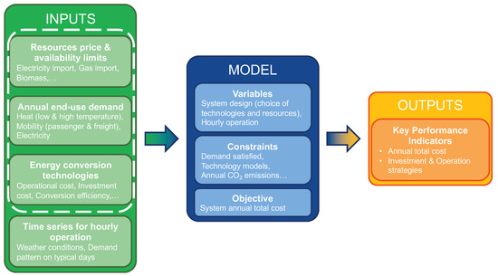
Figure 1.
Schematic of the EnergyScope TD model [34]. Dash-boxed inputs point out the uncertain parameters (, , …, ) that will be analysed during the GSA on the total annual cost of the system.
2.3. Reference Case Study: The Belgian Energy System in 2050
The case study is the Belgian energy system in 2050, as the long-term objective for carbon neutrality. Limpens [42] summarised the data used in this study, the documentation of the model, and its code repository.
The energy system has to supply eight exogenously imposed demands split into three main categories: electricity, heat, and mobility. To meet these three categories of demands, EnergyScope TD integrates twenty different resources either from import (e.g., electricity, electrofuels, biofuels, NG, gasoline, uranium) or locally available (e.g., solar, wind, geothermal, woody and wet biomass). Similarly to Limpens [42], to limit the Belgian electrical dependence on neighbouring countries, the yearly imports of electricity are limited to 30% of the yearly electricity end-use demand (i.e., 32.43 TWh maximum of imported electricity). Like Limpens et al. [29], this study accounts for a limited area available for solar photovoltaic (PV), i.e., up to 250 km, in accordance with Devogelear et al. [47]. As detailed by Limpens et al. [29], to convert these resources into the different demands, the model counts many technologies to produce different energy carriers: electricity (9 technologies), heat (31 technologies among which CHP plants that also produce electricity), and freight and passenger mobility (20 technologies). In accordance with previous research [48], additional constraints drive the mobility sector to represent it more realistically. On one hand, given the major role played by private cars in the Belgian passenger mobility (i.e., around 80% [48]), public transport (e.g., tramways, buses and trains) can only supply half of it. On the other hand, trains and boats can provide up to 25% and 30% of the freight mobility, respectively, while the rest is supplied by road transport, i.e., trucks. Additionally, the model accounts for different infrastructures (21 technologies). The latter encompasses, for instance, the power grid, the district heating networks (DHN), the mobility infrastructures (e.g., roads, railways) as well as technologies to produce “synthetic fuels” (e.g., wood pyrolysis, biomethanolation, or steam methane reforming (SMR) to produce hydrogen). In addition to these conversion technologies, the model includes 21 technologies to store electricity, heat, and fuels.
Current Belgian energy policies plan on phasing out local production of nuclear electricity. However, in Belgium, reaching the goal of energy transition will not be a “winner-takes-all” situation but rather a combination of technologies, implemented simultaneously [29]. This mix of solutions allows us to reach more ambitious reduction of CO2 emissions. As we aim at performing a GSA of a low-CO2 Belgian energy system, we implemented a similar “mix” scenario. In addition to the most realistic scenario presented by Limpens et al. [29] (i.e., harnessing full potential of local renewables and allowing import of electricity and renewable fuels), this study allows using up to the current 5.62 GW nuclear power plants capacity and non-proven endogenous renewable resources such as additional offshore wind and geothermal (i.e., up to 2 GW thermal and 2 GW electric) capacities. Regarding the nuclear capacity and the geothermal potential, the deterministic case presented in Figure 2 considers their average value between 0 and maximum capacity: 2.81 GW of nuclear power plants and 1 GW and 1 GW of geothermal. Without fixing , EnergyScope TD reaches a cost-optimum Belgian energy system in 2050 at around 43 b€/year and 72 MtCO2. Comparatively, the actual Belgian energy system in 2015 emitted 127 MtCO2 (considering the same “GWP-accounting” as described in Section 2.2) and had an estimated total cost of 43.6 b€/year according to Limpens [42], for the demands summarised in Table 1. As detailed by Limpens et al. [29], in 2015, the Belgian energy system was dominated by fossil fuels (70% of the 620 TWh primary energy mix) to supply these demands. Besides these, nuclear energy, electricity import, and waste account for 19%, 3%, and 1%, respectively, where renewables (i.e., 15 TWh of woody biomass, 6 TWh of wind, and 3 TWh of solar) complete the mix. Appendix A provides more details about the major technologies to supply the demands.

Figure 2.
Energy flows in the reference scenario representing the Belgian energy system in 2050, without climate target and with nominal values of the parameters. The left-hand side gathers all the resources and the right-hand side gathers the final energy consumption. In between, the conversion technologies. Abbreviations: natural gas (NG), combined heat and power (CHP), curtailment (Curt.), district heating networks (DHN), di-hydrogen (H2), heat pump (HP), high temperature (HT), low temperature (LT), storage (sto), decentralised (Dec), private and public mobility (Mob priv and Mob public), and exports and losses (Exp & Loss).

Table 1.
Comparison of EUD for the years 2015 (actual) [42] and 2050 (forecast) [49]. Abbreviations: temperature (Temp.), passenger (pass.), and tons (t).
Figure 2 shows the entire conversion chain between the resources and the final energy consumed for the reference case study, without limiting the GHG emissions (and with parameters at nominal values). This case is called “reference scenario-100%”. Even if EnergyScope TD optimises the system to meet the end-use demand (EUD), we decided to represent the final energy consumed on the Sankey diagram of Figure 2 to be able to compare the mobility sector (of which EUD is expressed in passenger-kilometer (pkm) and ton-kilometer (tkm)) with the other energy sectors. As shown by Limpens et al. [29], this scenario represents an ecological and economical interest compared to the actual energy system of today, by relying on more efficient technologies and harnessing more of the renewable potential. The primary energy mix (420 TWh) is dominated by non-renewable sources (70%): natural gas, uranium, and coal account for 208.0 TWh, 52.1 TWh, and 33.4 TWh, respectively. Renewables stand for 26% of the primary energy supply split between wet biomass (38.9 TWh), wind (31.9 TWh), solar (20.8 TWh), geothermal (15.8 TWh), and hydro (0.5 TWh). The remaining 4% consist of local non-renewable wastes (17.8 TWh) and imported electricity (0.5 TWh). The electricity generation is equally shared between renewable and non-renewable sources. The passenger mobility relies on fuel cell cars, tramways, and NG buses while fuel cell trucks, trains, and NG boat provide the transport of freight. Besides the geothermal used at its full potential for DHN, low-temperature heat demand is fully supplied by heat pumps. Waste and wood boilers are the biggest players to supply the industrial high-temperature heat demand, besides a small share coming from natural gas CHP. Finally, we observe that electrofuels are too expensive to compete against their fossil equivalents when there is no constraint on the CO2 emissions.
It is important to remind that such a system is the result of a linear optimisation. This means that a small difference (e.g., efficiency, cost of investment) can make the system switch between two different solutions but with a similar cost objective. This is another rationale to account for uncertainties in such a research field.
2.4. Description of the Defossilisation
As illustrated in Figure 3, from the cost-optimum of the Belgian energy system in 2050 presented in Section 2.3, this analysis forced the total annual emissions of the system to decrease by reducing its upper limit (i.e., in Equation (6)).
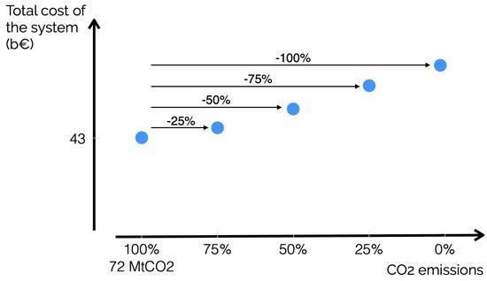
Figure 3.
Method to force the system to phase out fossil fuels. While keeping a cost-optimisation of the system, the is gradually decreased. This strategy gives the following points of analysis: 100% (i.e., no limitation on the total GWP), 75%, 50%, 25%, down to 0%. To reach carbon neutrality, the assumption is made that uranium, local waste, and wet and lignocellulosic biomass have a 0-GWP. In addition, in this “0%-scenario”, there is no more import of electricity as there is an uncertainty on its GWP impact, ∈ [0; 0.1] kt/GWh.
In practice, 25% steps of GWP reduction were made from the “reference scenario-100%” detailed in Section 2.3. This strategy gives the following points of analysis: 100% (i.e., no limitation on the total GWP), 75%, 50%, 25%, and down to 0%. As the goal of the work is to study major trends of energy system strategies facing different GWP constraints, it is important to note that these strategies result from distinct snapshot optimisations assuming green field for every technology, without pathway to link them with each other. To represent the carbon neutrality scenario, the simplifying assumption is made that uranium, local waste, and wet and lignocellulosic biomass have a 0-GWP, similar to the electrofuels presented in Section 2.1. In addition, in the “0%-scenario”, there is no more import of electricity as there is an uncertainty on its GWP impact, = [0; 0.1] kt/GWh. Then, for each of these climate targets (including the “100%” case) for the same target year (i.e., 2050), PCE is applied to highlight the critical parameters (thanks to Sobol’ indices, see Section 3.2) and extract statistical moments of the total annual cost of the system. In the rest of this work, a higher climate target has to be understood as a bigger CO2-emissions reduction and, consequently, a smaller value for .
3. Uncertainty Quantification
In this section, the uncertainty characterisation is briefly presented. It will serve in the global sensitivity analysis carried out through the PCE method on the selected uncertain parameters.
3.1. Uncertainty Characterisation
Accounting for uncertainties in energy system long-term planning is crucial [50] and challenging given inaccurate forecasts and scarcity of data [24,28]. To address this challenge, Moret et al. [24] developed a methodology to define ranges of parameter uncertainties. These ranges were originally defined for the Swiss energy system and have been adapted for the additional technologies to fit with the case of Belgium. Table 2 gives the uncertainty ranges applied for some key parameters. Like Li et al. [51], this work assumed that all the uncertain parameters are independent and uniformly distributed between their respective lower and upper bounds. The exhaustive list of the uncertainties of these parameters is given in Appendix B.
Table 2.
Illustration of the uncertainty characterisation for different parameters. Abbreviation: natural gas (NG).
3.2. Polynomial Chaos Expansion
The uncertainty on the model input parameters propagates through the model, resulting in uncertain performance indicators. Due to the computational cost of the system model (90 s), we chose polynomial chaos expansion (PCE) to quantify the uncertainties [37]. A PCE surrogate model of the system model consists of a series of multivariate orthonormal polynomials with corresponding coefficients [30]:
where is a random vector with the independent components and represents the multi-indices stored in the set . The size of , which equals the number of coefficients in the PCE, is defined by a truncation scheme. In this work, a typical truncation scheme is assumed, which limits the multivariate polynomial order in the expansion up to a certain degree. Hence, the number of multi-indices in the set equal to
where p corresponds to the polynomial order and is the stochastic dimension, i.e., the number of random variables [30]. Consequently, the PCE consists of coefficients. To quantify these coefficients, least-square minimisation is applied [52]. To ensure a well-posed least-square minimisation, samples are generated () and evaluated in the system model. The results are stored in a vector . Thereafter, an information matrix is quantified, based on the basis polynomial evaluations onto each sample:
The coefficients follow out of the least-square minimisation solution:
Out of the PCE coefficients, the mean, , and standard deviation, , of the quantity of interest (i.e., the total cost of the energy system) follow analytically:
In addition to these statistical moments, the Sobol’ indices can be deduced from the coefficients as well. The total-order Sobol’ indices illustrate the contribution of each stochastic input parameter to the variance of the quantity of interest, including the mutual interactions. The total-order Sobol’ index for a stochastic parameter i is quantified as follows:
3.3. Preliminary Screening and Selection
Similarly to previous studies [24,34], parameters of the model have been first screened to group them into 120 sets. For instance, the uncertain price of imported fossil hydrocarbons impact, similarly, the price of imported coal, natural gas, light fuel oil, gasoline, and diesel. As performing an accurate GSA on so many parameters would require almost 600,000 runs and, consequently, would not be affordable (i.e., the “curse of dimensionality”), a pre-selection was required. This pre-selection has been carried out after five (i.e., to ensure redundancy) first-order PCE on the 120 sets. In this process, only 43 uncertain parameters were kept, based on good practice [53], where parameters with a Sobol’ index above the threshold (where is the number of uncertain parameters at the pre-selection phase) are called critical parameters and considered for the rest of the study. Finally, to limit the error (i.e., below 1% as proposed by Coppitters et al. [52]) on the statistical moments, one second-order PCE was performed on the remaining 43 uncertain parameters (i.e., and in Equation (9)).
4. Results
This section shows the results of the GSA performed on the Belgian energy system in 2050 subject to different climate targets. First, the total annual cost of the system is analysed through its statistical moments and its probability density function (PDF). Second, the most critical parameters are listed according to their respective Sobol’ indices.
4.1. Statistical Analysis of the Cost
As detailed in Section 3.2, the PCE coefficients allow to extract statistical moments (e.g., mean and variance) of the total annual cost, without additional computational cost. On top of it, we can construct the PDF of this output of interest by a Monte Carlo approach with the obtained surrogate model, which takes negligible (i.e., few seconds) computational time. Figure 4 shows this PDF of the total annual cost, at each climate target, and the evolution of the 95% () confidence interval. Table 3 gives the mean, the standard deviation of the total annual cost, and the ratio between these two metrics.
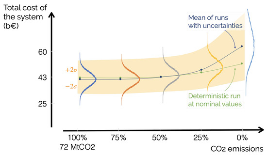
Figure 4.
PDF of the total annual cost of the energy system at each climate target and the 95% confidence interval. The trend lines give the mean of the runs performed during the GSA (blue curve) and the result of the deterministic runs at the nominal value of the parameter (green curve).
Table 3.
Mean, standard deviation of the total annual cost, and ratio between these two metrics, the coefficient of variation (CoV).
First, phasing out cheap fossil fuels and relying more and more on renewables and import of electrofuels naturally drives up the cost of the system. Then, the different PDFs show that defossilising the energy system makes it more uncertain as the interval widens, even “faster” than the increase in the mean, as shown in Table 3. Finally, given the trend lines, we understand how important it is to take into account the uncertainties in long-term energy planning. Indeed, the uncertainty characterisation presented in Section 3.1 leading to some off-centre range of uncertainties, which makes the deterministic optimisation underestimate the cost, especially at higher climate targets (e.g., by 15% on average for the “0%” case).
4.2. Critical Parameters
Figure 5 illustrates the evolution of the Sobol’ index of the Top-5 parameters along the defossilisation. As explained in Section 3.2, this shows the contribution to the variance of the total annual cost of the system. Most of the key parameters are cost-related: (i) price of fossil hydrocarbons that affects the cost of imported coal, natural gas, light fuel oil, gasoline, and diesel (), (ii) investment cost of fuel cell for transport vehicles using this propulsion technology (), (iii) investment cost of cars (), and (iv) the price of imported electrofuels as listed in Section 2.1 (). The last impacting parameter is (v) the maximum capacity of nuclear power plants (). Table 4 gives the range of variation for each of these parameters.

Figure 5.
Evolution of the Sobol’ index (i.e., contribution to the variation of the total annual cost of the system) of the Top-5 parameters given the different climate targets.
Table 4.
Range of variation for the Top-5 parameters. As illustrated in Section 3.2, these parameters affect a group of entities. For instance, represents the variation of the price of fossil hydrocarbons (i.e., coal, natural gas, light fuel oil, gasoline, and diesel). Since these fuels do not have the same reference value (e.g., = 53 €/MWh and = 18 €/MWh), the parameter of variation has a unitary nominal value and affect the corresponding group of parameters by the same range of variation. Abbreviations: investment cost (), operational cost (), electrofuels (efuels), maximum capacity (), and fuel cell (FC).
Given the limited potential of renewable sources (i.e., 95 TWh of solar, wind, and hydro, and 62 TWh of biomass, without accounting for unproven geothermal energy) compared to its energy demand [29], Belgium will have to rely on the import of renewable electrofuels to reach its carbon neutrality target. These fuels are more expensive than their fossil equivalents (e.g., imported electro-methane is 3.4 times more expensive than imported NG, in the reference case) and they have a wide range of uncertainties (i.e., [−47.3%; +89.9%]). The former feature makes them less competitive and thus unused (see Section 2.3) and unimportant in the variation of the cost at low climate target. However, in a fully defossilised system, their high mean and variation make the price of electrofuels the most-impacting parameter (up to 53.2%) on the total cost of the system.
The trend is opposite concerning the fossil hydrocarbons. As illustrated in Figure 2, they are the key resources given their cheap price. However, their wide range of variation makes these fuels have a significant impact of 34.8% on the variation of the cost when there is no limitation on the CO2 emissions. Increasing the climate target pushes the system to progressively phase out fossil fuels and rely more on renewable sources. The system will first rely on more local capacities (i.e., wind turbines and solar PV panels) until these are fully harnessed and electrofuels remain the only solution.
Then, two interrelated parameters play a key role in the variation of the total annual cost of the system: the investment cost of cars and the investment cost of the fuel cell technology. The former concerns the cars themselves, without considering the powertrain when the latter only focuses on the fuel cell powertrain of different vehicles (cars, buses, and trucks). The private car is the biggest player in the passenger mobility of Belgium. According to the Bureau Fédéral du Plan [48], 80% of the passenger mobility will be supplied by private cars in the future. Therefore, to represent this reality, it is imposed that these should support at least half of the passenger mobility, considering an occupancy rate of 1.28 person/car based on [48]. The other half is supplied by public transport modes (i.e., buses, trains, and tramways). Even if the variation range of is three times smaller than or , this makes the investment cost of cars an important parameter in the total annual cost of the system: around 25% of its average value and up to 11.3% of its variation. Concerning the investment cost of fuel cell, its impact on the uncertainty of the total cost is due to its wide use as a powertrain technology: over the 1980 runs performed for the GSA at each climate target, on average, fuel cell (FC) trucks supply between 63% and 84% of the road freight transport. Regarding the private mobility, FC cars is usually preferred to battery electric vehicle (BEV) to supply between 65% and 74% of it, whereas BEVs have a better efficiency, in terms of km/ and FC and BEV have similar investment costs (i.e., €/Mpass.-km/h and €/Mpass.-km/h). Despite not reflecting the current price difference between BEV and FC vehicles, these technologies would have similar nominal investment costs in the future [42]. Given the limited endogenous renewable potential and import of electricity (see Section 2.3), the model is limited in the electrification of other sectors (i.e., heat and mobility). As a matter of fact, the system is forced to opt for the most efficient/economical way to convert this electricity. In this study, the model rather electrifies, endogenously, the low-temperature heat sector (i.e., up to 84%, on average, is electrified in the “0%-scenario”) than the passenger mobility (i.e., 75%, on average, of the public mobility via trains and tramway, and only 26% of the private mobility via hybrid electric vehicle (HEV) and BEV, in the “0%-scenario”). Several factors impact the integration of electric vehicle (EV): e.g., availability of imported electricity, load factor, and limit to the maximum installed capacity of solar PV and wind turbines. These factors are included in the GSA but have a small impact on the variation of the total annual cost of the whole-energy system (i.e., Sobol’ index up to 1.9%).
The last of the critical parameters is the maximum capacity of nuclear power plants. Even if the plants themselves are more expensive (around seven times) than CCGT, the resource they use (i.e., uranium) is much cheaper than NG (i.e., two orders of magnitude difference) and has a negligible GWP. The system will always rely on the maximum capacity of nuclear power plants to supply a cheap and nearly renewable baseload of electricity. The variation of between total phase-out and the current maximal capacities, has a limited impact (up to 13.1%) on the variation of the cost, especially at higher climate target.
5. Discussion
This section first discusses the results of Section 4 and puts them into perspective with other research. Then, it presents the limitations of the model and the methodology used to perform the uncertainty quantification.
5.1. Main Outcomes
First and foremost, uncertainty quantification (UQ) has to be considered as one of the key challenges for bottom-up energy system model [54]. To avoid underestimating the cost of a carbon neutral whole-energy system, accounting for uncertainties is crucial, especially in a long-term scenario [55]. In their work, Li et al. [51] carried out a similar GSA on the Swiss energy system. On one hand, these authors also highlighted an increase in the mean total annual cost of the system while increasing progressively the penetration of renewables. On the other hand, unlike the current work, Li et al. [51] showed a closer evolution between the results from a deterministic optimisation and the ones resulting from the mean of uncertainty runs. Moreover, in their work, the ratio between the standard deviation and the mean of the total cost (i.e., ) decreased with the integration of renewables in the system. These two major differences can be explained by the fact that, to obtain a fully renewable energy system, Switzerland can rely on a significant potential of domestic renewables (e.g., around 37 TWh/y of hydro [46]), and hence decrease its dependency on highly uncertain imported commodities. On the contrary, given its limited renewable potential (compared to its end-use demands), Belgium has to import expensive electrofuels with highly uncertain prices to achieve carbon neutrality in 2050. This drives up the mean and the variance of the total annual cost.
Efforts should not be spread equally into reducing the uncertainties of every parameter. For instance, given this limited potential of renewable energies and a higher level of maturity (i.e., less uncertainty), uncertainties related to solar PV and wind turbines already have negligible impact on the variation of the total cost of the system: the investment costs of PV and wind onshore have a maximum Sobol’ index (i.e., contribution to total variance of the cost) of 1.1% and 0.4%, respectively, while their respective capacity factor impacts only up to 1% the variation of the total cost of the system. On the contrary, a handful of parameters, mostly depicted in Section 4.2, dominate this variation. These parameters shall capture the majority of the efforts to reduce their uncertainties, especially those that play a major role at higher climate targets, such as the price of electrofuels. Indeed, results first showed a system highly relying on cheap fossil resources, when no limit is put on its emissions. Then, to meet the successive climate targets, the model will sequentially implement the solutions of the Mix scenario presented by Limpens et al. [29], which is a scenario accounting for an increased amount of renewable resources plus nuclear capacity and geothermal energy. At early stages, the system will first improve its energy efficiency, as it reduces the primary energy consumed to meet the same demand. For instance, CHP substitutes CCGT and boilers to produce in parallel electricity and heat. Then, to enhance the electrification of the other sectors (i.e., heat and mobility) while reducing the overall global warming potential (GWP), the system imports electricity and uses local renewable electricity production up to their respective full potential: 32 TWh of electricity import, solar (59 TWh), and wind (34 TWh). Finally, to achieve carbon neutrality and to completely phase out of the fossil resources, relying only on imported electricity (even if assumed to be carbon neutral) would mean, in practice, increasing considerably the grid reinforcement and grid interconnections with neighbouring countries, as recommended by some studies [56,57]. Such a solution is, for instance, promoted by Brown et al. [10] as a way to reduce the whole European energy system costs substantially. In the case of this study, without allowing import of renewable fuels and, besides endogenous renewables (i.e., solar, wind), relying only on electricity imports, even if assumed to be carbon neutral, would mean importing around 100 TWh from abroad in the “0%-scenario”. This would be 74% more than what the 6500 MW maximum simultaneous import capacity, assumed by ELIA [56], could provide if this import capacity was supplying Belgium at “full load” every hour of the year. At more ambitious climate targets, this is why the model forces the system to massively import such electrofuels, among which, on average, 53 TWh of hydrogen, 40 TWh of electro-methane and 4 TWh of electro-liquid fuels. Similarly, in their analysis of the integration of the electrofuels in parallel with a high penetration of variable renewable energy sources (VRES) in Germany, Millinger et al. [16] highlighted that the impact of electrofuels increases with the reduction of GHG emissions to defossilise hard-to-electrify sectors. For the case of the whole-energy system of Belgium, due to the limited availability of imported and local renewable electricity, electrifying the private mobility stays limited (i.e., from 35%, on average, in the “100%-scenario down to 26% in the ”0%-scenario“), as detailed in Section 4.2. This goes against the general emerging trend in electric mobility observed in the literature [58] and the policy measures to promote it [59]. Such an analysis emphasises the need to consider a whole-energy system approach rather than an electricity-only system [21]. Given these observations, on the road to a robust whole-energy system in Belgium, the policy makers, the industries, and academia should spend time and energy to improve the knowledge about these electrofuels (i.e., to reduce their cost and their uncertainty) by investing in projects to produce and use these fuels or developing the exchange networks with neighbouring countries. A similar conclusion has also been drawn by Ridjan [60] in the case of Denmark where he promotes, among other things, “to intensify research, development and demonstration within key technologies for electrofuels”.
On a broader perspective, one notices that the maximum capacity of nuclear power plants has a lower impact on the variation of the total cost, up to 13.1%. This highlights that, even when considering a wide range of variation (e.g., between total phase out and current capacity), nuclear power plants will not be the main driver of the cost variation. Nuclear electricity will not compete against renewables, either local or imported. On the contrary, nuclear energy would ease a progressive and deeper integration of renewables while keeping up a baseload production of electricity.
As another hot topic in the research field of the energy transition, one would be interested in the impact of biofuels on the variance of the total cost of the system. Similarly to electrofuels, biofuels can be produced locally (e.g., through gasification, pyrolysis, or biomethanation) or directly imported (e.g., biodiesel and bioethanol) and can substitute their fossil equivalents (e.g., natural gas, diesel, and gasoline). However, in general, in the Belgian energy system, lignocellulosic biomass and wet biomass are more efficiently used directly to produce heat than to be transformed into biofuels. Moreover, imported biofuels are assumed to be slightly more expensive than imported electrofuels (e.g., nominal cost of import is equal to 200 €/MWh for bioethanol compared to 190 €/MWh for electro-liquid fuels). Finally, these imported biofuels, implemented in the model only as liquid biodiesel and bioethanol and substituting diesel and gasoline, present a reduced versatility and efficiency (i.e., usable in a less efficient internal combustion engine in the mobility sector) compared to electrofuels (e.g., electro-methane used in gas CHP to produce electricity and heat or hydrogen to supply more efficiently fuel cell cars or trucks). Due to these aspects, biofuels have a low impact on the system, its total cost, and its variance. Affected by the same uncertainty range [−47.3%; +89.9%], the maximum Sobol’ index of the cost of import of biofuels is 2.8% in the 0%-CO2 case, compared to 53.2% for electrofuels.
Given the expensive price of electrofuels, carbon capture and storage (CCS) could offset fossil fuel emissions and avoid the high cost of these fuels. Although, the potential of carbon dioxide sequestration in Belgium is low (i.e., around 1 GtCO2 [61], which represents 10 years of emissions) and is competing with other applications (e.g., gas storage). An ongoing project is to deliver this CO2 to the Netherlands or even Norway to sequestrated it in depleted fields [62]. This work focuses on how to reduce GHG of the Belgian energy system without considering compensation via the export of CO2 to other countries. Therefore, the results show a trade-off between minimizing the cost and emissions. Solution as exporting CO2 abroad could be investigated to mitigate this cost, but is out of the scope of the study.
5.2. Limitations
Models and methods are tailored for specific applications and are fraught with limitations. In this case, limitations can either be caused by the model or the uncertainty characterisation and quantification. Regarding the limitations about the whole-energy system model, EnergyScope TD, Limpens et al. [27] already listed some limitations. Among others, the snapshot approach [44], consisting in optimising the system in a target future year, limits the vision of a trajectory between the energy system of today and the one in 2050. As the objective is to provide decision makers with guidelines towards a renewable energy system, an actual pathway could describe the different steps, in a continuous way, in terms of technologies to implement and resources to exploit. Even though other models, such as EPLANoptTP [63] and OSeMOSYS [64], perform it for deterministic optimisation (to limit the impact of the “curse of dimensionality”), they already provide such a formulation. The implementation of the electrofuels in the model also presents some limitations. Rather than being detailed in different individual fuels (e.g., methanol, DME, oxymethylene ether (OME)) [65,66], they are grouped in three sets (i.e., hydrogen, electro-methane, and electro-liquid fuels). In the current version of the model, these fuels can substitute directly their fossil equivalents without additional cost that adapting the conversion technology, for instance, could cause. Like other imported commodities (except electricity limited by the grid interconnections), imported electrofuels are set at a given price equal to the production cost (and not resulting from a market equilibrium), regardless of their origin, and have an unlimited availability. The representation of the mobility sector is also limited as there is no distinction between “short-range” and “long-range” needs. This agglomerated demand can then be supplied by any transport mode, regardless of its autonomy range or their actual purpose (e.g., tramways aim at providing short-range transport). To overcome this limitation, an improvement could be to split the mobility demand into short-range and long-range demands and allocate specific transport modes to each of these. Further, in the perspective of the European Green Deal, assuming an uncertainty on the GWP impact of the imported electricity can be debatable. Indeed, in this work, this assumption (i.e., ∈ [0; 0.1] kt/GWh) forces the system to remove the import of electricity from its strategy in the “0%-scenario”. Consequently, this gives a bigger share to the electrofuels to produce the electricity, on average, in this scenario, CCGT and CHP running on electro-methane and hydrogen-powered CHP substitute the imported electricity and account for 11%, 9%, and 8% of the electricity production, respectively.
Some limitations also concern the uncertainty characterisation and quantification. Thereon, Moret et al. [24] states: “A different characterization of input uncertainties substantially changes the results”. The uncertainty ranges considered in this work are based on an exhaustive and multi-criteria approach proposed by [24]. However, especially in the booming field of electrofuels, new data and new publications could allow refining these ranges. This work also assumes a uniform distribution between the lower and upper bounds of the uncertain parameters. Collecting more data could also refine the distribution to consider. In the generation of samples of the PCE, the uncertain parameters are assumed independent. For instance, a higher cost of investment and a lower efficiency of an electrolyser can be present in the same sample whereas, in practice, one would expect a proportional relation between investment cost and efficiency. This independence of uncertainties is although required to benefit from the computational efficiency of the PCE. When dependent, the proof for orthogonality of the polynomials no longer holds. Other methods, such as Monte Carlo analysis, does not require this independence but usually need more model evaluations (i.e., compared to 1980).
6. Conclusions and Future Work
This paper highlights the role of electrofuels (i.e., hydrogen, electro-methane, and electro-liquid fuels) under uncertainties in the Belgian whole-energy (i.e., multi-sector and multi-carrier) system in 2050 at different level of greenhouse gas (GHG) emissions mitigation, i.e., “climate targets”. Based on EnergyScope Typical Days, a linear programming (LP) bottom-up model was used to optimise the total annual cost of the system [27]; uncertainty is quantified using the uncertainty characterisation by Moret et al. [24] and by applying a polynomial chaos expansion (PCE) method [30]. On one hand, this work shows the increasing uncertainty on the total annual cost of the system with more ambitious climate targets and how uncertainty quantification (UQ) avoids underestimating this cost compared to a deterministic optimisation. On the other hand, in the case of Belgium, electrofuels have a major impact (i.e., up to 53.2%) on the variation of the total cost only at very ambitious climate targets, after that the other more cost-effective solutions (i.e., energy efficiency, local renewables) are exploited to their full potential. At carbon neutrality, these electrofuels are mainly used to supply the industrial heat demand (i.e., 35% on average produced by gas combined heat and power (CHP)), private mobility (i.e., 74% by fuel cell cars), and freight transport (i.e., 38% by fuel cell trucks). Among other things, this analysis highlights that EV (e.g., BEV) might not be the most appropriate option to defossilise the mobility sector in a whole-energy approach with limited endogenous renewable potential and power connections. This would also question the 100% EVs policies currently put forward in many countries.
Future works are envisioned for refining the implementation of the electrofuels, as well as biofuels, within EnergyScope TD. For instance, electro-methanol, DME, and more specific fuels would substitute the broad set of electro-liquid fuels. This refined implementation will consider more conversion technologies to specifically use these fuels rather than fossil equivalents. In this sense, further investigations shall address the case of ammonia. Given its advantages (e.g., carbon-free hydrogen-carrier, existing infrastructure), this molecule looks to be an attractive solution as an energy-carrier for power applications [67], when used as dual fuel with hydrogen or methane [5,6] or to defossilise the freight transport sector (e.g., maritime transport) [68,69]. However, many challenges remain regarding its synthesis, its uses and applications (i.e., in a combustion engine or in a fuel cell), or even its environmental impact [70]. These questions make the use of ammonia as a fuel, such as the emerging technologies, still very uncertain. Then, given the major dependence on imported electrofuels to reach carbon neutrality, there should be further investigations into their characterisation (i.e., price, availability, and uncertainty characterisation). A further improvement that could make the model more realistic would be to consider the import capacity as constant over the year and, consequently, force the system to install additional storage capacities to supply the demand when it increases (e.g., bigger demand of electro-methane to supply heat pumps in winter). Although out of the scope of this work, further analyses could integrate factors that influence the price of these imported electrofuels, such as their actual geographical origin [71] or their production process [18]. A similar work to improve the characterisation of imported biofuels (i.e., cost, availability) could also be performed. On a broader perspective regarding the mobility, the implications of policies about the different type of power trains (e.g., fuell cell, electric vehicles, internal combustion engine) could be further investigated. One might consider on one hand policies promoting the import of cheap, renewable electrofuels or, on the other hand, pushing towards much more efficient EVs.
The longer term objectives are threefold: first, going from multiple independent snapshot analyses to the optimisation of an actual pathway. This would draw a “continuous” plan of strategies (i.e., resources and technologies to use to meet the demand) from today to the carbon neutrality of 2050. Second, we could adapt the global sensitivity analysis (GSA) described in this work to different output indicators such as investment strategies or the global warming potential (GWP). Third, going beyond this GSA, future studies will focus on a more robust solution (i.e., less varying given the uncertainties of the parameters) for the whole-energy system.
Author Contributions
The case study and the majority of the paper writing have been performed by X.R. The model development and part of paper writing have been performed by G.L., D.C. provided support for the uncertainty quantification and part of paper writing. H.J. and F.C. supervised the work. All authors have read and agreed to the published version of the manuscript.
Funding
Authors acknowledge the support of the Energy Transition Fund of Belgium and the support of Fonds de la Recherche Scientifique-FNRS [35484777 FRIA-B2].
Data Availability Statement
The data used in this work are available at https://github.com/energyscope/EnergyScope/tree/v2.1 (accessed on September 2020) and have also been presented in [42].
Conflicts of Interest
The authors declare no conflict of interest. The funders had no role in the design of the study; in the collection, analyses, or interpretation of data; in the writing of the manuscript, or in the decision to publish the results.
Abbreviations
The following abbreviations are used in this manuscript:
| Acronyms | |
| BEV | battery electric vehicle |
| CCGT | natural gas combined cycle |
| CCS | carbon capture and storage |
| CHP | combined heat and power |
| CoV | Coefficient of Variation |
| DC | direct current |
| DEC | decentralised |
| DHN | district heating networks |
| DME | dimethyl ether |
| EnergyScope TD | EnergyScope Typical Days |
| EUD | end-use demand |
| EV | electric vehicle |
| FC | fuel cell |
| FEC | final energy consumption |
| GHG | greenhouse gas |
| GSA | global sensitivity analysis |
| GWP | global warming potential |
| H2 | di-hydrogen |
| HEV | hybrid electric vehicle |
| HP | heat pump |
| LCA | life cycle assessment |
| LFO | light fuel oil |
| LP | Linear Programming |
| NG | natural gas |
| OME | oxymethylene ether |
| PCE | Polynomial Chaos Expansion |
| probability density function | |
| pkm | passenger-kilometer |
| PV | photovoltaic |
| SDS | Sustainable Development Scenario |
| SMR | steam methane reforming |
| tkm | ton-kilometer |
| UQ | Uncertainty Quantification |
| VRES | Variable Renewable Energy Sources |
Appendix A. Belgian Energy System in 2015
As detailed by Limpens et al. [29], the system of 2015 was largely based (93% of the 620 TWh primary energy mix) on “traditional fuels” (i.e., fossil fuels (70%), uranium (19%), electricity import (3%), and waste (1%)) while the rest mainly accounts for 15 TWh of lignocellulosic biomass, 6 TWh of wind, and 3 TWh of solar. Table A1 gives the major technologies used to supply the different demands of Table 1:
Table A1.
Major technologies used to supply the demands of Table 1 in terms of share of production and installed capacity. This capacity represents the equivalent interconnection supplying the imported electricity (i.e., 20.94 TWh over the year) continuously and at a constant load. The decentralised heating units provide 98% of the low-temperature heat demand. The private mobility accounts for 80% of the passengers mobility. Abbreviations: natural gas combined cycle (CCGT), combined heat and power (CHP), compressed natural gas (CNG), decentralised (DEC), district heating networks (DHN), passenger (pass.), temperature (Temp.).
| End-Use Demand | Major Technology | Share of Production | Installed Capacity |
|---|---|---|---|
| Nuclear | 28% | 5.9 GW | |
| Electricity | Import | 24% | 2.4 GW |
| CCGT | 22% | 3.9 GW | |
| Gas boiler | 36% | 3.1 GW | |
| Heat High-Temp. | Coal boiler | 30% | 2.8 GW |
| Oil boiler | 20% | 1.8 GW | |
| Oil boiler | 48% | 26.0 GW | |
| Heat Low-Temp. (DEC) | Gas boiler | 40% | 21.5 GW |
| Wood boiler | 10% | 5.5 GW | |
| Gas CHP | 59% | 0.4 GW | |
| Heat Low-Temp. (DHN) | Waste CHP | 14% | 0.1 GW |
| Gas boiler | 14% | 0.4 GW | |
| Private mobility | Diesel car | 65% | 179 Mpass.-km/h |
| Gasoline car | 35% | 99 Mpass.-km/h | |
| Diesel bus | 47% | 5.7 Mpass.-km/h | |
| Public mobility | Train | 39% | 5.1 Mpass.-km/h |
| CNG bus | 10% | 1.3 Mpass.-km/h | |
| Diesel truck | 73% | 60.2 Mt.-km/h | |
| Freight | Diesel boat | 16% | 10.5 Mt.-km/h |
| Train | 11% | 2.5 Mt.-km/h |
Appendix B. Uncertainty Characterisation
Table A2 summarises the uncertainty ranges for the different groups of technologies and resources. Refer to [24] for the methodology and sources.
To obtain the list of parameters, a first study has been conducted including all the parameters that are used by the model. In total, 43 parameters remain, (grouped into 19 different sets) which are summarised in Table A2. The uncertainty characterisation provides the uncertainty ranges per parameter or group of parameters (category). Indeed, some parameters are correlated a priori, such as the labor cost for maintenance, or the price for cars running on gasoline or diesel.
There are four types of categories: end-use demands, technologies, resources, and others. The uncertainty in the yearly end uses demands is split by energy sectors. The electricity demand, space heating demand, and industrial demand are related to the yearly industrial demand uncertainty (), which has the biggest range. The freight and passenger mobility are related to the uncertainty on transport (). Technologies are defined through different parameters: the energy conversion efficiency (), the investment cost (), the load factor (yearly: or hourly: ), the potential () and the maintenance cost (). Only the uncertainty on the FC technologies (), and electrolysers () have a significant impact and are accounted for. The investment cost () are divided into mature ( for vehicles and internal combustion powertrains), new ( for PV, HPs, FC and electric vehicles, electrolysers, grid enforcement, efficiency measures, and initial cost of the grid) and specific technologies ( for wind turbines and DHN HP). Intermittent renewable energy is limited by the number of deployable capacity (), and the hourly capacity factor ().
Resources are characterised by an operating cost and an availability. The operating cost of imported resources is uncertain () accounts for import of electricity, biofuels, electrofuels, coal, and hydrocarbons (NG, diesel, gasoline, and LFO). Most of the resources have an unlimited availability except biomass, coal, electricity imported, and waste. Other intermittent renewables being limited by the installable capacity. The availability of waste, electricity, and coal are related to a parameter ().
Finally, there is a limited installable capacity () imposed arbitrarily for nuclear, electricity production from geothermal, and heat production from geothermal. This work also accounts for uncertainties on the interest rate used to calculate the annualised the cost (); the GWP related to imported electricity (); and the maximum amount of passenger that public mobility can supply ().
Table A2.
Application of the uncertainty characterization method to the EnergyScope TD model. The 417 uncertain parameters are divided into 20 categories. Uncertainty is characterised for one representative parameter per category. Abbreviations: decentralised (DEC), district heating networks (DHN), fuel cell (FC), heat pump (HP), industrial (I), natural gas (NG), photovoltaic (PV), transport (TR).
| Category | Representative Parameter | Relative Variation | |
|---|---|---|---|
| Min | Max | ||
| −46.2% | 46.2% | ||
| −10.5% | 5.9% | ||
| −3.4% | 3.4% | ||
| −28.7% | 28.7% | ||
| −32.1% | 32.1% | ||
| −24.1% | 24.1% | ||
| −21.6% | 25.0% | ||
| −39.6% | 39.6% | ||
| −21.6% | 22.9% | ||
| −21.6% | 21.6% | ||
| −48.2% | 35.7% | ||
| −47.3% | 89.9% | ||
| −11.1% | 11.1% | ||
| Others | [GWe] | 0.0 | 5.6 |
| [GWe] | 0 | 2 | |
| [GWheat] | 0 | 2 | |
| [ktCO2/GWhe] | 0 | 0.1 | |
| [-] | 45% | 55% | |
| [GWe/GWH2] | 1 | 1.38 | |
As a conservative approach, this parameter was chosen among other similar ones because it has the largest range.
References
- Fatih, B. World Energy Outlook 2019; International Energy Agency: Brussels, Belgium, 2020. [Google Scholar]
- Rozzi, E.; Minuto, F.D.; Lanzini, A.; Leone, P. Green Synthetic Fuels: Renewable Routes for the Conversion of Non-Fossil Feedstocks into Gaseous Fuels and Their End Uses. Energies 2020, 13, 420. [Google Scholar] [CrossRef] [Green Version]
- Rixhon, X.; Limpens, G.; Contino, F.; Jeanmart, H. Taxonomy of the fuels in a whole-energy system. Front. Energy Res. Sustain. Energy Syst. Policies 2021. [Google Scholar] [CrossRef]
- Ahlgren, W.L. The dual-fuel strategy: An energy transition plan. Proc. IEEE 2012, 100, 3001–3052. [Google Scholar] [CrossRef]
- Lhuillier, C.; Brequigny, P.; Contino, F.; Mounaïm-Rousselle, C. Experimental study on ammonia/hydrogen/air combustion in spark ignition engine conditions. Fuel 2020, 269, 117448. [Google Scholar] [CrossRef]
- Pochet, M.; Jeanmart, H.; Contino, F. A 22: 1 Compression Ratio Ammonia-Hydrogen HCCI Engine: Combustion, Load, and Emission Performances. Front. Mech. Eng. 2020, 6, 43. [Google Scholar] [CrossRef]
- Robinius, M.; Otto, A.; Heuser, P.; Welder, L.; Syranidis, K.; Ryberg, D.S.; Grube, T.; Markewitz, P.; Peters, R.; Stolten, D. Linking the power and transport sectors—Part 1: The principle of sector coupling. Energies 2017, 10, 956. [Google Scholar] [CrossRef] [Green Version]
- Brown, T.W.; Bischof-Niemz, T.; Blok, K.; Breyer, C.; Lund, H.; Mathiesen, B.V. Response to ‘Burden of proof: A comprehensive review of the feasibility of 100% renewable-electricity systems’. Renew. Sustain. Energy Rev. 2018, 92, 834–847. [Google Scholar] [CrossRef]
- Limpens, G.; Jeanmart, H. System LCOE: Applying a whole-energy system model to estimate the integration costs of photovoltaic. In Proceedings of the ECOS2021—The 34th International Conference, Taormina, Italy, June 28–2 July 2021. [Google Scholar]
- Brown, T.; Schlachtberger, D.; Kies, A.; Schramm, S.; Greiner, M. Synergies of sector coupling and transmission reinforcement in a cost-optimised, highly renewable European energy system. Energy 2018, 160, 720–739. [Google Scholar] [CrossRef] [Green Version]
- Stančin, H.; Mikulčić, H.; Wang, X.; Duić, N. A review on alternative fuels in future energy system. Renew. Sustain. Energy Rev. 2020, 128. [Google Scholar] [CrossRef]
- Verleysen, K.; Coppitters, D.; Parente, A.; De Paepe, W.; Contino, F. How can power-to-ammonia be robust? Optimization of an ammonia synthesis plant powered by a wind turbine considering operational uncertainties. Fuel 2020, 266, 117049. [Google Scholar] [CrossRef]
- Rosa, R. The Role of Synthetic Fuels for a Carbon Neutral Economy. C 2017, 3, 11. [Google Scholar] [CrossRef] [Green Version]
- Child, M.; Bogdanov, D.; Breyer, C. The role of storage technologies for the transition to a 100% renewable energy system in Europe. Energy Procedia 2018, 155, 44–60. [Google Scholar] [CrossRef]
- Dias, V.; Pochet, M.; Contino, F.; Jeanmart, H. Energy and economic costs of chemical storage. Front. Mech. Eng. 2020, 6, 21. [Google Scholar] [CrossRef]
- Millinger, M.; Tafarte, P.; Jordan, M.; Hahn, A.; Meisel, K.; Thrän, D. Electrofuels from excess renewable electricity at high variable renewable shares: Cost, greenhouse gas abatement, carbon use and competition. Sustain. Energy Fuels 2021, 5, 828–843. [Google Scholar] [CrossRef]
- Horvath, S.; Fasihi, M.; Breyer, C. Techno-economic analysis of a decarbonized shipping sector: Technology suggestions for a fleet in 2030 and 2040. Energy Convers. Manag. 2018, 164, 230–241. [Google Scholar] [CrossRef]
- Brynolf, S.; Taljegard, M.; Grahn, M.; Hansson, J. Electrofuels for the transport sector: A review of production costs. Renew. Sustain. Energy Rev. 2018, 81, 1887–1905. [Google Scholar] [CrossRef]
- Mertens, J.; Belmans, R.; Webber, M. Why the Carbon-Neutral Energy Transition Will Imply the Use of Lots of Carbon. C 2020, 6, 39. [Google Scholar] [CrossRef]
- Mathiesen, B.V.; Lund, H.; Connolly, D.; Wenzel, H.; Stergaard, P.A.; Möller, B.; Nielsen, S.; Ridjan, I.; Karnøe, P.; Sperling, K.; et al. Smart Energy Systems for coherent 100% renewable energy and transport solutions. Appl. Energy 2015, 145, 139–154. [Google Scholar] [CrossRef]
- Contino, F.; Moret, S.; Limpens, G.; Jeanmart, H. Whole-energy system models: The advisors for the energy transition. Prog. Energy Combust. Sci. 2020, 81, 100872. [Google Scholar] [CrossRef]
- Zeng, Y.; Cai, Y.; Huang, G.; Dai, J. A review on optimization modeling of energy systems planning and GHG emission mitigation under uncertainty. Energies 2011, 4, 1624–1656. [Google Scholar] [CrossRef]
- Yue, X.; Pye, S.; DeCarolis, J.; Li, F.G.; Rogan, F.; Gallachóir, B.Ó. A review of approaches to uncertainty assessment in energy system optimization models. Energy Strategy Rev. 2018, 21, 204–217. [Google Scholar] [CrossRef]
- Moret, S.; Codina Gironès, V.; Bierlaire, M.; Maréchal, F. Characterization of input uncertainties in strategic energy planning models. Appl. Energy 2017, 202, 597–617. [Google Scholar] [CrossRef]
- Pfenninger, S.; Hawkes, A.; Keirstead, J. Energy systems modeling for twenty-first century energy challenges. Renew. Sustain. Energy Rev. 2014, 33, 74–86. [Google Scholar] [CrossRef]
- Kuo, F.Y.; Sloan, I.H. Lifting the curse of dimensionality. Not. AMS 2005, 52, 1320–1328. [Google Scholar]
- Limpens, G.; Moret, S.; Jeanmart, H.; Maréchal, F. EnergyScope TD: A novel open-source model for regional energy systems. Appl. Energy 2019, 255, 113729. [Google Scholar] [CrossRef]
- Moret, S.; Babonneau, F.; Bierlaire, M.; Maréchal, F. Decision support for strategic energy planning: A robust optimization framework. Eur. J. Oper. Res. 2020, 280, 539–554. [Google Scholar] [CrossRef]
- Limpens, G.; Jeanmart, H.; Maréchal, F. Belgian Energy Transition: What Are the Options? Energies 2020, 13, 261. [Google Scholar] [CrossRef] [Green Version]
- Sudret, B.; Polynomial Chaos Expansions and Stochastic Finite Element Methods. Risk and Reliability in Geotechnical Engineering. Available online: https://hal.archives-ouvertes.fr/hal-01449883/document (accessed on 13 April 2021).
- Wiener, N. The homogeneous chaos. Am. J. Math. 1938, 60, 897–936. [Google Scholar] [CrossRef]
- Cheng, H.; Sandu, A. Efficient uncertainty quantification with the polynomial chaos method for stiff systems. Math. Comput. Simul. 2009, 79, 3278–3295. [Google Scholar] [CrossRef] [Green Version]
- Coppitters, D.; De Paepe, W.; Contino, F. Robust design optimization of a photovoltaic-battery-heat pump system with thermal storage under aleatory and epistemic uncertainty. Energy 2021, 229, 120692. [Google Scholar] [CrossRef]
- Limpens, G.; Coppitters, D.; Rixhon, X.; Contino, F.; Jeanmart, H. The impact of uncertainties on the Belgian energy system: Application of the Polynomial Chaos Expansion to the EnergyScope model. In Proceedings of the ECOS 2020-The 33rd International Conference, Osaka, Japan, 29 June–3 July 2020; Volume 33, p. 711. [Google Scholar]
- Morris, M.D. Factorial Sampling Plans for Preliminary Computational Experiments. Technometrics 1991, 33, 161–174. [Google Scholar] [CrossRef]
- Moret, S.; Bierlaire, M.; Maréchal, F. Strategic Energy Planning under Uncertainty: A Mixed-Integer Linear Programming Modeling Framework for Large-Scale Energy Systems. Comput. Aided Chem. Eng. 2016, 38, 1899–1904. [Google Scholar]
- Coppitters, D.; De Paepe, W.; Contino, F. Surrogate-assisted robust design optimization and global sensitivity analysis of a directly coupled photovoltaic-electrolyzer system under techno-economic uncertainty. Appl. Energy 2019, 248, 310–320. [Google Scholar] [CrossRef]
- Hoffmann, P. Tomorrow’s Energy: Hydrogen, Fuel Cells, and the Prospects for a Cleaner Planet; MIT Press: Cambridge, MA, USA, 2012. [Google Scholar]
- International Energy Agency. World Energy Outlook 2020; International Energy Agency: Brussels, Belgium, 2 February 2021. [Google Scholar]
- Lester, M.S.; Bramstoft, R.; Münster, M. Analysis on electrofuels in future energy systems: A 2050 case study. Energy 2020, 199, 117408. [Google Scholar] [CrossRef]
- Sathaye, J.; Sanstad, A.H. Bottom-Up Energy Modeling. Available online: https://escholarship.org/uc/item/3wm7q17c (accessed on 13 April 2021).
- Limpens, G. Generating Energy Transition Pathways—Application to Belgium. Ph.D. Thesis, UCLouvain, Ottignies-Louvain-la-Neuve, Belgium, 2021. [Google Scholar]
- Capros, P.; De Vita, A.; Tasios, N.; Siskos, P.; Kannavou, M.; Petropoulos, A.; Evangelopoulou, S.; Zampara, M.; Papadopoulos, D.; Nakos, C.; et al. EU Reference Scenario 2016-Energy, Transport and GHG Emissions Trends to 2050. Available online: https://ec.europa.eu/energy/sites/ener/files/documents/ref2016_report_final-web.pdf (accessed on 13 April 2021).
- Codina Gironès, V.; Moret, S.; Maréchal, F.; Favrat, D. Strategic Energy Planning for Large-Scale Energy Systems: A Modelling Framework to Aid Decision-Making. Energy 2015, 90, 173–186. [Google Scholar] [CrossRef]
- Stocker, T. Climate Change 2013: The Physical Science Basis: Working Group I Contribution to the Fifth Assessment Report of the Intergovernmental Panel on Climate Change; Cambridge University Press: Cambridge, UK, 2014. [Google Scholar]
- Moret, S. Strategic Energy Planning under Uncertainty. Ph.D. Thesis, EPFL, Lausanne, Switzerland, 2017. [Google Scholar] [CrossRef]
- Devogelear, D.; Duerinck, J.; Gusbin, D.; Marenne, Y.; Nijs, W.; Orsini, M.; Pairon, M. Towards 100% Renewable Energy in Belgium by 2050. 2013. Available online: https://energie.wallonie.be/servlet/Repository/130419-backcasting-finalreport.pdf?ID=28161 (accessed on 14 April 2021).
- Bureau Fédéral du Plan. Perspectives de L’évolution de la Demande de Transport en Belgique à L’horizon 2030. Available online: https://www.plan.be/publications/publication-1515-fr-perspectives_de_l_evolution_de_la_demande_de_transport_en_belgique_a_l_horizon_2030 (accessed on 13 April 2021).
- Limpens, G. Belgium EnergyScope TD Repository. Available online: https://github.com/energyscope/EnergyScope/tree/Limpens_Belgian_2020_code (accessed on 13 April 2021).
- Mavromatidis, G.; Orehounig, K.; Carmeliet, J. Uncertainty and global sensitivity analysis for the optimal design of distributed energy systems. Appl. Energy 2018, 214, 219–238. [Google Scholar] [CrossRef]
- Li, X.; Moret, S.; Baldi, F.; Maréchal, F. Are renewables really that expensive? The impact of uncertainty on the cost of the energy transition. In Computer Aided Chemical Engineering; Elsevier: Amsterdam, The Netherlands, 2019; Volume 46, pp. 1753–1758. [Google Scholar]
- Coppitters, D.; De Paepe, W.; Contino, F. Robust design optimization and stochastic performance analysis of a grid-connected photovoltaic system with battery storage and hydrogen storage. Energy 2020, 213, 118798. [Google Scholar] [CrossRef]
- Turati, P.; Pedroni, N.; Zio, E. Simulation-based exploration of high-dimensional system models for identifying unexpected events. Reliab. Eng. Syst. Saf. 2017, 165, 317–330. [Google Scholar] [CrossRef]
- Prina, M.G.; Manzolini, G.; Moser, D.; Nastasi, B.; Sparber, W. Classification and challenges of bottom-up energy system models-A review. Renew. Sustain. Energy Rev. 2020, 129, 109917. [Google Scholar] [CrossRef]
- Syri, S.; Lehtilä, A.; Ekholm, T.; Savolainen, I.; Holttinen, H.; Peltola, E. Global energy and emissions scenarios for effective climate change mitigation—Deterministic and stochastic scenarios with the TIAM model. Int. J. Greenh. Gas Control 2008, 2, 274–285. [Google Scholar] [CrossRef]
- ELIA. Electricity Scenarios for Belgium towards 2050; Technical Report; ELIA: Brussel, Belgium, 2017; Available online: AppData/Local/Temp/20171114_Electricity%20Scenarios%20for%20Belgium%20towards%202050.pdf (accessed on 13 April 2021).
- ENTSO-E. Ten-Year Network Development Plan (TYNDP) 2020; Technical Report; ENTSO-E: Brussel, Belgium, 2021; Available online: https://consultations.entsoe.eu/system-development/tyndp2020/ (accessed on 13 April 2021).
- Dijk, M.; Orsato, R.J.; Kemp, R. The emergence of an electric mobility trajectory. Energy Policy 2013, 52, 135–145. [Google Scholar] [CrossRef]
- Lieven, T. Policy measures to promote electric mobility–A global perspective. Transp. Res. Part Policy Pract. 2015, 82, 78–93. [Google Scholar] [CrossRef] [Green Version]
- Ridjan, I. Integrated Electrofuels and Renewable Energy Systems. Ph.D. Thesis, Department of Development and Planning, Aalborg University, Aalborg, Denmark, 2015. [Google Scholar]
- Welkenhuysen, K.; Piessens, K.; Baele, J.M.; Laenen, B.; Dusar, M. CO2 storage opportunities in Belgium. Energy Procedia 2011, 4, 4913–4920. [Google Scholar] [CrossRef] [Green Version]
- The International Association of Oil and Gas Producers. The potential for CCS and CCU in Europe. 2019. Available online: https://ec.europa.eu/info/sites/default/files/iogp_-_report_-_ccs_ccu.pdf (accessed on 13 April 2021).
- Prina, M.G.; Lionetti, M.; Manzolini, G.; Sparber, W.; Moser, D. Transition pathways optimization methodology through EnergyPLAN software for long-term energy planning. Appl. Energy 2019, 235, 356–368. [Google Scholar] [CrossRef]
- Howells, M.; Rogner, H.; Strachan, N.; Heaps, C.; Huntington, H.; Kypreos, S.; Hughes, A.; Silveira, S.; DeCarolis, J.; Bazillian, M.; et al. OSeMOSYS: The open source energy modeling system: An introduction to its ethos, structure and development. Energy Policy 2011, 39, 5850–5870. [Google Scholar] [CrossRef]
- Tremel, A. Electricity-Based Fuels; Springer: Berlin/Heidelberg, Germany, 2018; Volume 941. [Google Scholar]
- Schemme, S.; Breuer, J.L.; Köller, M.; Meschede, S.; Walman, F.; Samsun, R.C.; Peters, R.; Stolten, D. H2-based synthetic fuels: A techno-economic comparison of alcohol, ether and hydrocarbon production. Int. J. Hydrogen Energy 2020, 45, 5395–5414. [Google Scholar] [CrossRef]
- Valera-Medina, A.; Xiao, H.; Owen-Jones, M.; David, W.I.; Bowen, P. Ammonia for power. Prog. Energy Combust. Sci. 2018, 69, 63–102. [Google Scholar] [CrossRef]
- OECD/ITF. Decarbonising Maritime Transport—Pathways to Zero-Carbon Shipping by 2035. Available online: https://www.itf-oecd.org/sites/default/files/docs/decarbonising-maritime-transport-2035.pdf (accessed on 13 April 2021).
- Ash, N.; Scarbrough, T. Sailing on Solar—Could Green Ammonia Decarbonise International Shipping? Available online: https://www.investableoceans.com/blogs/library/sailing-on-solar-could-green-ammonia-decarbonise-international-shipping’ (accessed on 13 April 2021).
- Valera-Medina, A.; Amer-Hatem, F.; Azad, A.; Dedoussi, I.; De Joannon, M.; Fernandes, R.; Glarborg, P.; Hashemi, H.; He, X.; Mashruk, S.; et al. Review on ammonia as a potential fuel: From synthesis to economics. Energy & Fuels 2021, 35, 6964–7029. [Google Scholar]
- Hydrogen Import Coalition. Shipping Sun and Wind to Belgium is Key in Climate Neutral Economy. 2021. Available online: https://www.portofantwerp.com/sites/default/files/Hydrogen%20Import%20Coalition.pdf (accessed on 13 April 2021).
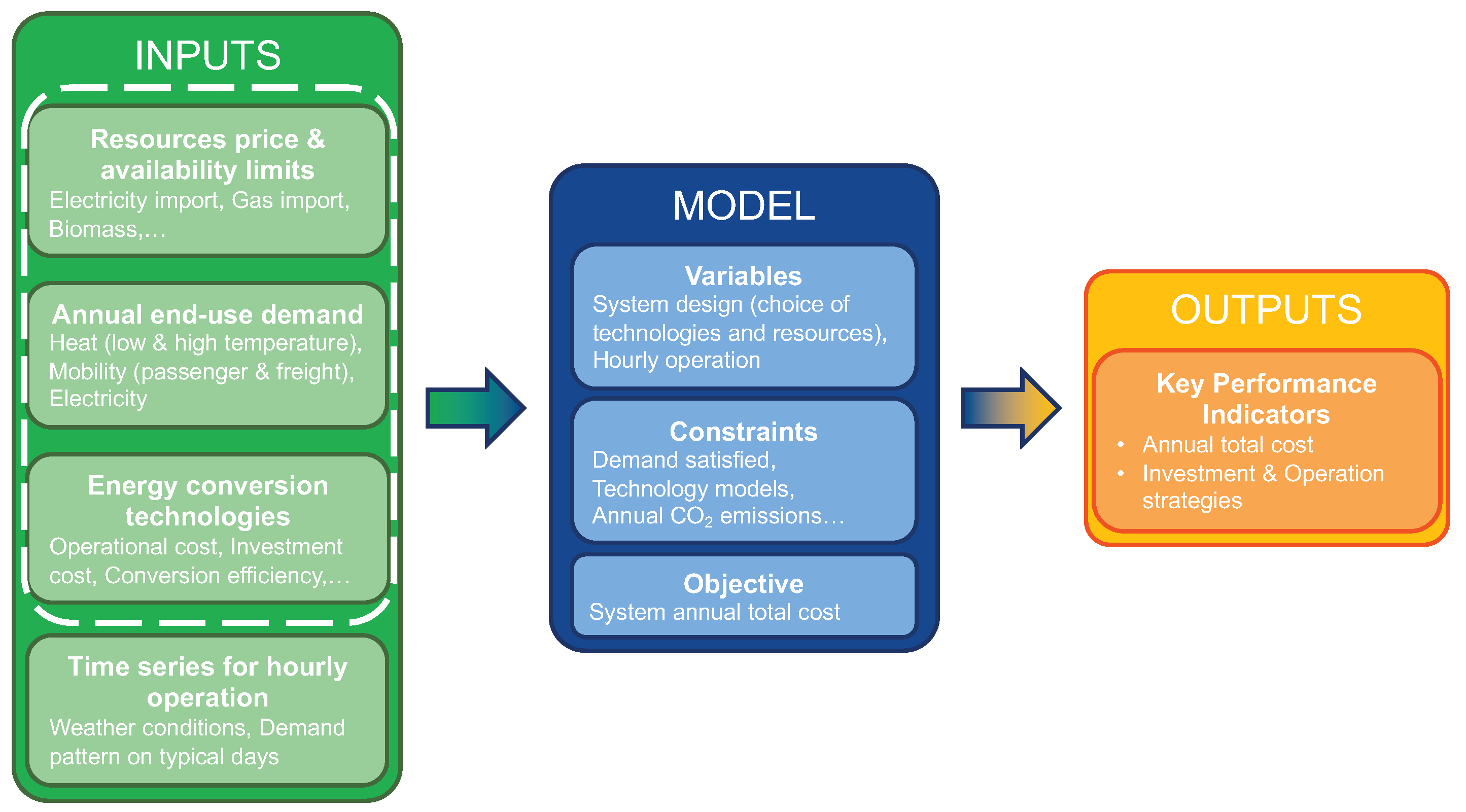
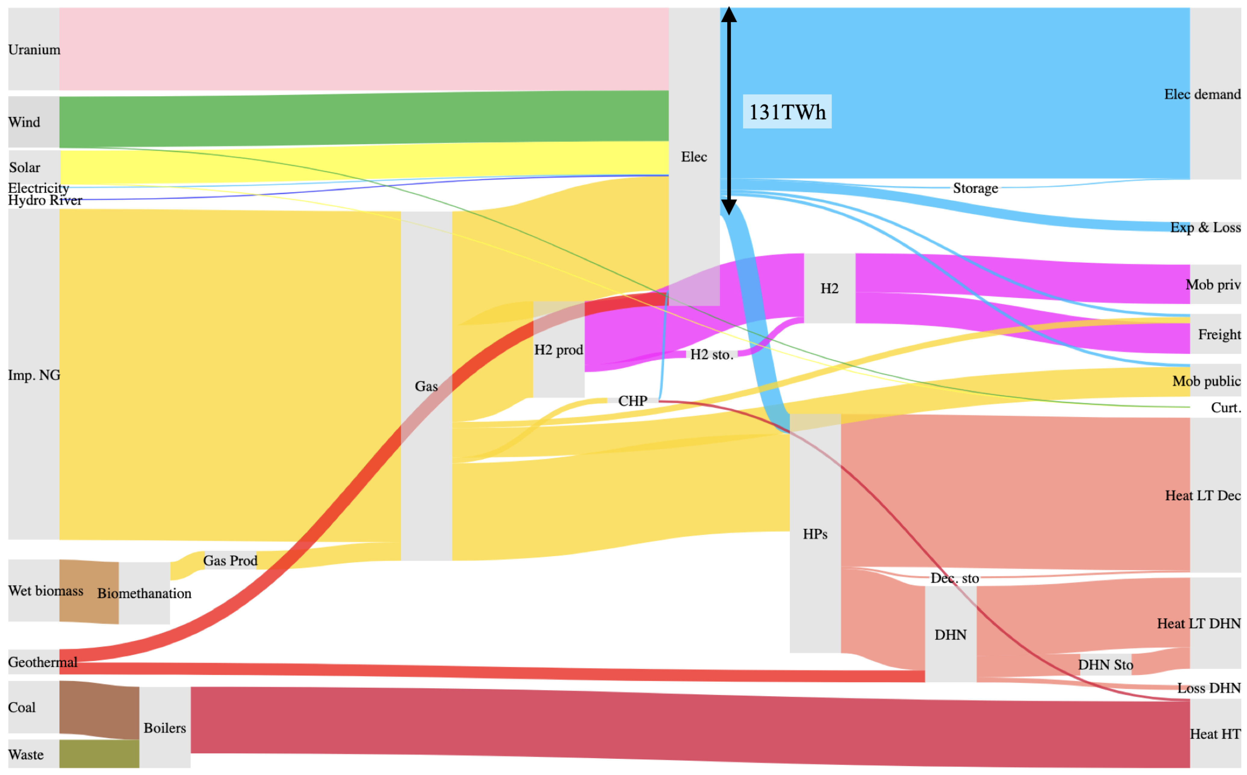

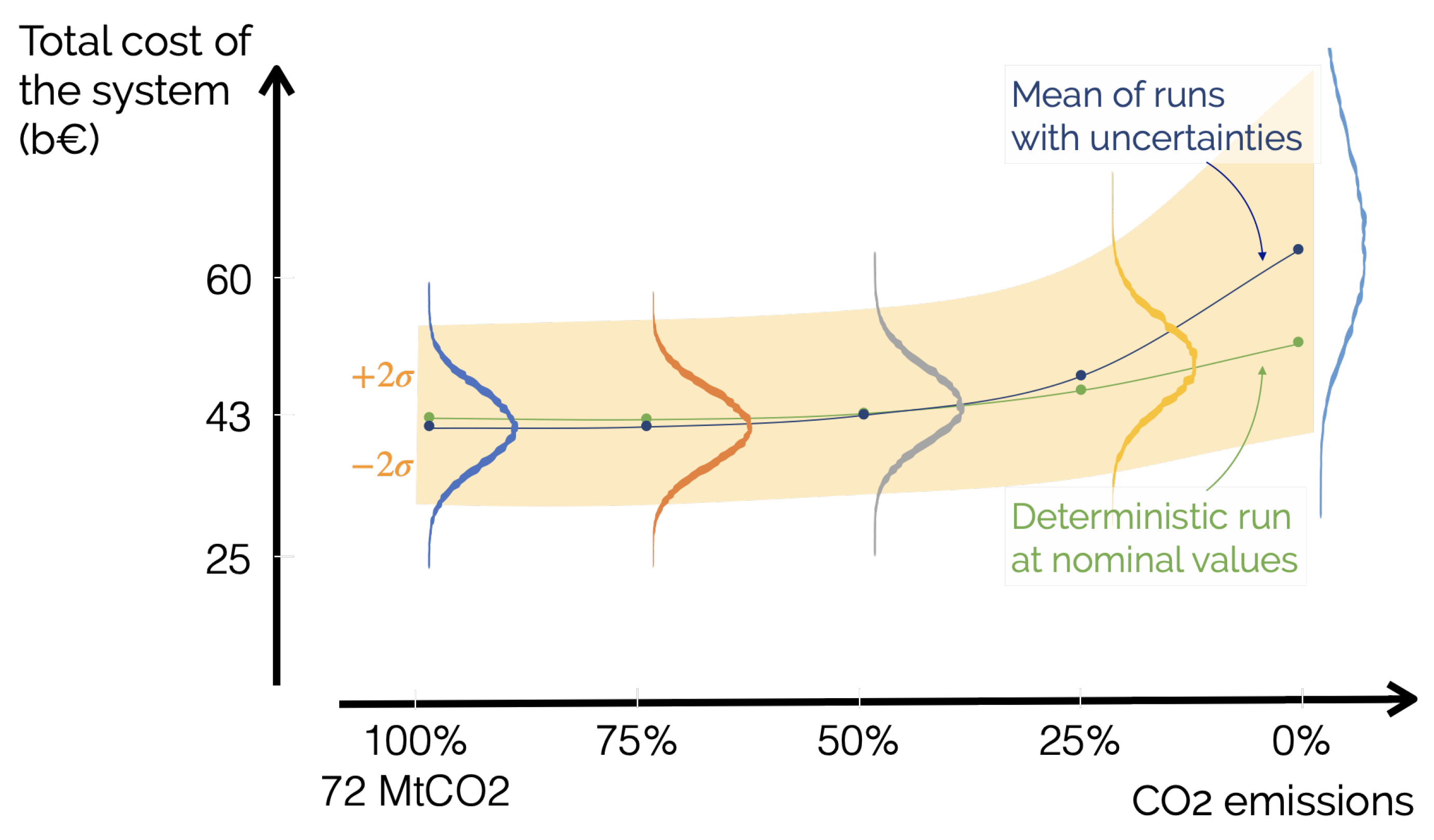
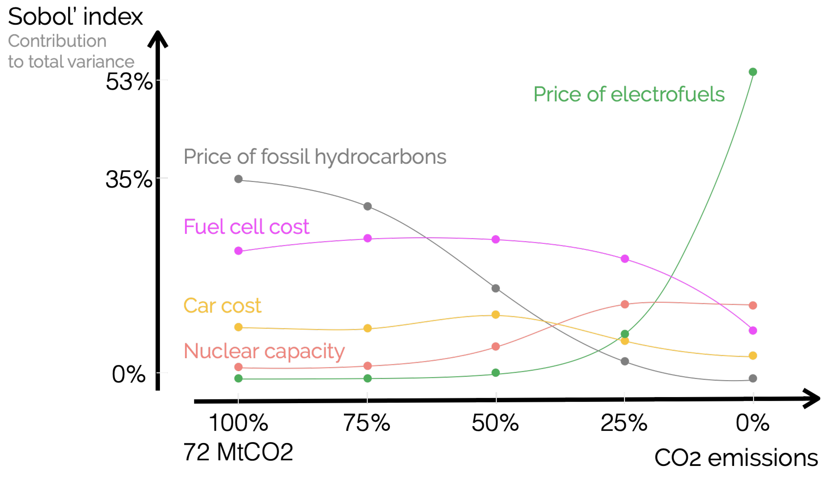
Publisher’s Note: MDPI stays neutral with regard to jurisdictional claims in published maps and institutional affiliations. |
© 2021 by the authors. Licensee MDPI, Basel, Switzerland. This article is an open access article distributed under the terms and conditions of the Creative Commons Attribution (CC BY) license (https://creativecommons.org/licenses/by/4.0/).