Article

Vehicle Energy Consumption in Python (VencoPy): Presenting and Demonstrating an Open-Source Tool to Calculate Electric Vehicle Charging Flexibility †

1
Department of Energy Systems Analysis, Institute of Networked Energy Systems, German Aerospace Center (DLR), Curiestr. 4, 70563 Stuttgart, Germany
2
Institute for Industrial Production, Karlsruhe Institute of Technology, Hertzstr. 16, 76187 Karlsruhe, Germany
*
Author to whom correspondence should be addressed.
This paper is an extended version of our paper published in 6th International Conference on Smart Energy Systems 2020, Aalborg, Denmark, 6–7 October 2020.
Energies 2021, 14(14), 4349; https://doi.org/10.3390/en14144349
Submission received: 14 June 2021 / Revised: 30 June 2021 / Accepted: 7 July 2021 / Published: 19 July 2021

Abstract

:
As electric vehicle fleets grow, rising electric loads necessitate energy systems models to incorporate their respective demand and potential flexibility. Recently, a small number of tools for electric vehicle demand and flexibility modeling have been released under open source licenses. These usually sample discrete trips based on aggregate mobility statistics. However, the full range of variables of travel surveys cannot be accessed in this way and sub-national mobility patterns cannot be modeled. Therefore, a tool is proposed to estimate future electric vehicle fleet charging flexibility while being able to directly access detailed survey results. The framework is applied in a case study involving two recent German national travel surveys (from the years 2008 and 2017) to exemplify the implications of different mobility patterns of motorized individual vehicles on load shifting potential of electric vehicle fleets. The results show that different mobility patterns, have a significant impact on the resulting load flexibilites. Most obviously, an increased daily mileage results in higher electricty demand. A reduced number of trips per day, on the other hand, leads to correspondingly higher grid connectivity of the vehicle fleet. VencoPy is an open source, well-documented and maintained tool, capable of assessing electric vehicle fleet scenarios based on national travel surveys. To scrutinize the tool, a validation of the simulated charging by empirically observed electric vehicle fleet charging is advised.

1. Introduction

Electric vehicles (EVs) have a widely accepted, published and well-understood technical potential of shifting their respective electric load for battery charging [1]. In energy systems analysis, different methods to estimate this potential have existed for many years [2].
As energy systems analysis models are oriented based on broader geographical and temporal scopes, they usually do not explicitly describe individual vehicles, power lines or transformers but focus on the integrative quality of EV fleets for photovoltaic and wind power feed-in in the context of long-term energy scenarios [3]. In such analyses, the focus is mainly on the power system impact of EVs, especially regarding peak loads and charging flexibility [4]. While open source tools to simulate EV charging have already been published, they mostly rely exclusively on sampling trips from mobility statistics.

1.1. State of Research

Transport and energy systems analysis approaches have been combined and compared in [5] to analyze the effects of different model details and the respective implications on energy systems optimization model results.
Although extensive research has been carried out on the effect of EVs for renewable energy (RE) integration, only a few tools have been publicly released that provide the flexibility needed to serve as data input generators for macro-scale energy systems modeling. However, in the last few years two tools have been released, which are briefly described in the following, as well as tools that are described below but are not available to reproduce scientific results.
RAMP-mobility is a stochastic generator for electric loads of single EVs [6]. Building on the broader RAMP-framework for stochastic multi-energy load profiles, it incorporates national specifics such as EV user types (students, workers or retired people), differences between vehicle sizes, and thus battery sizes, and specific consumption as well as stochastic effects of non-deterministic mobility behavior. RAMP-mobility calculates annual profiles in a minute-resolution taking also into account seasonal effects such as holiday travel and temperature-dependency of EV consumption. Three charging strategies can be simulated: uncontrolled charging, nighttime charging and RE sources integration charging. The tool has been validated against data gathered from ElaadNL with a resulting root mean square error of around 15% [7].
Emobpy is also a stochastic EV load generator taking into account user-specific probabilities of undertaking trips for shopping, work or other purposes, as well as location-specific probabilities for the charging infrastructure availability [8]. It follows a similar pattern, consisting of sampling trips throughout the time horizon to specific times of the day and incorporating consistency checks to ensure the vehicles can reach the household within the trip while being able to drive the specified daily trips with the available battery capacity. It has been applied in conjunction with the Dispatch and Investment Evaluation Tool with Endogenous Renewables (DIETER) specifying around 200 profiles, which serve as representative data basis for energy systems modeling [9].
Other methods have been described in the literature but are so far not available to researchers in open source licensed repositories and can thus neither be scrutinized by other researchers nor can their respective results be reproduced. The commercial tool synPro developed by the Fraunhofer Institute for Solar Energy Systems (ISE) and commercially applied by elink solutions focuses specifically on household electricity, heat and mobility demand [10]. The load flexibility tool eLoad of the Fraunhofer Institute for Systems and Innovation Research (ISI) has been formally well described [11]. It explicitly models arrivals and departures of vehicles of the grid-connected EV fleet increasing and decreasing the aggregate fleet battery and charging capacity. MobiFlex, the Matlab-based tool by KIT builds on the mobility patterns of the German mobility panel survey and has been demonstrated in the assessment of the RE curtailment reduction potential of electric fleets in the German federal state of Schleswig–Holstein [12].
The tool by the Fraunhofer Institute for Energy Economics and Energy System Technology (IEE) takes a decisive role in the range of EV fleet flexibility tools. Mobility groups form the core categories of the tool are modelled, being defined by population density categories, household size and household income. It differs from the above-mentioned tools in that it provides results for two analytical levels of abstraction [13]. On the one hand, it provides high-level EV fleet flexibility, on the other hand, characteristic user group-specific mobility patterns can be mapped to real-world household characteristic distributions in the context of distribution grid planning.
Energy systems analysis studies have been using national travel surveys for quite some time. Babrowski et al. analyze different EV load shifting scenarios based on national travel surveys of Denmark, Germany, Finland, The Netherlands, Switzerland and the United Kingdom [1]. For Germany, this method is applied in grid analysis in [14].
The predecessor of the tool described here, the tool VENCO (Vehicle Energy Consumption) was originally developed and applied in [3]. De Tena and Pregger use VENCO to derive consumption patterns for battery EVs, hybrid EVs and fuel cell EVs in a European scenario study [15].
As already mentioned, methods simulating EV charging flexibility have been developed, formally described and in some cases made available under an Open Source license. However, most tools go unnoticed and the ones that are formally described are mostly undisclosed while the two rare cases of published code repositories follow sampling approaches from national travel surveys rather than discrete trip diary compositions. The last point is specifically important to researchers who are interested in only a subset of survey respondents e.g., a specific federal state, socioeconomic status or vehicle size.

1.2. Contribution

A tool including interfaces, filtering and cleaning routines of national travel surveys together with methods for simulating EV load shifting potential is developed. The tool Vehicle Energy Consumption in Python (VencoPy) aims at filling a gap for researchers that have access to national travel survey data, potentially in high geographical and temporal resolution. In the following chapters, both a formal description of all algorithms of the tool as well as a reference to the codebase on gitlab [16] are provided. To demonstrate the capabilities of the tool, a case study is presented, which analyzes two German national travel survey data sets: The Mobility in Germany 2008 (in German: Mobilität in Deutschland, MiD08) and its recent update from 2017, the MiD 2017 (MiD17). The case study shows how differences in mobility patterns transfer to differences in EV charging, connection and consumption patterns in a scenario setup with vehicle battery sizes assumed to be 50 kWh and an average electric consumption of 20 kWh/100 km. Effects of differences in travel behavior on EV charging patterns have been assessed before between different European countries [1], but no analyses have presented changes within a country between different years yet.
VencoPy is compared to the body of existing literature in the field by comparing its simulation results to previously documented values for EV fleet power, respective patterns and charged energy.
The insights provided by VencoPy are valuable mainly to energy systems analysts in need of EV data adjusted to model-specific scopes as well as transport researchers interested in the effects of mobility patterns on potential charging flexibility of EV fleets. Additionally, the term EV in this context only refers to individual battery EVs.
The paper is structured as follows. Section 2 introduces the proposed and published fleet estimation calculations. Section 3 compares the main mobility patterns of the two analysed samples—MiD08 and MiD17. Most of the findings until this section reproduce or further detail findings already described in [17,18]. Subsequently, the results of an electric fleet what-if-analysis based on 2008 and 2017 data sets are presented to demonstrate VencoPy’s simulation capabilities. Finally, conclusion and critical reflections on the used approach are drawn in Section 4.

2. Materials and Methods

Since VencoPy’s predecessor VENCO applied in [3] and in [15] as early as 2010 has neither been formally described nor published, a comprehensive formal representation of the EV fleet charging flexibility estimation procedure is presented here.

2.1. VencoPy Structure

Figure 1 shows the detailed VencoPy components in a developer diagram. The four components—implemented as Python classes—DataParser, TripDiaryBuilder, GridModeler and FlexEstimator can be clearly distinguished. A fifth component, Evaluator, used to create the plots for this work is not shown in Figure 1 as it is not needed to calculate results from VencoPy.
Following [19], VencoPy is described on four Levels of abstraction:
  • Linguistic description in plain English;
  • An algebraic formulation;
  • The model implementation in code;
  • A model application to a specific context.
Descriptions in this Section follow Levels 1 and 2. The code implementation can be retrieved from the open repository [16]. The application level is finally presented in Section 3. The difference between the first two levels and the third level consists mainly of the human–machine interfaces such as configuration files, technical interfaces between the input formats, internal variable declaration, formatting and translating the algebraic formulations in machine-readable Python statements. For more details, the technically interested reader is referred to the VencoPy documentation pages available via the readmefile of the repository [16].
Elements of independent variables for the following derivations are shown in Table 1. In its current version, VencoPy only differentiates the vehicle sizes via the battery and consumption assumptions but not in the mobility patterns. The same is true for propulsion technologies. For the application of VencoPy results in energy systems models, the boundary conditions on the individual profile levels assure that the beginning t = 0 and end t = T values match.

2.1.1. Interface to the Dataset: DataParser Class

The first step in the VencoPy framework to be able to estimate EV energy consumption implies accessing a travel survey data set, such as the MiD [17]. This is carried out through a parsing interface to the original database. In the parsing interface to the data set, three main operations are carried out: the read-in of the travel survey trip data, stored in .dta or .csv files, filtering and cleaning of the original raw data set and a set of variable replacement operations to allow the composition of travel diaries in a second step.
In order to have consistent entry data for all variables and for different data sets, all database entries are harmonised, which includes generating unified data types and consistent variable naming. The naming convention for the variables and their respective input type can be specified in the VencoPy-config files. A full list of the required variables is provided in Table A1. Of the 22 variables, four variables are used for indexing, 11 variables characterise the trip time within the year, two variables are used for filtering and five variables characterize the trip itself. The representation of time may vary between travel surveys.
Starting from the initial raw trip record base set D tot , a subset data set D sel is created after filtering irrelevant entries or those that lack necessary information.
D tot = { 1 , , r } N ; D sel D tot
For every trip data record in D sel , four filters are applied for cleaning purposes. The first two filters employ inclusion and exclusion conditions for specified discrete variables. Exclusion filters are mainly used to clean out incomplete variable values. For every trip data record, r, in D sel , the inclusion and exclusion filters can be written as
filter 1 ( include ) : v a r i a b l e N a m e r = v a l i d R e c o r d V a l u e D sel r D tot
filter 2 ( exclude ) : v a r i a b l e N a m e r = i n v a l i d R e c o r d V a l u e D sel r D tot
Additional two filters set upper and lower boundaries for continuous variables, such as mileage, as follows:
filter 3 ( upper bound ) : v a r i a b l e N a m e r < u p p e r B o u n d a r y V a l u e D sel r D tot
filter 4 ( lower bound ) : v a r i a b l e N a m e r > l o w e r B o u n d a r y V a l u e D sel r D tot
Most travel surveys include motorized, non motorized as well as multi-modal trips. For the scope of VencoPy, only trips that were carried out with a motorized individual vehicle are selected. To exemplify the application of the filters described above, this implies that Equation (2) for the variable named ’driver’ equals 1 ( d r i v e r r = 1 r D sel ), which means that the person who carried out the r-th trip was the driver of the vehicle, i.e., it is a motorized trip. Similarly, trips with missing (e.g., missing tripID, missing start or end time etc.) or invalid information (e.g., implausible trip distance) are filtered out. Filters can be easily adapted to other travel survey numeric codes via the config-file.
By applying the set of filters described in Equations (2)–(5), the initial database is subset to only contain valid entries representing motorised trips. The last operation in the parsing of raw travel survey data sets is a harmonization step.

2.1.2. Daily Travel Diary Composition: TravelDiaryBuilder Class

In the second VencoPy component, the travelDiaryBuilder, individual trips at the survey day are consolidated into person-specific travel diaries comprising multiple trips.
The daily travel diary composition consists of three main steps: reformatting the database, allocating trip purposes and merging the obtained dataframe with other relevant variables from the original database.
In the first step, reformatting, the time dimension is transferred from the raw data (usually in minutes) to the necessary output format (e.g., hours). Each trip is split into shares, which are then assigned to the respective hour in which they took place, generating an hourly dataframe with a timestamp instead of a dataframe containing single trip entries.
Similarly, miles driven and the trip purpose are allocated to their respective hour and merged into daily travel diaries. Trips are assumed to determine the respective person’s stay in the consecutive hours up to the next trip and therefore are related to the charging availability between two trips. Trip purposes included in surveys may comprise trips carried out for work or education reasons, trips returning to home, trips to shopping facilities and other leisure activities. Currently, trips whose purpose is not specified are allocated to trips returning to their own household.
A detailed visualized description of the steps on the first abstraction level is given in Appendix B.
At the end of the second VencoPy component TripDiaryBuilder, two intermediary data sets are available either directly from the class within Python or from the hard-drive as .csv files. The first one comprises mileage travel diaries d ( v , t ) and the second one comprises parking place types derived from trip purposes p a r k i n g T y p e ( v , t ) .

2.1.3. Charging Infrastructure Allocation: GridModeler Class

The charging infrastructure allocation makes use of a basic charging infrastructure model, which assumes the availability of charging stations when vehicles are parked. Since the analytical focus of the framework lies on a regional level (NUTS1-NUTS0), the infrastructure model is kept simple in the current version.
Charging availability is allocated based on a binary True–False mapping to a respective trip purpose in the VencoPy-config. Thus, different scenarios describing different charging availability scenarios, e.g., at home or at home and at work etc. can be distinguished, but neither a regional differentiation nor a charging availability probability or distribution are assumed.
At the end of the execution of the GridModeler class, a given parking purpose diary p a r k i n g T y p e ( v , t ) is transferred into a binary grid connection diary c o n n e c t grid ( v , t ) with the same format but consisting only of True–False values.

2.1.4. Flexibility Estimation: FlexEstimator Class

There are three integral inputs to the flexibililty estimation:
  • A profile describing hourly distances for each vehicle d ( v , t ) ;
  • A boolean set of profiles describing if a vehicle is connected to the grid at a given hour c o n n e c t grid ( v , t ) ;
  • Techno–economic input assumptions described above and further specified in Table 2.
This yields the minimum and maximum battery constraints, which are calculated as:
C bat , min = C bat × m a r g min
C bat , max = C bat × m a r g max
The electricity flow from the battery to the electric motor for each EV in each hour is calculated by multiplying the driven distance by an assumed average specific electric consumption c o n s elec in kWh 100 km :
d r a i n elec ( v , t ) = d ( v , t ) × c o n s elec / 100
p charge , max ( v , t ) = c o n n e c t grid ( v , t ) × p charge
For t = 0 , the following case differentiation assures that the battery SoC of each mobility profile stays below S o C max and that the following boundary condition is enforced for each individual profile:
S o C max ( v , t = 0 ) = S o C max ( v , t = n hour 1 )
S o C max ( v , t ) = (11) S o C max ( v , t = n hour 1 ) if S o C max C bat , max (12) C bat × m a r g max else
For t > 0, the following new SoC is calculated. Additionally, it is assured that S o C new stays within the battery limits through:
S o C max , new ( v , t 0 ) = S o C max ( v , t 1 ) + p charge , max ( v , t ) d r a i n elec ( v , t )
S o C max ( v , t 0 ) = (14) C bat , min if S o C new ( v , t ) < C bat , min (15) S o C max , new ( v , t ) if C bat , min S o C max , new ( v , t ) C bat , max (16) C bat , max if S o C new ( v , t ) > C bat , max
Since differences at the profile boundaries should be minimized, Equations (10)–(16) are iteratively executed until a predefined number of iterations is reached. The user is displayed the sum of differences of the SoC values for t = 0 and t = n hour 1 over all profiles:
i t e r a t i o n C h e c k s u m max = v = 0 V 1 S o C max ( v , t = n hour 1 ) S o C max ( v , t = 0 )
Then, uncontrolled charging is calculated as the profile that occurs when vehicles connect as soon as possible and charge with the maximum capacity available at that point in time. For brevity, the dependence on v is left out in the following case differentiation.
C unc ( v , t 0 ) = (18) S o C max ( t ) S o C max ( t 1 ) if S o C max ( t ) S o C max ( t 1 ) (19) 0 else
For t = 0 , a proxy approach is chosen:
c unc ( v , t = 0 ) = c unc ( v , t = 1 ) + c unc ( v , t = n hour ) 2
The fuel demand for trips with a mileage beyond electric mileage is calculated via Equations (21) and (22) as:
d r a i n fuel ( v , t 0 ) = c o n s fuel c o n s elec * d r a i n elec ( v , t ) c unc ( v , t ) S o C max ( t 1 ) S o C max ( t )
d r a i n fuel ( v , t = 0 ) = d r a i n fuel ( v , t = 1 ) + d r a i n fuel ( v , t = T ) 2
The demand-sensitive minimum SoC of each vehicle is calculated taking into account the profiles from Equations (18)–(22). Analogous to Equation (10), the following is enforced:
S o C min ( v , t = 0 ) = S o C min ( v , t = n hour 1 )
S o C min ( t = n hour 1 ) = (24) S o C min ( t = 0 ) if S o C min ( t = n hour 1 ) C bat , min (25) C bat , min else
For t > 0, the following new SoC is calculated. Additionally (27) assures that S o C new stays within the battery limits. For brevity, the dependence on the specific vehicle is not written.
S o C min , new ( t n hour 1 ) = S o C min ( t + 1 ) + d r a i n elec ( t + 1 ) p charge , max ( t + 1 ) d r a i n fuel ( t + 1 ) × c elec c fuel
S o C min ( t n hour 1 ) = (27) C bat , min if S o C min , new ( t ) < C bat , min (28) S o C min , new ( t ) if C bat , min S o C min , new ( t ) C bat , max (29) C bat , max if S o C min , new ( t ) > C bat , max
Since differences at the profile boundaries should be minimized, Equations (23)–(29) are iteratively executed until a predefined number of iterations is reached. The user is displayed the sum of differences of all profiles.
i t e r a t i o n C h e c k s u m min = v = 0 V 1 S o C min ( v , t = n hour 1 ) S o C min ( v , t = 0 )
After these steps, the six profiles shown in Table 3 are provided to the user.
The first four profiles can be used as constraints for other models to determine optimal charging strategies; the fifth profile simulates a case where charging is not controlled an EVs charge as soon as a charging possibility becomes available. Lastly, the sixth profile quantifies the demand for additional fuel for trips that cannot be fully carried out with an EV.

2.1.5. Filtering

Four filters are applied in the following to these profiles. The first filter excludes profiles that need fuel. The user can give a tolerance level to keep profiles in the data basis for consecutive steps. This filter is applied when only EV profiles should be calculated.
filter 1 ( v ) : t = 0 T 1 d r a i n fuel ( v , t ) < t o l e r a n c e fuel v V
The second filter requires a random number r ( v ) between 0 and 1 for each profile and is calculated as follows:
filter 2 ( v ) : t = 0 T 1 d ( v , t ) > 2 × r ( v ) × d min + ( 1 r ( v ) ) × d min v V
d min is a global parameter of VencoPy that the user can freely adjust to manipulate the profiles for selecting either rather EV-prone profiles or rather longer-range profiles.
The third and fourth filter are additional filters to limit the amount of profiles that are taken into account as described in Equations (33) and (34).
filter 3 ( v ) : t = 0 T 1 d r a i n elec ( v , t ) < t = 0 T 1 p charge , max ( v , t ) v V
filter 4 ( v ) : t = 0 T 1 d r a i n elec ( v , t ) < S o C bat , max S o C bat , min v V
The user is displayed information on how many profiles were filtered out and how many are still part of the data.
The electric demand for driving is reduced by the share of fuel combustion to power the battery in order to gain the net electric battery outflow per hour:
d r a i n elec , net ( v , t ) = d r a i n elec ( v , t ) d r a i n fuel × c fuel c elec

2.1.6. Normalization

The SoC profiles are normalized to the respective battery capacities in order to produce comparable profiles.
S o C min , norm ( v , t ) = S o C min ( v , t ) C bat

2.1.7. Aggregation

In order to draw conclusions on EV fleets, aggregation of the individual profiles to EV fleet level is performed. In its current version, this is done for the whole set of data and different vehicle sizes are not differentiated due to the missing allocation of trip data (which is only referenced by household and person but not by vehicle) to vehicles and thus vehicle sizes.
For all four flow profiles f ( v , t ) aggregation is carried out via:
f ( t ) = v = 0 V 1 f ( v , t ) V
For the two state profiles S o C ( v , t ) aggregation is carried out by selecting the n th largest or smallest value of the profile in each hour for S o C max ( v , t ) and S o C min ( v , t ) , respectively. With α being between 0 and 1, the “n” of n t h element [15] and V being the total number of profiles, the limiting value is calculated as:
v limit = α × V
De Tena describes 1 v limit as the confidence interval. Thus when α = 5 , this results in a confidence interval of 95% where the SoC limitations fulfil the needs of 95% of the assessed trips [3]. After this, S o C min , limit ( t ) and S o C max , limit ( t ) , the threshold SoC values are calculated for each hour. To satisfy the demand of the entirety of vehicles in the confidence interval, the fleet SoC must not surpass this threshold SoC.
S o C min , limit ( t ) = min n = v limit ( n largest ( S o C min , limit ( t , v ) ) )
S o C max , limit ( t ) = max n = v limit ( n smallest ( S o C max , limit ( t , v ) ) )
where n largest ( ) and n smallest ( ) are the operations to select for example the 95% largest or smallest values of a set of values.

3. Results

After describing the more recent of the two data sets in greater detail, the resulting mobility profiles with and without weekday differentiation are analysed. On this analytical level the effect of applying the trip weights to account for trips being more or less representative for overall travel behavior within the sample population are visualised. These analyses mainly reproduce findings from [17] for MiD17 and from [18] for a comparison of MiD08 and MiD17. However, since the interest here mainly lies in temporal differentiations, only the effects of the already described changing patterns on the traffic volume in high temporal detail are described.
Secondly, the flexibility estimation of VencoPy is demonstrated by showing how differences between two travel surveys propagate to simulation results. The case study is limited to battery EVs, so Equations (21) and (22) and the resulting profile d r a i n fuel ( v , t ) are disregarded.

3.1. Case Study Data

The latest German national travel survey “Mobilität in Deutschland” (MiD17) was carried out in the years 2016 and 2017. Mobility patterns for one randomly chosen day per survey participant were collected across Germany. The survey was carried out as a multiple frame survey, taking into account three samples gathered across Germany and 55 regional samples of participating federal states and counties. For comparison, trip data from the predecessor survey-“Mobilität in Deutschland 2008” (MiD08)-are taken into account [20].
The MiD17 data set can be accessed in four different degrees of detail with A being the overall national aggregates disclosed to everyone and from B1 to B3 being the datasets with an increasing spatial detail. The dataset used in this analysis is the MiD B2 dataset, which contains information on county level. The B2 dataset consists of the three tables households, person and trips, connected via unique household-ID, person-ID and trip-ID. Only 22 of the 157 variables given for each trip are used since the interest only lies in vehicle mobility and their most relevant variables, thus making the application of VencoPy easier for other national travel surveys. Examples of provided variables that are not relevant for the technical analytical steps described here but may be accessed for consecutive analyses (before aggregation) are federal state, region type, economic household status, age groups or boolean variables referring to the transport mode. Still, users can access the full range of information not only of the trips but also of households and persons through merging the IDs within the initial original data set.
The data set is described in multiple documents of which only the study summary and short report are available in English. More detailed descriptions are available in German in the final report [17], the travel survey user handbook [21], the method report [22] and the time series report [18].
Starting from the initial raw trip record base set D tot , containing around 961,000 entries, a subset data set D sel is created after filtering invalid entries, resulting in slightly more than 400,000 database entries for individual trips. This reduction to less than 50% of the data set is mainly due to selecting only trips carried out by motorized individual vehicles and minor consistency cleaning steps.
For the trip data of the MiD17, the average travel time lies at one hour and 20 min as the total average over the entire dataset and one hour and 34 min for single persons, i.e., persons that carry out at least one trip on the survey day. It significantly depends on age, employment, and population density and is only slightly affected by gender (males survey respondents travel five minutes more on average than female ones).
The number of trips lies at 3.1 trips/day on average for the whole dataset and 3.7 trips/day for single persons. The number of trips, as well as the trip purposes, are not affected by population density or differences across Germany. However, the length, times or other specifics of these trips differ [17]. Seasonal differences are marginal with regard to the number of trips per person and day. However, weekdays strongly influence this metric. Trips occur more often on workdays than on weekend days with their minimum on Sundays with an average of 2.1 and 2.8 trips per person/day for the whole dataframe and single persons respectively.
Daily travel distance is the most variable metric on average. It differs by 10 km between densely populated regions vs. metropolitan regions. Seasonal effects for this metric are much more pronounced than for the number of trips. The daily travel distance ranges between 42 km in winter and 48 km in summer on average for single persons in the overall sample. The influence of weekdays on average daily travel distance differs from the influence on other metrics. Daily travel distances are lowest on Tuesdays and Wednesdays and rise towards the weekends (Mondays and Thursdays) to 44–45 km/day, respectively. Regarding this metric, Friday with its 50 km/day has a similar characteristic as Saturday (48 km/day) and the weekday maximum Sunday (52 km/day). Sunday’s specific travel characteristic is also mirrored in the average trip length of 18 km/trip, which differs significantly from the 11–13 km/trip throughout the other days.
Table 4 shows the analyzed metrics for the overall MiD08 and MiD17 populations and for the filtered sample containing trips carried out by vehicles ( D sel subset).
Other influences that were part of the survey such as the influence of gender, economical status and employment type are excluded from the detailed analysis but are a fruitful starting point for further analysis, especially on geographically smaller areas. Since VencoPy has the foremost application context of providing information for European-wide energy systems models on a scale of federal states (3–7 Mio. inhabitants) to national regions, these influences are assumed to be negligible for the research questions at this scale. However, especially for transferring insights to other European countries, some of these measures (especially distribution of economical status, employment type and age) are promising for hypothesis building or preliminary assumptions in the case of lack of detailed national travel survey data.

Weights in the German National Travel Survey Data Set

One of the goals of the MiD is to provide aggregate statistics of German mobility. In order to do so, households, persons and trips are associated with weights describing the representativeness of a respective observation. Here, only the trip weights are considered since they comprise all necessary information to calculate trip aggregates from trip samples. Since the survey has a variety of heterogeneous selection frames, an estimator such as the Horvitz–Thompson estimator has to be applied in order to scale variables from the sample to the entirety of the German society [21]. In this regard, the steps described in [22] are followed for the scaling from the sample population to the entirety of the German population.

3.2. Case Study Results: Mobility Patterns

As described above, several steps are taken in order to calculate average profiles for entire fleets. In this paper, no results for a scenario study of 2030 or similar, as done with VencoPy in [5], are shown but the interest is rather focused on all resulting profiles on the level of the average vehicle, thus providing a basis for scaling to any fleet size.
Figure 2 shows the mobility patterns for an average vehicle in Germany differentiated by the weekday. The top plot shows the larger sample size of the MiD2017 due to its additional regional in-depth samples that were realized for the first time [22]. The bottom plot shows the effect of the increased average trip distance already shown in Table 4. Weighting has a marginal influence for average daily mobility based on the MiD08, but reduces the daytime distance travelled based on MiD17 accounting for over-represented high-distance travellers on Saturday–Monday in the sample.
Traffic volume is higher in the MiD17 specifically on weekend days, most pronounced on Sundays and moderately higher on Fridays and Mondays. While average hourly distances are comparable based on MiD08, mobility patterns show a clear increasing trend from Fridays through Saturdays and peaking on Sundays at approximately 12.5 km/h around 12:00 on average. This dynamic although already present in the MiD08 sample is more evident from the MiD17 sample.

3.3. Case Study Results: Flexibility Estimation

In the following, results of the flexibility estimation are shown which consider weights in the aggregation process from individual profiles, e.g., for uncontrolled charging, to the estimated average EV profiles. As shown in Table 3, this flexibility is described by the four profiles’ battery drain d r a i n elec ( t ) , maximum charging capacity p charge , max ( t ) as well as minimum ( S o C min ( t ) ) and maximum SoC ( S o C max ( t ) ). A fifth profile, uncontrolled charging c h a r g e unc ( t ) , is calculated as well, assuming vehicles are charged as soon as a grid connection is available.
Figure 3 shows the counteracting effects of increased travel distances in a lower number of trips [18]. Charging is available when vehicle owners are at home which is mainly during the morning, evening and night. While daytime grid connection shares are higher based on the MiD17 data set during workdays, the opposite is the case in a milder intensity for the weekend. This can be explained by almost doubling average trip distance travelled on Sunday, compensating for less trips being carried out. However, as described above, this effect is small compared to the overall change in fleet grid connection share.
Compared to the differences in fleet grid connection shares, changes in mobility patterns imply stronger changes in electricity outflow from the battery for driving as depicted in Figure 4 since mobility changes directly translate into drain changes. Increased average trip distance travelled between 9:00 and 17:00 leads to increased electricity consumption for driving mainly from 8:00 to 17:00. In its peak at 16:00, the average electricity consumption is 0.3 kWh/h based on MiD08, whereas it is 0.55 kWh/h based on MiD17.
The average electricity consumption for driving shows characteristic morning and evening peaks throughout the week. The maximum in fleet consumption for driving d r a i n elec ( t ) can be observed for evenings with approximately 0.6 kWh/h per vehicle on average. Increased average trip distance in MiD17 compared to MiD08 leads to higher electricity consumption at almost every hour. Sunday differences in consumption are higher by almost a factor of 2, from 0.35 kWh/h to 0.7 kWh/h on average. Saturdays show a broader travel characteristic during daytime the but peaking below Tuesday evening travels.
Uncontrolled charging shown in Figure 5 differs between the two samples in the time interval between 16:00 and 21:00 with its peak at 18:00. In this peak, c h a r g e unc ( t ) results in 0.5 and 0.8 kW for MiD08 and MiD17, respectively. The patterns in the uncontrolled charging scenario are thus quite similar.
The trends described for an average day are mirrored by weekly EV fleet uncontrolled charging. The peak broadened a bit and increased in size from under 0.6 to 0.8 kW. On Fridays and Saturdays uncontrolled charging is more distributed throughout the day with increasing peaks in the evenings. Sundays show the all-week high slightly below 1 kW on average, this having increased more than two-fold showing the stark travel increase on Sundays between the MiD08 and MiD17.
SoC profiles shown in Figure 6 depict a temporally dependent average battery range for load shifting. This battery range is reduced by a reduced maximum SoC and an increased minimum SoC at daytimes when vehicles on the road cannot charge but need a minimum of SoC for the planned trip on that respective day.
The average vehicle SoC is smaller for the estimation based on the MiD17 dataset, which is due to increased travel distances in the sample. This reduction is most pronounced on Sundays when the two profiles almost touch, implying no charging flexibility for the average vehicle at all. Still, during nights, an average vehicle provides a large source of flexibility with the full accumulator capacity of 50 kWh available for flexible charging.
Simple methods for aggregating individual SoC profiles to fleet level as used here have been shown to overestimate the fleet load shifting potential. Mathematically correct methods exist but have been shown to currently be impractical on time horizons employed in the context of energy systems analysis (T > > 10 time steps) [2]. The given profiles can be a first indication for a vehicle fleet flexibility, however greater care in applying them in the context of evidence-based decision making should be taken.

4. Discussion

4.1. Situating VencoPy Simulation Results on the Background of Literature Results

Comparing VencoPy simulation results with results for EV fleet charging given in the literature is difficult due to different boundary conditions such as assumed battery capacities and specific electricity consumption and infrastructure modeling detail. Still, the results presented above are described next to literature findings of three studies, even though a direct comparison cannot really be performed. Two of the studies follow a similar approach extrapolating fossil fuel vehicle mobility behavior to electric fleets [12,23] and a third one assessing empirically measured charging events [24], thus being more heterogeneous in the vehicle model range and used infrastructure. Table 5 gives an overview of the studies and assumptions.
All profiles are compared on the basis of an average vehicle of the fleet on the basis of charging power and respective patterns throughout the day as well as the volume of charged energy as an aggregate measure.

4.1.1. Power and Patterns

Electricity consumption and uncontrolled charging power values are similar to literature values. VencoPy calculates electricity consumption values between 400 and 500 W for morning peaks at 7:00 and 500 and 600 W for evening peaks at 16:00 on workdays. On the weekend, electricity consumption peaks at 500–700 W around noon. Only Heinz provides electricity consumption estimates peaking at 500–550 W at 7:30 and 17:00 on average on workdays and at 400 W at 15:30 on weekend days [23].
VencoPy simulations yield uncontrolled charging evening peaks amounting to 700–800 W on workdays and 600–950 W on weekend days on average occurring at 18:00. Comparing evening peaks for uncontrolled charging, Ried finds evening peaks of 870 W on workdays and 480–550 W on weekend days peaking at 19:00–20:00 and 19:00, respectively [12]. Heinz finds peaks of 560 and 340 W occurring at 18:00 and 18:30 for workdays and weekend days, respectively [23]. Schaeuble et al. report a peak of 380 W on 18:15 on an overall average day, standardizing the profiles with an own calculation of daily charged energy based on the average daily driven distance of 39 km given in MiD [24].
Grid connection shares are given only by Heinz describing around 1.75 kW of 3.5 kW (50%) at its minimum occurring at 10:30 in the morning on an average workday for the home charging scenario [23]. On the weekend the minimum connected power increases to 2.7 kW (77%) at 11:00. VencoPy’s grid connection shares are reduced to 40% on workdays and 55–70% on weekend days. The results are thus slightly lower throughout the week suggesting that the dataset used describes more mobile vehicle users.

4.1.2. Charged Energy Volumes in the Uncontrolled Charging Scenario

The total amount of energy charged is compared to two values. For one, ref. [24] discusses different daily energy volumes charged in the evaluated empirical data sets on the background of rule-of-thumb calculations using average distance travelled. The latter yields a charged energy of 5.4 kWh per day including losses compared to 4.4 kWh and 9.2–11.5 kWh depending on the respective measured data set with the latter’s variation stemming from different weekdays. Heinz’s published profiles enable a reproduction of charged energy for the calculated representative profile [23]. Assuming discretised 10-min power values yields average charging volumes of 4.9 kWh/day on workdays and 3.6 kWh/day on weekend days. VencoPy’s charged energy demand for uncontrolled charging lies slightly higher with 5.4 kWh/day for the average vehicle at an average day than values from [23] but well in the range given in [24]. Two times higher values for daily charged energy volumes reported for the Get eReady study carried out between 2013 and 2015 in Stuttgart can be explained by non-representative vehicle users as 75% of survey participants were small to medium sized companies receiving a refund for their participation.

4.2. Limitations and Potential Improvements

A potential improvement in a future charging flexibility estimation would be to take into account charging probabilities and to sample grid connections to trip purpose-dependent stays based on a given probability [8]. In a next step, further dependencies such as regional charging availability could be assumed.
Moreover, the decision to plug in a vehicle when a charging point is available is not explicitly modeled and it is assumed that users always connect their vehicles when charging is available. A potential improvement could be to incorporate fitted models given, for example, for the case of public charging in [25]. Energy system models usually require annual profiles in hourly or sub-hourly resolution. VencoPy currently only supports annual calculations which are structurally fixed in the tools codebase. Temporal resolutions down to at least 10-min intervals may be supported by the data used in the case study (MiD08 and MiD17). Furthermore, seasonal influences on drain profiles such as temperature changes have been suggested by other authors and should be incorporated into the tool.
Aggregated profiles for fleet state-of-charge profiles have been shown to exaggerate the flexibility potential of fleets. Mathematically exact Minkowski sums have been proposed as a mean of representing fleets’ aggregated load shifting potential, however applications to intervals greater than 2 h have been shown to be infeasible due to exponentially increasing calculations times.
The analysis of the mobility pattern is based on fossil fuel cars. There is evidence in the literature that EV users drive their cars differently. However, this change may currently be exaggerated with EV users still not being representative for the entirety of individual motorized vehicle users. However, future travel surveys may provide sufficient information to isolate EV users and thus run comparable analysis without this strong overarching assumption.

5. Conclusions

Changing mobility patterns described in detail by national travel surveys, such as ’Mobilität in Deutschland’ for Germany, may imply changes in EV fleet electric load shifting potential estimations. For the interval between 2008 and 2017, a slight decrease in the number of trips per day and person from 3.4 to 2.9 and a strong increase in unweighted average distance travelled from 9.4 to 17 km per person/day for motorized individual vehicles is evident from the analysis.
The Open Source tool Vehicle Energy Consumption in Python (VencoPy) makes use of an interface to the data, filtering and evaluation algorithms to assess the consequences of these changes in high temporal resolution for an average week.
In a what-if scenario assuming an EV battery size of 50 kWh, a specific consumption of 20 kWh/100 km, only home charging and a maximum charging power of 11 kW, the effects of these mobility pattern changes on the average EV flexibility are assessed.
Slight increases in fleet charging capacity are found on workdays and slight decreases on weekends. The average electricity consumption flowing from the battery for driving is found to be higher for mobility data from MiD17 for daytime hours with a workday consumption peak on Tuesday evening and an overall consumption peak on Sundays due to increased Sunday travel activities.
An estimate of the average fleet battery limits show slightly decreasing flexibility (increased lower bounds and decreased upper bounds) in state-of-charge levels due to the aforementioned effects. The average fleet battery limits vary from 50 kWh at night to around 15 kWh during workdays and only a few kWh on Sundays.
Uncontrolled home charging patterns are similar based on the two analysed samples. However, peak charging is higher based on the newer MiD17. A notion of low Friday and Saturday peaks, medium Monday through Thursday and high Sunday peaks is observed showing the exceptional role of increased travels on Sunday and their impact on EV charging.
The results of the simulations regarding power and time patterns throughout the day as well as the sum of daily charged and consumed electricity lie within the range of or close to literature values. The results demonstrate the value of analyzing the influence of detailed changes in mobility patterns on EV charging assessments. The influence of changing mobility patterns dependent on different weekdays is exemplified. Other variables can and should be analyzed such as household income, region type, employment status, age and gender since they can also be mapped to EV adoption groups. An increased validation of tools such as VencoPy by empirical EV mobility or charging station data is advised, a prospect towards which the first promising steps have already been undertaken. Validation experiments can yield insights if mobility pattern changes apply in the same way to EV users as they do to all vehicle users and if there are other EV specific pattern changes.

Author Contributions

Conceptualization, N.W.; methodology, N.W.; software, N.W.; formal analysis, N.W.; investigation, N.W.; resources, H.C.G.; data curation, N.W.; writing—original draft preparation, N.W.; writing—review and editing, N.W., F.M., H.C.G. & P.J.; visualization, N.W.; supervision, H.C.G. & P.J.; project administration, H.C.G. All authors have read and agreed to the published version of the manuscript.

Funding

This research was funded by the German Aerospace Center within the scope of the project EVer—Energie und Verkehr.

Data Availability Statement

Data analyzed in this study (MiD 2008, public use file and MiD 2017, B2 trip data set) are available from the Clearinghouse Transport (German: “Clearingstelle Verkehr”) via https://daten.clearingstelle-verkehr.de/279/ behind a low paywall for research institutions. Results data can be obtained using the referenced repository or upon request to the corresponding author.

Acknowledgments

We thank the Energy Systems Modeling group at the Department of Energy System Analysis, Institute for Networked Energy System, DLR for providing valuable feedback and, infrastructure and the flexibility needed to work in these times. We thank Carsten Hoyer-Klick for providing funding for the project. We thank Moritz Bergfeld, Anton Galich and Claudia Nobis for fruitful discussions, input on the MiD data and sharing data. We thank the BMVI for providing the national travel survey at a low cost.

Conflicts of Interest

The authors declare no conflict of interest.

Abbreviations

The following abbreviations are used in this manuscript:
EVElectric Vehicle (specifically battery electric vehicle)
MiD08Mobilität in Deutschland 2008
MiD17Mobilität in Deutschland 2017
RERenewable Energy
SoCState of Charge
VencoPyVehicle Energy Consumption in Python

Appendix A. List of Required Trip Variables

The following Table A1 shows a list of the required variables, the VencoPy internal namings as well as the variable namings in the two case study data sets MiD 2008 and MiD 2017.
Table A1. Required trip variables from raw mobility travel surveys as a minimum requirement to serve as input to VencoPy. Shown are the VencoPy internal namings as well as the variable namings of the surveys MiD08 and MiD17 analyzed in the case study.
VencoPy Internal Variable NamesMiD 2008 NameMiD 2017 Name
datasetMiD08MiD17
isMIVDriverpkw_fW_VM_G
hhIDhhidH_ID_Reg
personIDpidP_ID
hhPersonIDNAHP_ID_Reg
tripIDwidW_ID
tripWeightw_gewW_GEW
tripScaleFactorNAW_HOCH
tripStartClockst_timeW_SZ
tripEndClocken_timeW_AZ
tripPurposew04zweck
tripDistancewegkm_kwegkm
travelTimewegmin_kwegmin_imp1
tripStartYearstich_jST_JAHR
tripStartMonthstich_mST_MONAT
tripStartWeekstichwoST_WOCHE
tripStartWeekdaystichtagST_WOTAG
tripStartHourst_stdW_SZS
tripStartMinutest_minW_SZM
tripEndHouren_stdW_AZS
tripEndMinuteen_minW_AZM
tripEndNextDayen_datW_FOLGETAG
tripIsIntermodalNAweg_intermod

Appendix B. Detailed Description of Trip Diary Composition

In both MiD data sets, no explicit timestamp information for the survey time May 2016 to October 2017 is available, so we synthesize timestamps from the variables ST_JAHR, ST_WOCHE, ST_WOTAG, W_SZS and W_SZM. We use calendaric weeks to determine the month of the survey day. Timestamp for start and end are written to two separate columns. Afterwards, the end timestamp is updated to account for overnight trips where the arrival day is different from departure day. We then transform the data set, allocating trip distances to hours and potentially splitting the trip distances of reported trips to multiple hours. This follows the steps
  • The trip duration is calculated using the timestamp information
  • It is determined if the trip ends in the same hour as it starts
  • For 1-h trips the share of the start hour is set to one, for multi-hour trips the remaining minutes of the first trip hour are divided by the trip duration to determine the share of the first hour
  • For 1-h-trips, the end hour share is set to 0. For multi-hour trips, the end hour share is calculated by dividing the minute attribute of the end timestamp by the duration.
  • The number of full travel hours between start and end hours is calculated. Currently end-timestamps at exactly the full hour are allocated to fullHour trips if the trip duration exceeds 60 min. Thus, a trip starting at 11:30 and ending at 13:00 has a start hour share of 33%, an end hour share of 0%, one full hour of travel and a full hour share of 67%.
Table A2. Exemplary trip timestamps and respective conversions to shares of end and starting hours as well as number and trip length of full hours in the trip. The first row shows a single-hour trip, the second row a single-hour trip starting in a different hour than ending and the third row a multiple-hour trip.
Timestamp StartTimestamp EndStart Hour ShareEnd Hour ShareNo. of Full HoursFull Hour Trip Length
2017-04-25 11:10:002017-04-25 11:35:001000
2017-02-08 10:30:002017-02-08 11:05:000.860.1400
2017-06-16 11:15:002017-06-16 13:50:000.290.322110
After this procedure we created six additional variables for the same number of observations. However, due to formatting of input data, some inconsistencies still occur after this trip length allocation that have to be filtered out. Specifically, there are trips where the share of the start hour is not 1 but the share of end hour and the number of full hour trips are both equal to 0. This occurs for three trips due to a trip duration being 0 ( W _ S Z = W _ A Z ) resulting in a start hour share of NA or because of one overnight trip where the variable W_FOLGETAG was falsely set to 1. These three trips are filtered out. The clean base trip data set now consists of 414,683 trip entries.
Table A3. Exemplary output (first 9 observations) of daily travel diaries as input for VencoPy.
hhPersonIDtripStartWeekdaytripWeight...7891011......171819...
10001952TUE0.490.000.000.000.009.500.009.500.00
10002161WED0.240.009.500.008.141.360.000.000.00
10002341SAT0.110.006.181.430.000.000.000.006.18
10002422THU0.200.000.000.000.002.380.0036.2720.73
10003121SAT2.020.000.000.000.0034.830.000.000.00
10003122SAT1.260.000.000.000.000.0028.500.000.00
10003123SAT2.080.000.000.000.000.0028.500.000.00
10003124SAT2.240.000.000.000.0034.8334.8369.670.00
10003852TUE0.354.751.902.850.001.900.000.000.00
Since at the end of the parsing a data set is needed with explicit information of distance travelled in each hour, a new dataframe is created with one column for each hour and with the same ID column (Household-person ID) as the base data set. From a software-design point of view, this is performance intensive since the operation has to be applied to each row but to various columns. In the current version, this is solved by a callable class FillHourValues() and a function applying that class to each row of the empty dataframe. The callable class obtains all required attributes from the clean base trip data set.
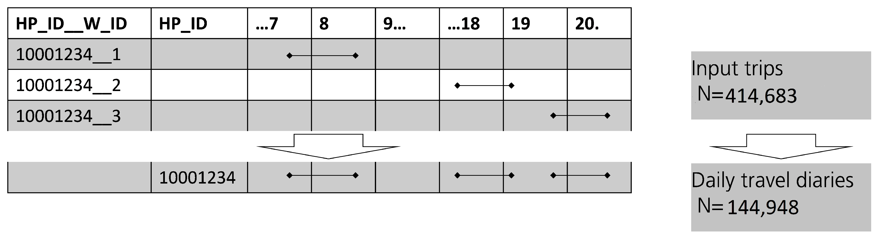
Merging individual trips to daily travel diaries In the next step, the dataset is merged as shown in Figure A1. Thereby, individual trips of the same household and person are merged together to one travel diary with its respective unique ID.
Figure A1. Merging of individual trips to travel diaries.
Energies 14 04349 g0a1
The daily trip diary now has 105,453 observations with the access to all geographical, temporal, technical and socio-economic information from the person and household data set through merging by the identifier. For the weekday and the weights, this is done by default in the flexibility estimation for further analysis and scaling. The data set is then written in a .csv-file as an input into VencoPy:
The MiD2017 B2 trip data set contains a variable zweck, German for ‘purpose’, that differentiates the following trip purposes as shown in Table A4.
Table A4. Trip purpose descriptions in the data set MiD2017 and respective mappings to VencoPy internal trip categories.
Variable ValueGerman DescriptionEnglish DescriptionAggregated Identifier
1Erreichen des ArbeitsplatzesReaching workWORK
2dienstlich/geschäftlichWork tripWORK
3Erreichen dAusbildungsstätte/SchuleReaching educational facilitySCHOOL
4EinkaufShoppingSHOPPING
5private ErledigungPrivate errandSHOPPING
6Bringen/Holen/Begleiten von PersonenBringing, fetching and accompanying personsLEISURE
7FreizeitaktivitätLeisureLEISURE
8nach HauseTrip homeHOME
9Rückweg vom vorherigen WegTrip back from trip beforeHOME
10anderer ZweckOther purposeOTHER
99keine AngabeNot availableNA
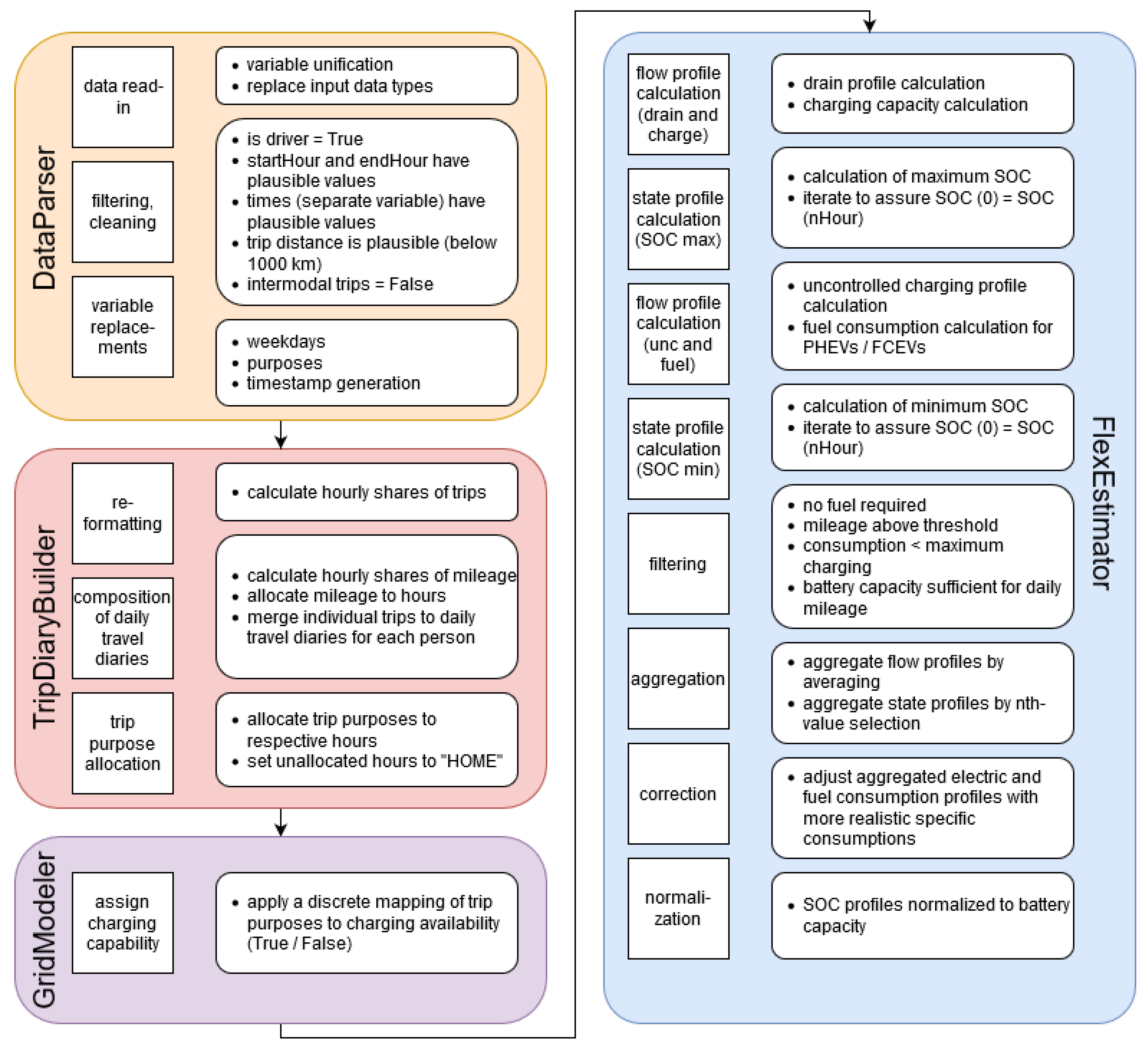
From the trip purposes we are able to learn the location category of a vehicle during the course of the day. This information can, together with assumptions of location-specific charging infrastructure distribution, yield the information whether a charging station is available or not at a respective location category e.g., HOME. We introduce an additional purpose ‘DRIVING’ to account for hours where vehicle holders are mainly driving and thus cannot charge. The filling of trip purposes follows these steps
  • Take the trip distance diary data set and replace all non-zero entries with ‘DRIVING’.
  • We are foremost interested in setting inter-trip hours to specific purposes, and thus we have to go through each diary ID but also through each trip of the diary in its original data set (W_ID) in order to extract and correctly allocate the purpose.
  • All trips are assumed to start at HOME; thus, for the first trip, the hours from beginning to the hour of the trip are filled with ‘HOME’. If the trip starts in the first half of an hour, that hour is not filled with ‘HOME’; if it starts in the second half, it is. If it starts exactly at HH:30, this hour is set to ‘DRIVING’.
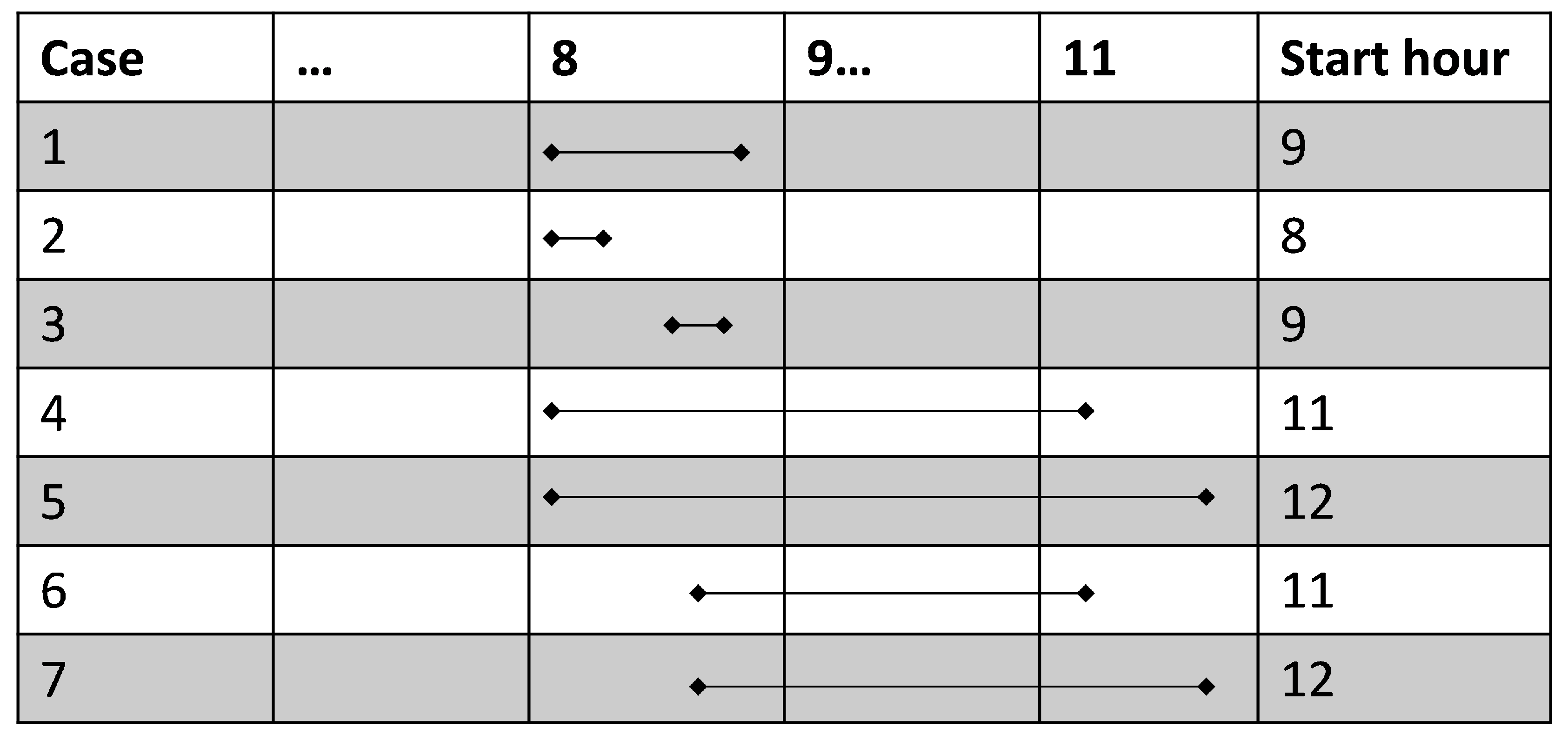
  • For all other trips, the first hour, in which the purpose is not ‘DRIVING’ (or the previous purpose in case of <30 min trips) is identified based on a logical case differentiation schematically shown in the following Figure A2.
Figure A2. Differentiation of cases for the allocation of location purposes based on the trip purpose.
Energies 14 04349 g0a2
Ending hours are currently not differentiated in detail. Thus, the starting hour of the next trip is always determined by the duration of the next trip and the purpose between the two trips ends in the hours before the next trip starts regardless of the start being in the first or second half of the hour, e.g., someone drives to work from 7:30 to 8:20 and then home from 17:20 to 18:10, and thus hour 7 will be determined as ‘DRIVING’; the hours 8–16 will be determined as ‘WORK’, hour 17 as ‘DRIVING’ and the hours from 18 onward will be determined ‘HOME’.

References

  1. Babrowski, S.; Heinrichs, H.; Jochem, P.; Fichtner, W. Load shift potential of electric vehicles in Europe. J. Power Sources 2014, 255, 283–293. [Google Scholar] [CrossRef] [Green Version]
  2. Ried, S.; Dengiz, T.; Soldner, S.; Jochem, P. Aggregating load shifting potentials of electric vehicles for energz system models. In Proceedings of the Institute of Electrical and Electronics Engineers (IEEE) 17th International Conference on the European Energy Market, EEM, Stockholm, Sweden, 16–18 September 2020; Art.Nr. 9221974. Available online: https://ieeexplore.ieee.org/document/9221974 (accessed on 20 May 2021).
  3. Luca de Tena, D. Large Scale Renewable Power Integration with Electric Vehicles. In Long Term Analysis for Germany with a Renewable Based Power Supply; University of Stuttgart: Stuttgart, Germany, 2014. [Google Scholar]
  4. Jochem, P.; Szimba, E.; Reuter-Oppermann, M. How many fast charging stations do we need for European highways? Transp. Res. Part D 2019, 73, 120–129. [Google Scholar] [CrossRef]
  5. Wulff, N.; Steck, F.; Gils, H.C.; Hoyer-Klick, C.; Van den Adel, B.; Anderson, J.E. Comparing Power-System and User-Oriented Battery Electric Vehicle Charging Representation and Its Implications on Energy System Modeling. Energies 2020, 13, 1093. [Google Scholar] [CrossRef] [Green Version]
  6. GitHub—RAMP-Project/RAMP-Mobility: A RAMP Application for Generating Bottom-Up Stochastic Electric Vehicles Load Profiles. Available online: https://github.com/RAMP-project/RAMP-mobility (accessed on 23 April 2021).
  7. Mangipinto, A.; Lombardi, F.; Sanvito, F.D.; Quoilin, S.; Pavičević, M.; Colombo, E. RAMP-Mobility: Time series of electric vehicle consumption and charging strategies for all European countries, in preparation. in preparation.
  8. GitLab—DIW EVU/Emobpy/Emobpy. Available online: https://gitlab.com/diw-evu/emobpy/emobpy (accessed on 23 April 2021).
  9. Gaete-Morales, C.; Kramer, H.; Schill, W.P.; Zerrahn, A. An open tool for creating battery-electric vehicle time series from empirical data—Emobpy. Sci. Data 2021, 8, 152. [Google Scholar] [CrossRef] [PubMed]
  10. Fischer, D.; Harbrecht, A.; Surmann, A.; McKenna, R. Electric vehicles’ impacts on residential electric local profiles—A stochastic modelling approach considering socio-economic, behavioural and spatial factors. Appl. Energy 2019, 233–234, 644–658. [Google Scholar] [CrossRef]
  11. Gnann, T.; Klingler, A.-L.; Kühnbach, M. The load shift potential of plug-in electric vehicles with different amounts of charging infrastructure. J. Power Sources 2018, 390, 20–29. [Google Scholar] [CrossRef]
  12. Ried, S. Gesteuertes Laden von Elektrofahrzeugen in Verteilnetzen mit hoher Einspeisung Erneuerbarer Energien. Ein Beitrag zur Kopplung von Elektrizitäts- und Verkehrssektor; Karlsruher Instituts für Technologie (KIT): Karlsruhe, Germany, 2021. [Google Scholar]
  13. Von Bonin, M.; (Fraunhofer IEE, Kassel, Hesse, Germany). Personal communication, 2021.
  14. Babrowski, S.; Jochem, P.; Fichtner, W. Electricity storage systems in the future German energy sector An optimization of the German electricity generation system until 2040 considering grid restrictions. Comput. Oper. Res. 2016, 66, 228–240. [Google Scholar] [CrossRef]
  15. Luca de Tena, D.; Pregger, T. Impact of electric vehicles on a future renewable energy- based power system in Europe with a focus on Germany. Int. J. Energy Res. 2018, 42, 2670–2685. [Google Scholar] [CrossRef]
  16. DLR / GitLab—VencoPy Code Repository. Available online: https://gitlab.com/dlr-ve/vencopy (accessed on 21 May 2021).
  17. Infas, DLR, IVT and Infas 360: Mobilität in Deutschland —MiD. Ergebnisbericht. Available online: http://www.mobilitaet-in-deutschland.de/pdf/MiD2017_Ergebnisbericht.pdf (accessed on 13 April 2021).
  18. Nobis, C.; Kuhnimhof, T.; Follmer, R.; Bäumer, M. Mobilität in Deutschland—Zeitreihenbericht 2002–2008–2017. Study by infas, DLR, IVT und infas 360 on behalf of the German Minister for Transportation and Digital Infrastructure (FE-Nr. 70.904/15). Bonn, Berlin. Available online: http://www.mobilitaet-in-deutschland.de/pdf/MiD2017_Zeitreihenbericht_2002_2008_2017.pdf (accessed on 23 April 2021).
  19. Howells, M.; Rogner, H.; Strachan, N.; Heaps, C.; Huntington, H.; Kypreos, S.; Hughes, A.; Silveira, S.; DeCarolis, J.; Bazillian, M.; et al. OSeMOSYS: The Open Source Energy Modeling System. An introduction to its ethos, structure and development. Energy Policy 2011, 39, 5850–5870. [Google Scholar] [CrossRef]
  20. Infas, DLR, IVT and Infas 360: Mobilität in Deutschland—MiD. Ergebnisbericht. Struktur—Aufkommen—Emissionen—Trends. Available online: http://www.mobilitaet-in-deutschland.de/pdf/infas_MiD2008_Abschlussbericht_I.pdf (accessed on 21 May 2021).
  21. Nobis, C.; Köhler, K.; Mobilität in Deutschland—MiD Nutzerhandbuch. Study by Infas, DLR, IVT und infas 360 on behalf of the German Minister for Transportation and Digital Infrastructure (FE-Nr. 70.904/15). Bonn, Berlin. Available online: http://www.mobilitaet-in-deutschland.de/pdf/MiD2017_Nutzerhandbuch.pdf (accessed on 23 April 2021).
  22. Eggs, J.; Follmer, R.; Gruschwitz, D.; Nobis, C.; Bäumer, M.; Pfeiffer, M. Mobilität in Deutschland—MiD Methodenbericht. Study by Infas, DLR, IVT und Infas 360 on behalf of the German Minister for Transportation and Digital Infrastructure (FE-Nr. 70.904/15). Bonn, Berlin. Available online: http://www.mobilitaet-in-deutschland.de/pdf/MiD2017_Methodenbericht.pdf (accessed on 23 April 2021).
  23. Heinz, D. Erstellung und Auswertung Repräsentativer Mobilitäts- und Ladeprofile für Elektrofahrzeuge in Deutschland. Bachelor of Science, Karlsruhe Institute of Technology, 16.04.2018. Available online: https://publikationen.bibliothek.kit.edu/1000086372/18281493 (accessed on 17 May 2021).
  24. Schaeuble, J.; Kaschub, T.; Ensslen, A.; Jochem, P.; Fichtner, W. Generating electric vehicle load profiles from empirical data of three EV fleets in Southwest Germany. J. Clean. Prod. 2017, 150, 253–266. [Google Scholar] [CrossRef] [Green Version]
  25. Flammini, M.G.; Prettico, G.; Julea, A.; Fulli, G.; Mazza, A.; Chicco, G. Statistical characterisation of the real transaction data gathered from electric vehicle charging stations. Electr. Power Syst. Res. 2019, 166, 136–150. [Google Scholar] [CrossRef]
Figure 1. Schematic overview of VencoPy workflow components.
Energies 14 04349 g001
Figure 2. Results of the mobility pattern analysis for a representative week based on the sample populations of MiD08 and MiD2017. Figure (a) shows the absolute sample population while the bottom shows the average hourly trip distance. The mean for Figure (b) is calculated by the simple arithmetic mean (‘_mean’) and taking into account MiD trip weights (‘_wMean’).
Energies 14 04349 g002
Figure 3. Weighted average grid connection for electric vehicle fleet differentiated by weekdays.
Energies 14 04349 g003
Figure 4. Weighted average electricity consumption for driving differentiated by weekday.
Energies 14 04349 g004
Figure 5. Weighted average uncontrolled charging in kW. Home charging with a capacity of 11 kW is assumed.
Energies 14 04349 g005
Figure 6. SoC min and max profiles of MiD08 and MiD17. Profiles are based on single-day min and max profile calculation and merged for this plot. For details, see Section 2.1.4. A 50 kWh battery is assumed for this case study.
Energies 14 04349 g006
Table 1. Independent variables and respective algebraic descriptors.
NameElement SymbolSet SymbolDescription
TimetTTime step (t) and temporal scope (T)
VehiclevVVehicle identifier (v) and set of all vehicles (V)
Table 2. Technical assumptions for a VencoPy run.
NameSymbolUnitDescription
Battery capacity C bat kWh The battery capacity of a single vehicle in the respective size and propulsion technology class
Battery security margin minimum m a r g min %Technical exclusion of battery capacity at its minimum for driving
Battery security margin maximum m a r g max %Technical exclusion of battery capacity at its maximum for driving
Specific electricity consumption c o n s elec kWh 100 km Electric consumption of vehicle class
Specific fuel consumption c o n s fuel l 100 km Fuel consumption of vehicle class
Rated power of charging column p charge kW Assumed rated power of each individual vehicle’s grid connection for charging
Table 3. Intermediary profiles of VencoPy.
NameSymbolUnitDescription
Battery drain d r a i n elec ( v , t ) kWh The electricity that flows out of the vehicle battery each hour for driving
Charging capacity p charge , max ( v , t ) kWh Maximum electricity available for charging in each hour
Minimum SoC S o C min ( v , t ) kWh Lower limit for the battery SoC
Maximum SoC S o C max ( v , t ) kWh Upper limit for the battery SoC
Uncontrolled charging c h a r g e unc ( v , t ) kWh Electricity flow from grid to vehicle when no control is exerted
Fuel consumption d r a i n fuel ( v , t ) kWh Fuel consumption of vehicle
Table 4. Aggregate mobility metrics of the original datasets (only motorized trips) and the filtered samples.
Mobility MetricUnitMiD08MiD17Filtered Sample MiD08Filtered Sample MiD17
Mobility quota%9085--
Sample size (trip)1193,290960,619152,621414,683
Number of trips trips mobile person × day 3.83.73.42.9
Daily travel distance km mobile person × day 44463248.5
Daily travel time hh : mm mobile person × day 1:281:341:221:10
Average trip distance km trip 11.5129.417
Total number of trips Mio . trips day 281257120 *111 *
Total distance travelled bn . person km day 3.0803.2141761 *1754 *
* Values taken from [17,18].
Table 5. Literature studies calculating electric vehicle fleet profiles and respective assumptions taken.
ReferenceBattery CapacityElectric ConsumptionGrid ModelingAvailable Profiles
[23]multiple 1multiple 1multiple 2 c h a r g e unc , p charge , max , d r a i n elec
[12] 70 kWh veh 16 kWh 100 km 9.1 kW for home charging c h a r g e unc
[24]multiple 3multiple 3multiple 3 c h a r g e unc
Case study 50 kWh veh 20 kWh 100 km 11 kW c h a r g e unc , p charge , max , d r a i n elec
1 22 values for 13 different segments. 2 3.7 kW for work, education and home charging, 22 kW for shopping and leisure. 3 Vehicle models see [24], charging up to 22 kW stations.
Publisher’s Note: MDPI stays neutral with regard to jurisdictional claims in published maps and institutional affiliations.

