Steam Turbine Rotor Stress Control through Nonlinear Model Predictive Control

Abstract

The current flexibility of the energy market requires operating steam turbines that have challenging operation requirements such as variable steam conditions and higher number of startups. This article proposes an advanced control system based on the Nonlinear Model Predictive Control (NMPC) technique, which allows to speed up the start-up of steam turbines and increase the energy produced while maintaining rotor stress as a constraint variable. A soft sensor for the online calculation of rotor stress is presented together with the steam turbine control logic. Then, we present how the computational cost of the controller was contained by reducing the order of the formulation of the optimization problem, adjusting the scheduling of the optimizer routine, and tuning the parameters of the controller itself. The performance of the control system has been compared with respect to the PI Controller architecture fed by the soft sensor results and with standard pre-calculated curves. The control architecture was evaluated in a simulation exploiting actual data from a Concentrated Solar Power Plant. The NMPC technique shows an increase in performance, with respect to the custom PI control application, and encouraging results.

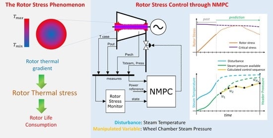
1. Introduction

In the current energy market, renewable sources and flexible power plants are increasingly exploited in order to meet the energy demand of increasingly connected cities [1], where smart grids are going to become a consolidated reality [2,3]. In this context, the design of new power plants must aim at increasing the level of flexibility, with a resulting multitude of challenges in terms of degradation of the components, restrictions related to the environmental impact, and required level of workforce specialization. For these reasons, the design of Steam Turbines (STs) nowadays must take into account frequent discontinuous operations. For instance, in the case of Concentrated Solar Power Plants (CSPP), the inlet steam highly depends on the weather conditions [4], while in industrial power generation, the discontinuity is related to the scheduling of the electricity production, optimized according to the prices of energy media (natural gas and electricity) that vary on an hourly or daily basis. One of the most important aspects related to discontinuous operation is the need to enforce protection against stress induced by thermal transients, which, due to the continuous changes in the steam conditions, can lead to faster aging of the turbine and, in extreme cases, to component failure due to nucleation and propagation of cracks. While almost every ST component is affected by thermal stress aging, transient thermal stresses in rotors often represent the factor determining the minimum allowable start-up time and the maximum allowable production during start-up. The start-up optimization is carried out through several different steps. The first one usually takes place during the design phase of the machine itself, e.g., through a proper design of the rotor critical locations, which are mostly affected by peak stress. During the design phase, load curves are also optimized by exploiting accurate process models evaluating the specific plant components to which they are connected. The last phase for the start-up design and optimization is represented by the control logic design, which is typically implemented through Proportional Integral Derivative (PID) controllers. In more advanced control systems, which are described later on, the control approaches are based on predictive methodologies considering the machine thermal dynamics or on particular heuristics.

Thermal stress phenomena have been extensively studied in literature, mostly by focusing on their effects and on measurement procedures for early identification of aging phenomena. These are of crucial importance especially for critical components, such as rotors, where cracks after nucleation can rapidly propagate due to vibration phenomena that in normal conditions do not affect rotor integrity. In addition, low cycle fatigue damage cannot be directly detected with non-destructive methodologies. Indirect measurements of the most severe effects of thermal stress are often associated with vibrational phenomena on the machine axis. Most often, the effects of excessive machine stress can only be verified after dismantling the machine. Non-destructive tests are not always capable to highlight issues on the rotor and often cracks can be found only after the rotor is taken out of service.

The management of the machine thermal stress is a rather complex operation and, from the control point of view, is faced through a sequence of steps. In more recent years, these operations have been automated, thanks to a wider use of sensors, which have led to in-depth studies of their behavior through increasingly reliable models. An example of automated pre-warm is described by Badami et al. [5], in which a fuzzy logic-based supervisor has been designed to speed up the rotor warming phase, while taking into account the rotor stress conditions before the cold start of the machine.

The literature highlights two main complementary methods for the control of the rotor thermal stress, which concern either the limitation of the inlet steam flow—common in every steam plant—or the regulation of the temperature of the inlet steam, available only in specific plants. In Combined Cycle (CC) systems, the outlet steam temperature of the Heat Recovery Steam Generator (HRSG) can be adjusted by the direct control of the gas generator. However, this kind of operation shows the disadvantage of forcing the gas turbine to lower efficiency operating conditions. De-superheating of inlet steam by attemperators is also a possible solution for limiting the thermal stress in STs, at the cost of increasing installation costs. For these reasons, a common control strategy aims at adjusting the Heat Transfer Coefficient (HTC) or the inlet steam mass flow. As a first approximation, we can divide the work related to the start-up control into three categories: The first one refers to the modeling of the thermal behavior of the machines and/or connected systems, the second one is linked to the offline calculation of turbomachinery and related system load curves, while the third one concerns the startup online control with/without thermal stress related logic.

Some examples of works related to modelling topics are presented by Carnero et al. [6], which introduce a soft-sensor application aimed at monitoring the ST stress, by exploiting heat transfer equation to model the thermal dynamics in the rotor. Sun et al. in their paper [7] present a soft sensor that models the rotor temperature through transfer function and the damage due to thermal stress through polynomials. Rusin et al. [8] propose two modelling methodologies based on Green’s function, Duhamel’s integral and Neural Networks (NN). These approaches can be used to solve the inverse problem aimed at optimizing the operation of steam machines and are also exploited in a similar way by Banaszkiewicz et al. [9,10]. Dominiczak et al. [11] apply NNs for the prediction of temperature and stress in the ST critical points.

Offline optimization approaches have been proposed by Casella et al. for optimizing the load curve of a real CC Power Plant (CCPP) through models developed in Modelica and Dymola [12]. Faille et al. [13] followed a similar approach with the objective of minimizing the start-up time.

A brief review of online control applications aimed at speeding up the startup of STs show three main classes of methodologies: (i) PID controllers, (ii) Artificial Intelligence (AI)-based techniques, and (iii) Model Predictive Control (MPC). Sun et al. [14] present a controller based on polynomials and PID aimed at extending the life of the machine, limiting its cumulative damage. Boulos et al. [15] propose three different control methods based on pure PID controller, Fuzzy-PID, and a Fuzzy Logic controller, applied to the startup of a CCPP by acting on the load rate. Matsumoto et al. [16] introduce a complex system based Fuzzy Logic and NNs to control the schedule of the power plant load curve as a function of the current status of the machines and the HRSG. MPC architectures have been widely studied for startup applications. Excellent examples are proposed by Nakai et al. [17], who describe a MPC based on linear programming and models based on heat conduction equations. Gallestey et al. [18] present a linear MPC strategy that integrates Fatigue Crack-Growth Models to the aim of extending the residual lifetime of the machine with consequent relevant economic benefits for a power plant application. Shirakawa et al. [19] describe a multi-objective MPC, which integrates several components of a power plant of 600 MW by including the thermal dynamics of the involved STs and by exploiting a complex system of NN models and thermal equations as well as a Genetic Algorithm (GA) for optimization. Larsson et al. extend the MPC application by using different nonlinear components models of a CCPP [20], with a simulation approach implemented in Modelica. D’Amato et al. [21,22], present several excellent works, in which MPC is applied to the startup of turbomachines, by exploiting heat equations and linearization procedures to implement an MPC strategy in Programmable Logic Controllers (PLCs). Rua et al. compared a linear and a nonlinear formulation of MPC to optimize the startup of a combined cycle while taking into account stress limits on the walls of the high-pressure steam drum and the steam turbine rotor [23].

Once the turbine has been correctly started, the management of the variability of the inlet steam conditions and the tracking of the power setpoint are often performed through PI control techniques, fuzzy PID [24], robust control [25], and in some cases through MPC techniques [26].

An in-depth analysis of the aforementioned works shows two possible methodologies for implementing an effective control system for the ST startup, PID controllers and MPCs. The former ones ensure good performance and usually lower modeling and implementation efforts, with some shortcomings related to the inability of the PID controllers to anticipate any control actions to avoid stress overshoots and problematic operating points. On the other hand, the MPC-based strategies naturally manage all the constraints of the machine and, thanks to the model-based approach, can predict its dynamic behavior. This capability makes the control actions effective by allowing anticipation and avoidance of numerous undesired phenomena. Although MPC appears the best-performing strategy, it shows some heavy limitations related to the online calculation of the control action, which requires calculation times that are often not compatible with PLC platforms.

The present research work is part of this context, as it aims at identifying and overcoming the most relevant bottlenecks in the application of MPC for controlling the ST power startup through a local point of view of the phenomenon of the thermal transient, in which the controller focuses on the steam turbine. In particular, this article presents a Nonlinear MPC (NMPC), which aims at maximizing the energy produced during the power startup of STs, by integrating a series of nonlinear models that describe the temperature dynamics in different sections of the rotor as well as the thermodynamic and mechanical behavior of the machine. The modelling scheme implements hybrid methods based on heat equations and empirical numerical models for predicting specific internal quantities. The NMPC optimizes the power load curve during the startup, through a tracking formulation of the optimization strategy, in which the maximum power reference is received from the Distributed Control System (DCS) of the plant. In particular, this article presents several novelties. In the first place, it compares the standard baseline curves for steam turbine start-up with the application of a PI architecture including the soft sensor calculating the rotor stress. Later this PI architecture is compared with the NLMPC application showing the benefits of this control procedure. It also has to be remarked that while other works aim at the application of MPC strategies to the whole plant, here the focus lies on the control of the single steam turbine. The application of these procedures to a CSP case through real data is of particular interest.

The paper is organized as follows. Section 2 describes the modeling methodologies and validation procedures for the models obtained. Section 3 provides a brief introduction on PID and NMPC control and describes the structure of each implemented controller and the associated technical solutions. Section 4 discusses the results of the simulation studies for the implemented controllers by comparing their performances and providing guidelines for tuning the NMPC control parameters. Section 5 provide final comments to the obtained results and some concluding remarks.

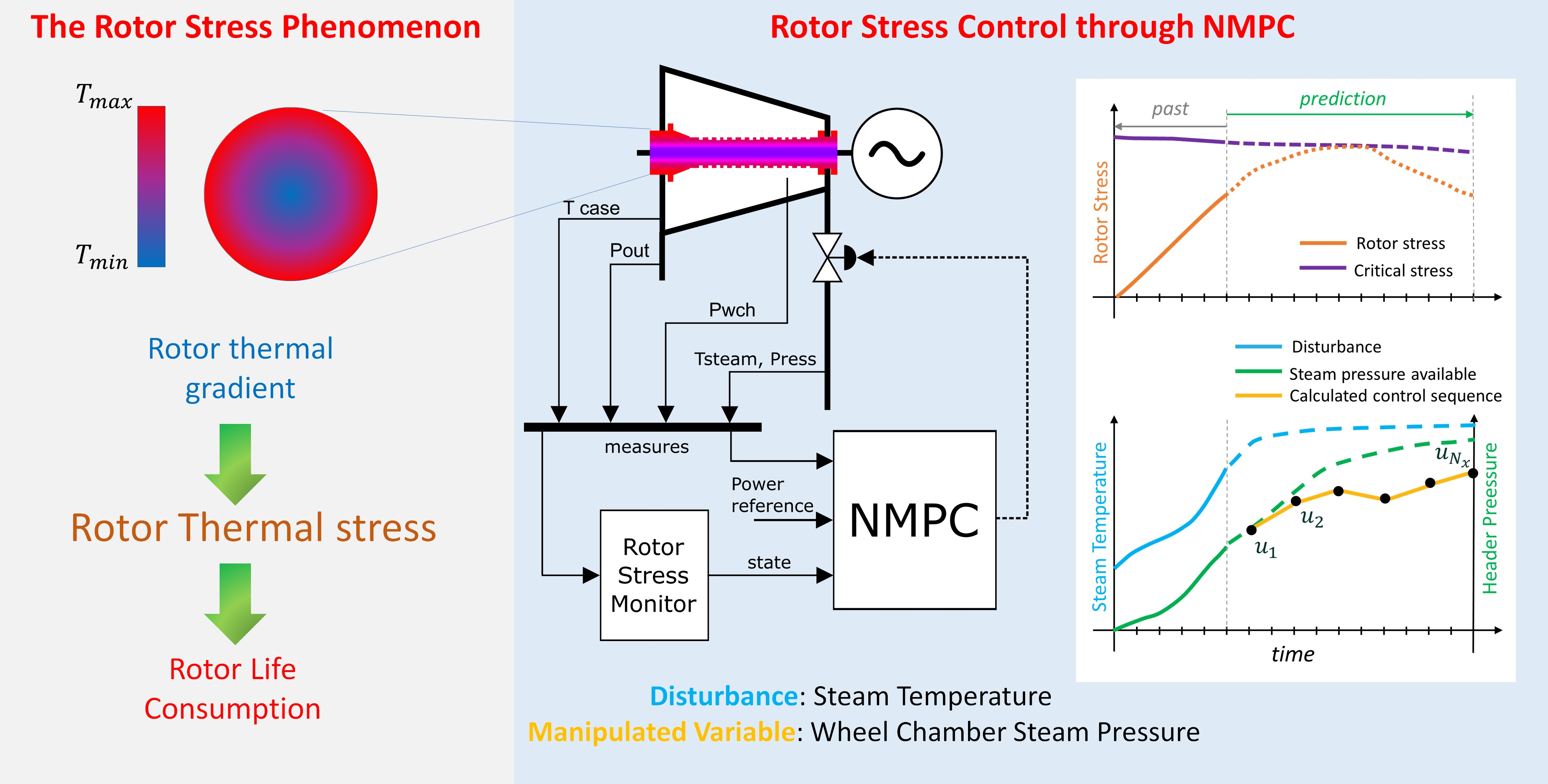
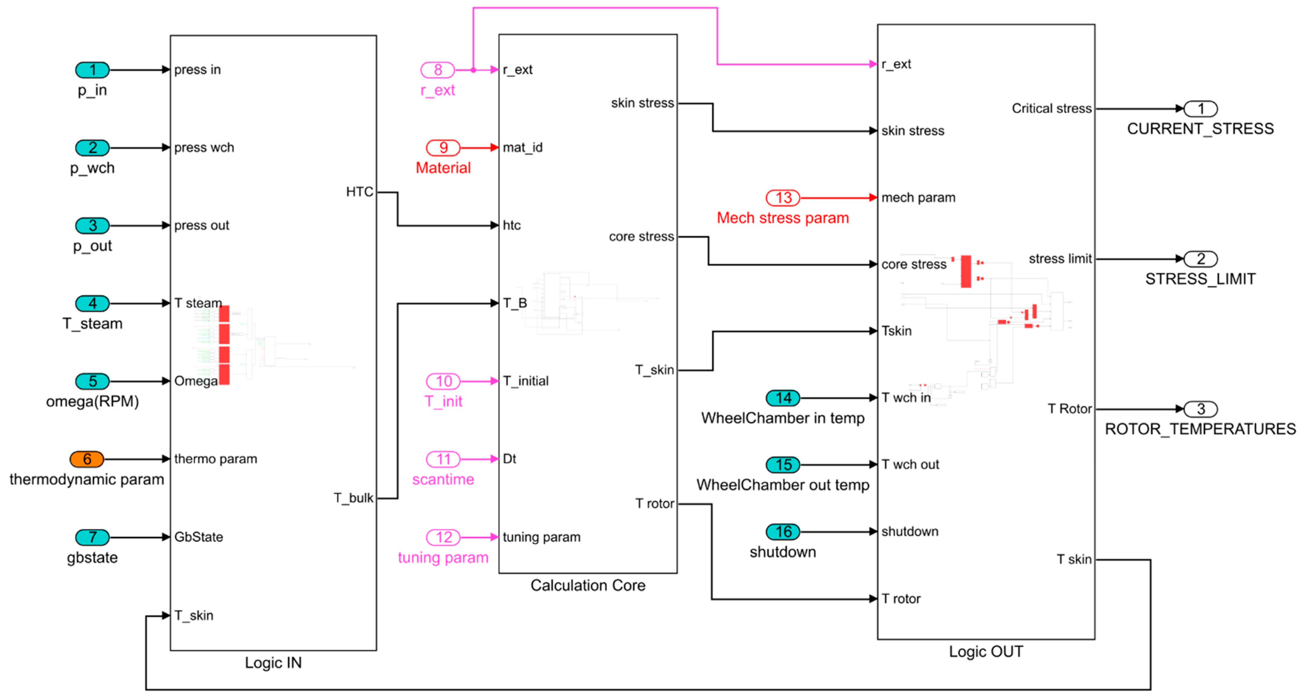
2. Steam Turbine Modelling Approach and Rotor Stress Monitoring

The first fundamental step to define an effective control strategy for optimizing the ST start-up is to design a tool capable of monitoring the thermal state of the machine. As previously mentioned, the stress can only be measured using particularly invasive hardware measuring instruments, which must be designed to work at rather high temperatures and pressures, with all the consequent technical difficulties (e.g., pyrometers, which also require a temperature/stress conversion system while strain gauges are usually unsuitable for rotating equipment). These issues have been overcome through an approach called “soft-sensing”, which allows extrapolating, through suitable algorithms, detailed information from the sensors that are normally installed on the machine. This section describes an instrument called the Rotor Stress Monitor (RSM) [27], depicted in Figure 1, which is used to this purpose and whose calculation steps are described in detail in the next sections.

The RSM algorithm allows calculating the current stress, its current limit, and the temperatures of the rotor based on:

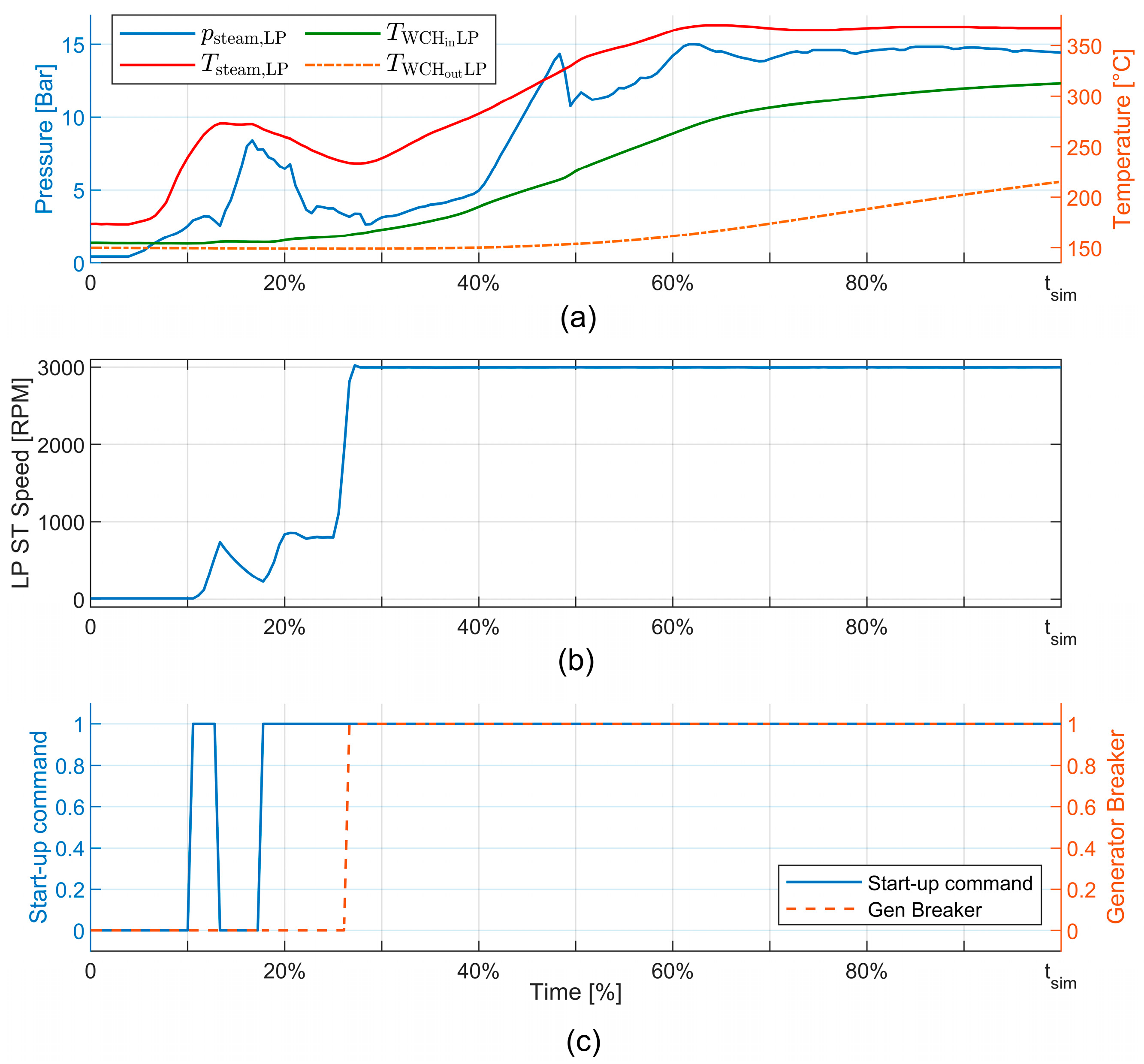
• The state of the generator breaker that connects the electric generator to the network;
• The state of the ST startup;
• The rotor speed;
• The inlet, outlet, and wheel chamber pressures;
• The temperature of the steam in the inlet;
• The ST casing temperature;
• Some parameters describing the dependence of the rotor temperature on material properties, limits on pressures, temperatures, speeds, and coefficients to calibrate stress values.

The Reduced Order Model (ROM), at the core of this soft sensor, despite its limited computational cost, is suitable to develop the MPC strategies. The description of the model features is organized into threes subsections focused on:

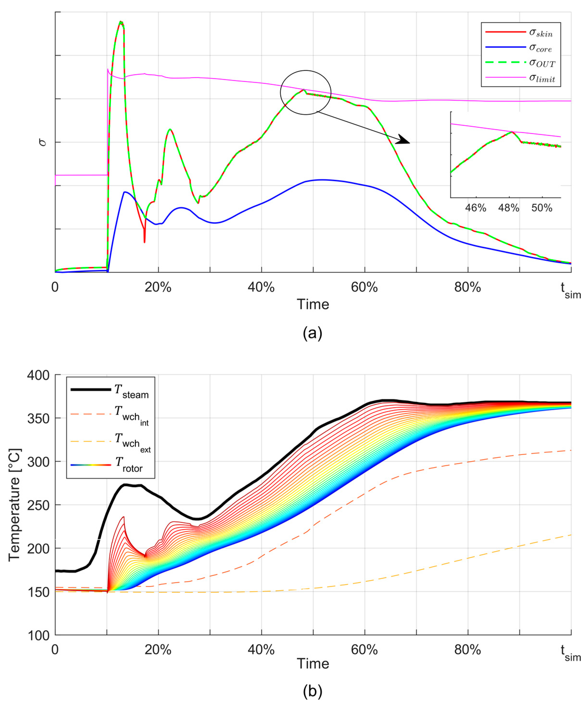
• Calculation of rotor temperature;
• Calculation of rotor thermal stress;
• Derivation of boundary conditions for the thermal model.

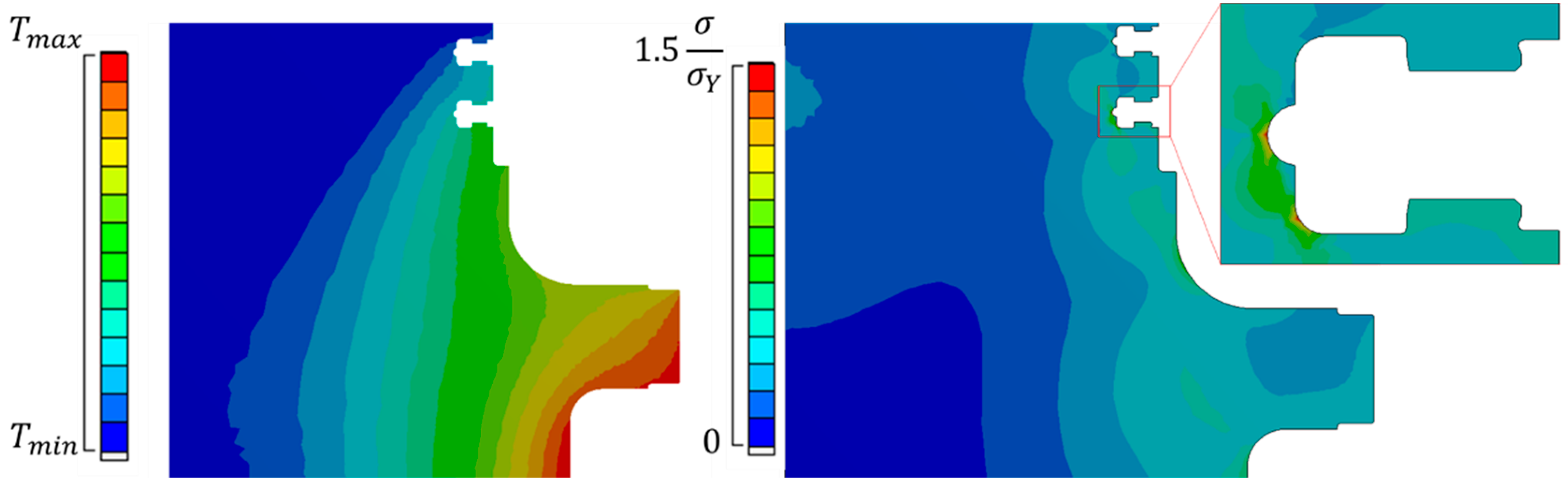
2.1. Thermal Model

In order to correctly evaluate thermal stresses, the model must satisfy the minimum requirements in terms of accuracy. However, it is also extremely important for the model to take into account maximum computational cost requirements set by common control industrial hardware e.g., PLCs. Therefore, standard detailed calculation procedures (such as the one used during rotor design phase) based on the 2D and 3D Finite Element Model (FEM) implementing rotor detailed geometrical description are not suitable for control purposes. Such models, which are used to explore the effect of complex thermal transient scenarios, must be simplified into Reduced Order Models (ROM).

In the present case, the selected approach is based on the assumption that the rotor geometry can be approximated through a cylindrical axisymmetric model so that the thermal model can be described (in cylindrical coordinates) by the following partial differential equation:

$$\rho c_p\frac{\partial T}{\partial t}=\frac{1}{r}\frac{\partial }{\partial r}\left(kr\frac{\partial T}{\partial r}\right)$$

(1)

Subjected to the following boundary conditions:

$$\{\begin{array}{c}{\frac{\partial T}{\partial r}|}_{r=0}=0\\ -k{\frac{\partial T}{\partial r}|}_{r=R_{ext}}=HTC\left(t\right)\cdot \left[T{|}_{R=R_{ext}}-T_{bulk}\left(t\right)\right]\end{array}$$

(2)

where $T$ is the rotor temperature, function of radius $r$ and time $t$, $HTC\left(t\right)$ is the HTC as a function of time, $T_{bulk}$ is the steam temperature, $\rho$ is the rotor density, $C_p$ is the rotor local heat capacity (function of temperature), and K is the rotor local thermal conductivity (function of temperature). It can be observed that:

• The main assumption is that the rotor geometry can be described by an infinitely extended cylinder excluding the dependency from the axial coordinate;
• Local variations of material properties are taken into account leading to a non-linear heat transfer equation with a non-homogeneous material;
• Since HTC and $T_{bulk}$ are time-dependent the model is suitable to complex heat transient scenarios.

For the solution of the problem, an explicit finite difference scheme (backward Euler) has been selected with $N$ radial locations and a spatial discretization of $\mathsf{\Delta }r=r_{i+1}-r_i$. As a consequence:

$$T_j^{\left(i+1\right)}=f\left(T_j^{\left(i\right)},T_{j-1}^{\left(i\right)},T_{j+1}^{\left(i\right)},\dots \right)$$

(3)

As well known the stability of this numerical scheme depends on the selected time discretization $\mathsf{\Delta }t$. Partial derivatives in space and time are discretized as follows:

$$\frac{\partial T}{\partial t}=\frac{T_j^{\left(i+1\right)}-T_j^{\left(i\right)}}{\mathsf{\Delta }t}$$

(4)

$$\frac{\partial T}{\partial r}=\frac{T_{j+1}^{\left(i\right)}-T_j^{\left(i\right)}}{\mathsf{\Delta }r}$$

(5)

The choice of an explicit method is driven by the fact that in this way, a non-linear solver is not necessary to evaluate rotor radial temperature distribution from step to step. In any case, this poses a limit on the maximum allowable timestep length that has been explored considering the thermal diffusivity of the material of interest for this kind of analysis. In addition, the limit to the timestep length poses challenges for the development of the control scheme (which are later explained). Noticeably, after numerical discretization, the nonlinear partial differential equation can be reconducted to a general control scheme:

$$T^{\left(j+1\right)}=A^{\left(j\right)}\cdot T^{\left(j\right)}+B\cdot \phi \left(T_N^{\left(j\right)},HT{C}^{\left(j\right)},T_{bulk}^{\left(j\right)}\right)$$

(6)

$A^{\left(j\right)}\in R^{n\times n}$ is a tri-diagonal matrix wherein the non-zero elements are expressed as follows:

$$a_{i,i}^{\left(j\right)}=1-\frac{\mathsf{\Delta }t}{{(\mathsf{\Delta }r)}^2}{\alpha }_{i-\frac{1}{2}}^{\left(j\right)}\left(1-\frac{\mathsf{\Delta }r}{2r_i}\right)-\frac{\mathsf{\Delta }t}{{(\mathsf{\Delta }r)}^2}{\alpha }_{i+\frac{1}{2}}^{\left(j\right)}\left(1+\frac{\mathsf{\Delta }r}{2r_i}\right)$$

(7)

$$a_{i-1,i}^{\left(j\right)}=\frac{\mathsf{\Delta }t}{{(\mathsf{\Delta }r)}^2}{\alpha }_{i-\frac{1}{2}}^{\left(j\right)}\left(1-\frac{\mathsf{\Delta }r}{2r_i}\right)$$

(8)

$$a_{i+1,i}^{\left(j\right)}=\frac{\mathsf{\Delta }t}{{(\mathsf{\Delta }r)}^2}{\alpha }_{i+\frac{1}{2}}^{\left(j\right)}\left(1-\frac{\mathsf{\Delta }r}{2r_i}\right)$$

(9)

where ${\alpha }^{\left(j\right)}=\frac{k^{\left(j\right)}}{\left({\rho }^j\cdot c_p^{\left(j\right)}\right)}$ is the thermal diffusivity evaluated at the node $j$. $\phi$ is the heat flow transferred by convection to the cylinder:

$$\phi =a_{N+1}^{\left(j\right)}\cdot HT{C}^{\left(j\right)}\frac{2\mathsf{\Delta }r}{k_{\left(T=T_N^{\left(j\right)}\right)}}\left(T_{bulk}^{\left(j\right)}-T_N^{\left(j\right)}\right)$$

(10)

The previous expressions highlight a linear dependence of the cylinder temperature state on the heat flow (such as also highlighted by Nakai et al. [17]). The creation of a purely linear control system based on this model is basically compromised by the fact that heat flow is a non-linear combination of disturbance (bulk temperature), system state (last node temperature), and control (HTC). In addition, as the rotor surface temperature approaches bulk temperature, the effect of a control action on HTC becomes less relevant.

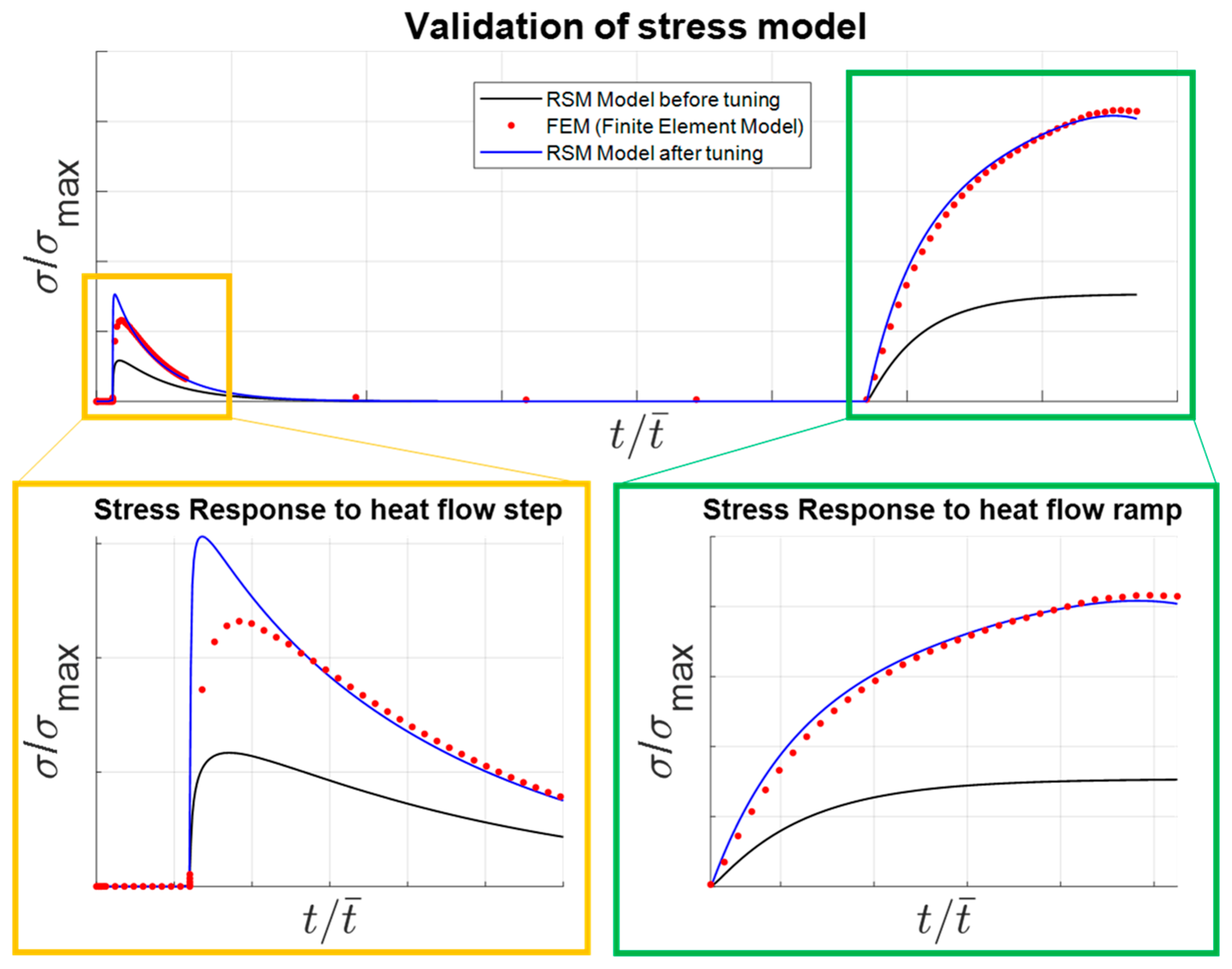
2.2. Rotor Stress Models

The temperature field can be exploited to obtain the cylinder stress approximating the actual rotor stress. For this specific case, a generalized plane strain assumption is suitable, leading to the following expression for the Von Mises stress ${\sigma }_{eqv}$ as a function of temperature $T\left(r\right)$:

$${\sigma }_{eqv}=|\frac{\beta E}{1-\upsilon }\left(T\left(R\right)-\frac{2}{R^2}{{\displaystyle \int }}_0^{R}Trdr\right)|$$

(11)

where $\beta$ is the thermal expansion coefficient, $E$ is the Young modulus, and $\nu$ is the Poisson ratio.

Equation (11) provides an estimate of the equivalent stress on the cylinder external surface and is suitable for the identification of crack nucleation (a similar expression can be obtained also for rotor core stress and can be used for detecting crack nucleation and propagation). The effect of centrifugal stress is not taken into account here, as it does not depend on the temperature field, but can be included in an additional term for control purposes.

The stress integral expression can be numerically approximated according to the following linear relation:

$${\sigma }_{eqv}=C\cdot T={\left[\begin{array}{cccc}{c}_1& c_2& \dots & c_n\end{array}\right]}^T\cdot \left[\begin{array}{cccc}{T}_1& T_2& \dots & T_n\end{array}\right]$$

(12)

where:

$$C=\frac{\beta E}{1-\upsilon }\left[\begin{array}{cccc}-\frac{{\left(\mathsf{\Delta }r\right)}^2}{R^2}& -\frac{2r_2\mathsf{\Delta }r}{R^2}& \dots & \begin{array}{cc}-\frac{2r_{N-1}\mathsf{\Delta }r}{R^2}& 1-\frac{\mathsf{\Delta }r}{R}\end{array}\end{array}\right]$$

(13)

Moreover, the maximum allowable stress for the rotor can be expressed as a function of the local cylinder temperature in order to take into account the typical degradation of steel strength with temperature. Usually, a polynomial approximation is suitable for this purpose. In addition, the coefficients of the polynomial can be updated from start to start in accordance with the expected start-up severity and frequency (for instance, in CSP applications the cold start-up, being the most severe and also less frequent, is usually set up with a high maximum allowable stress limit).

In any case, an actual rotor geometry holds different critical locations, unlike the considered cylinder model, where stress values are amplified. Amplification factors for stress need to be calculated through a dedicated 2D thermo-mechanical Finite Element Analysis (FEA). These factors can be used to properly tune and align the results of the simplified cylindrical model to those of a real rotor geometry (examples of this kind of procedure are given for example in [9,28]). Typically, critical rotor locations are represented by fillets in the proximity of the first stage and bucket tail grooves, where differential expansion drives complex stress conditions and even local plasticization. An example is shown in Figure 2, where the contour plots of Von Mises equivalent stress are shown for an axis-symmetric simulation, at the load step where the stress peak is reached.

Two set of tuning functions are created to enable a good correspondence between Finite Element Models and Rotor Stress Monitor. Many shapes of increasing complexity can be chosen for the tuning functions that adjust the inputs and the outputs of the previously explained Reduced Order Model. The performance of the adjustment procedure on tuning functions can be evaluated by testing campaigns: In other words, collecting the response of the system to a stepwise and/or ramp increase of heat flow is able to give relevant indications on the behavior shown in more complex scenarios. A simple example of the response to a testing mission before and after the tuning procedure is shown in Figure 3, where the stress evaluated by FEA in the most critical location is also plotted. Here it can be seen how the chosen tuning function setup is able to match the stress response to a ramp increase of heat flow within a 5% error. At the same time, we chose to keep a conservative margin (~30%) for the response of the system to a step heat flow increase.

2.3. Power and HTC Calculation

The thermo-mechanical FE transient simulation, used to assess ST components’ reliability and strength, involves, during the pre-processing phase, a detailed calculation of HTCs and bulk temperatures. These calculations take into account the thermodynamic behavior and geometry of the specific ST and, in the most complex scenario, may also involve Computational Fluid Dynamics (CFD) evaluation with all the geometrical details of the specific ST. These kinds of calculations need to be included in a simplified form for rotor stress monitoring and control purposes through simplified thermodynamic transfer functions. Such functions basically summarize the thermodynamic behavior of the turbine and enable the HTCs calculation, bulk temperature, or ST output power for the location where the stress has to be evaluated. The need for simplified calculations lies in the computational constraint of a User Control Panel implementation. Typically, polynomial transfer functions are capable to model, with sufficient precision, the HTCs variation corresponding to the operation field of the rotor. A typical scenario occurs when the influence of controlled and un-controlled extraction can be considered negligible for the determination of the ST condition during start-up, and $HTC$, power $W$, and bulk temperature can be approximated by polynomial functions of ST inlet and outlet pressure, inlet temperature, and wheel chamber pressure (the steam pressure after the group including the control stage and the control valve), as follows:

$$HTC=f\left(P_{\mathrm{in}},P_{\mathrm{wch}},P_{\mathrm{out}},T_{\mathrm{steam}}\right)$$

(14)

$$W=h\left(P_{\mathrm{in}},P_{\mathrm{wch}},P_{\mathrm{out}},T_{\mathrm{steam}}\right)$$

(15)

$$T_{bulk}=T_{\mathrm{B}}\left(P_{\mathrm{in}},P_{\mathrm{wch}},P_{\mathrm{out}},T_{\mathrm{steam}}\right)$$

(16)

3. Rotor Stress Control Strategies

This section focuses on the main aspects of PID and MPC strategies in order to introduce the NMPC approach aimed at optimizing the ST power startup and limiting the related rotor stress.

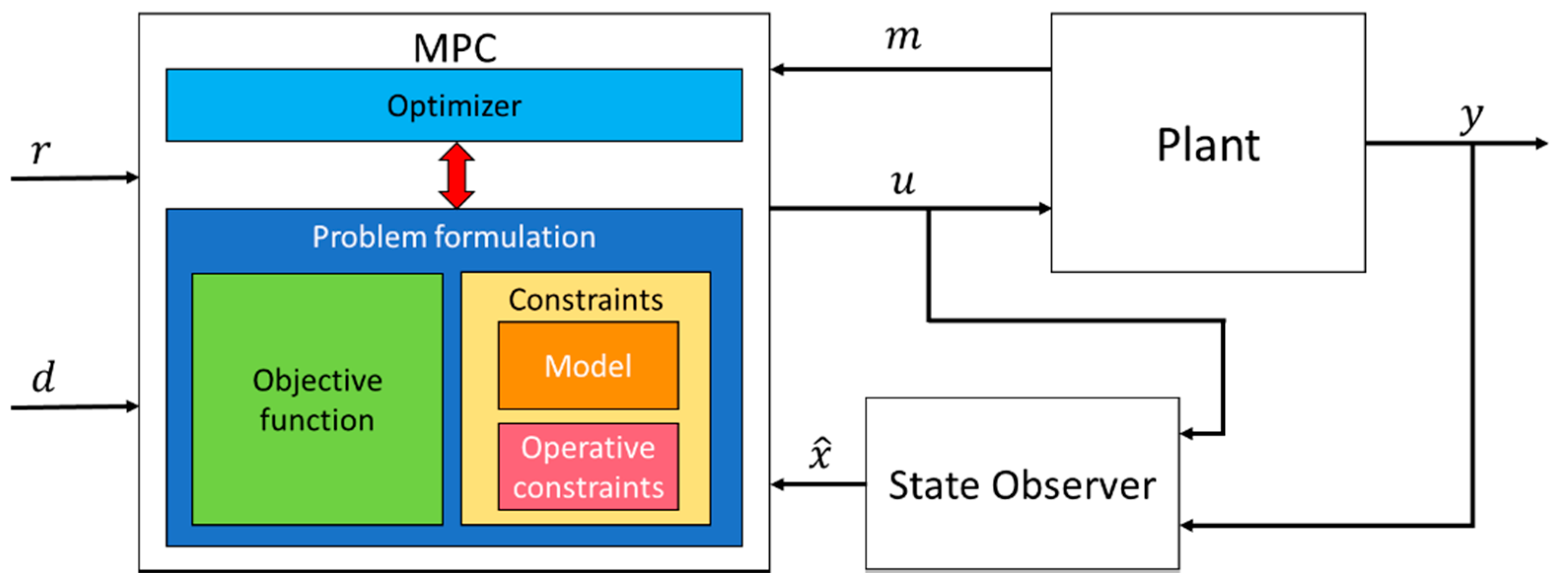
3.1. Background on PI and MPC Control Strategies

The PID controller is the most widespread control algorithm in industry, exploited in more than 90% industrial controllers [29], due to its simple implementation and its effectiveness. Its main characteristic lies in the use of an error-driven philosophy typical of the Model Free control approach [30]. Its implementations may differ depending on the specific application and its realizations have been widely studied in the literature and applied to industrial cases.

The success of PID control strategy is closely linked to factors related to its simplicity as well as to the effectiveness and large availability of efficient and ready-to-use PID controller products. PID is one of the first techniques developed in the field of control engineering, as it was possible to implement it through mechanisms (such as in the case of the Centrifugal governor, the first ST controller that was based on proportional control) or through simple electromechanical circuits and, afterwards, through analog and digital electronics. Its effectiveness also relies on the immediacy of the control action, a necessary feature in the case of low-level control loops (closer to the machines or basic processes such as pressure, flow, level control, etc.). Last but not least is the effectiveness of the control action on processes that work in almost stable operating points, in which the performances achievable through a PID controller are usually quite satisfactory.

The positive aspects of the PID controller are, however, counterbalanced by a series of disadvantages that make it not always the ideal choice for process control. In the first point, PIDs are a Single Input Single Output (SISO) and can act on a single manipulable variable. Multi Input Multi Output (MIMO) control can be obtained through complex control methodologies such as the decoupling of the system dynamics [31] or other more complex logics [32]. However, the most complex aspect, which is widely analyzed in the literature [33], is the tuning of its parameters. The most common approaches are based on standard Ziegler–Nichols (ZN) methods [34], relays [35], and several analytic rules [36]. Auto-tuning methods and approaches based on offline simulation are particularly studied and deepened in literature [37]. Furthermore, AI through Artificial Neural Networks (ANN), Fuzzy Logic, and Evolutionary Algorithms have been widely explored [38].

The MPC is an advanced control technique developed in the refinery and petrochemical industry context in the 1970s, and subsequently deepened in the academic world starting from an initial diffidence and skepticism that allowed, firstly, the definition and stabilization of the theoretical foundations of this methodology and, subsequently, its consistent evolution and research advancement. The foundations of this control technique lie in three basic ideas: (i) The prediction of future behavior of the controlled process, through adequate mathematical models; (ii) the optimization of the control path aimed at minimizing a specific cost function and satisfying process and actuators operative constraints; and (iii) the action on the controlled process through a receding control horizon that implements a closed loop control strategy by manipulating only the current manipulable variable, such as introduced by Propoi [39].

The ideas behind the first applications, based on Dynamic Matrix Control (DMC) [40] and the Identification-Command (IDCOM) software [41], were extended in two fundamental works of Clarke et al. [42,43] and then unified by Garcia et al. in 1989 in their seminal paper [44]. The numerous works in the literature have shown, over time, from an academic point of view, the effectiveness and limitations of this control approach, which is now considered to be the standard for the control of MIMO systems, not only in the industrial context, in which it is obviously widely used [45,46,47,48]. Some novel interesting examples of MPC methodologies application related to the energy management or power generation have been presented by Camacho et al. in their work [49], in which a hybrid NMPC regulates the outlet temperature of a solar collector field in order to optimize the operating condition of a solar cooling plant, by Kong et al. in their article [50] that presents a nonlinear economic MPC approach to maximize the energy produced by wind turbines over all the operating points in variable speed conditions, and by Darwish et al., who presented an integration of Dual-mode MPC and Generalized Predictive Control (GPC) for optimizing the startup of a steam power plant [51].

In deeper detail, the MPC strategy requires three well-defined elements in order to achieve satisfactory control performances:

• A sufficiently accurate process model, i.e., the core of the MPC approach, whose complexity must balance two counteracting issues related to the accuracy of the short-long term dynamic predictions and the computation burden required to simulate it. In the literature, several realizations of the process models are proposed, starting from linear state space models, linear or nonlinear autoregressive exogenous models (ARX) [52], and Hammerstein Wiener models [53], which are considered the standard for industrial process modelling, up to ANNs [54,55], which are less widespread in control applications but particularly effective in modelling nonlinear behavior. Furthermore, the modelling objective it is not only related to the future behavior prediction, but also to the estimation of the current state of the controlled process, which might not be accessible or measurable.
• A cost function describing one or more indexes to be optimized. Such cost function depends on the specific task and in general is related to energy description of the system, economic costs, or particular specific mathematical relationships. From this point of view, the MPC can fundamentally be a single or a multi objective optimization problem.
• A set of constraints aimed at describing the operative boundaries of the system, including the process itself as well as actuators and related subsystems.

The combination of these three elements defines the complexity of the MPC and, consequently, the difficulty in solving the optimization strategy in real-time. The term “linear MPC” is used when the operating models and constraints of the process to be controlled are linear, and when the cost function is linear or quadratic. The term “non-linear MPC” is adopted when one of the first two elements is nonlinear and/or the cost function can be described by a Taylor series of a degree higher than two.

The typical MPC closed loop architecture is depicted in Figure 4, where its different elements are divided in functional blocks: (i) The real controlled process/plant; (ii) the state observer (sometimes included within the MPC); and (iii) the MPC block. More in detail, the MPC block includes a mathematical formulation of the optimization problem, including constraints and process/plant dynamics, an objective function and an optimizer, which includes a set of optimization algorithms and routines tailored for the specific application.

The MPC solves in real-time an optimization problem that in the linear case can be described as:

$$\{\begin{array}{c}\underset{u}{\min }J\left(x_t, N_p,N_c\right)\\ \begin{array}{cc}\hfill x\left(k+1\right)& =Ax\left(k\right)+Bu\left(k\right)\hfill \\ \hfill y\left(k\right)& =Cx\left(k\right)+Du\left(k\right)\hfill \\ \hfill x\left(0\right)& =x_0\hfill \\ \hfill \mathsf{\Delta }u\left(k\right)& =u\left(k\right)-u\left(k-1\right)\hfill \\ \hfill y_{min}& \le y\left(k\right)\le y_{max}\hfill \\ \hfill u_{min}& \le u\left(k\right)\le u_{max}\hfill \\ \hfill \mathsf{\Delta }{u}_{min}& \le \mathsf{\Delta }u\le \mathsf{\Delta }{u}_{max}\hfill \\ \hfill \mathsf{\Delta }{y}_{min}& \le \mathsf{\Delta }y\le \mathsf{\Delta }{y}_{max}\hfill \\ \hfill Hy+Vu& \le W\hfill \end{array}\end{array}$$

(17)

where $x\in R^n$, $u\in R^m$, and $y\in R^o$ are, respectively, the state, the inputs, and the outputs of the controlled system; $A\in R^{n\cdot n}$, $B\in R^{n\cdot m}$, $C\in R^{o\cdot n}$, and $D\in R^{o\cdot m}$ are the matrices of the system dynamics; $x_0$ is the initial state at the control step $k=0$; and $H$, $V$, and $W$ are suitable matrices. $N_p$ and $N_c$ are, respectively, the prediction horizon and the control horizon. Such concepts are graphically described in Figure 5, where the prediction horizon $N_p$ is the length of the time window in which the future process dynamic is simulated, and the control horizon $N_c$ is the number of degrees of freedom to solve the optimization problem). The prediction horizon is usually longer than the control horizon $N_p\ge N_c$.

As far as the cost function is concerned, in the case of a scalar objective function, the two most widely known formulations are reported in Equations (18) and (19). In particular, Equation (18) describes the cost formulation of a receding horizon for a generic optimization problem:

$$J\left(x_t, N_p,N_c\right)=x^T\left(t+N_p\right)PX\left(t+N_p\right)+{\displaystyle \sum }_{k=t}^{t+N_p-1}{x}^T\left(k\right)Qx\left(k\right)+{\displaystyle \sum }_{k=t}^{t+N_c-1}{u}^T\left(k\right)Su\left(k\right)$$

(18)

The matrices $P\in R^{n\cdot n}$, $Q\in R^{n\cdot n}$, and $S\in R^{m\cdot m}$ are assumed to be symmetric positive definite in order to formulate a convex optimization problem.

Equation (19) describes a typical cost formulation of a receding horizon for an output tracking task problem, extensively reviewed by Rawlings [56], in which the output of the controlled system must asymptotically follow an available output reference $y_r$:

$$J\left(x_t, N_p,N_c\right)={\displaystyle \sum }_{k=t}^{t+N_p}{e}_r^T{W}_r{e}_r\left(k\right)+{\displaystyle \sum }_{k=t}^{t+N_c}{u}^T\left(k\right)Su\left(k\right)+\mathsf{\Delta }{u}^T\left(k\right)W_{\mathsf{\Delta }u}\mathsf{\Delta }u\left(k\right)$$

(19)

where $e_r$ is the output tracking error, defined as:

$$e_r\left(k\right)=y\left(k\right)-y_r\left(k\right)$$

(20)

Furthermore, in this case, the matrices $W_r\in R^{o\cdot o}$, $W_u\in R^{l\cdot l}$, and $W_{\mathsf{\Delta }u}\in R^{l\cdot l}$ are assumed to be symmetric positive definite in order to formulate a convex optimization problem. Once the cost function is defined, the problem is completed with a set of constraints on the inputs, outputs, the velocity of the output $\mathsf{\Delta }y\left(k\right)$, and other specific constraints $Hy+Vu\le W$.

The formulated optimization problem is sequentially solved in each control instant for a receding horizon by means of appropriate optimization algorithms. The MPC algorithm steps can be summarized as follows:

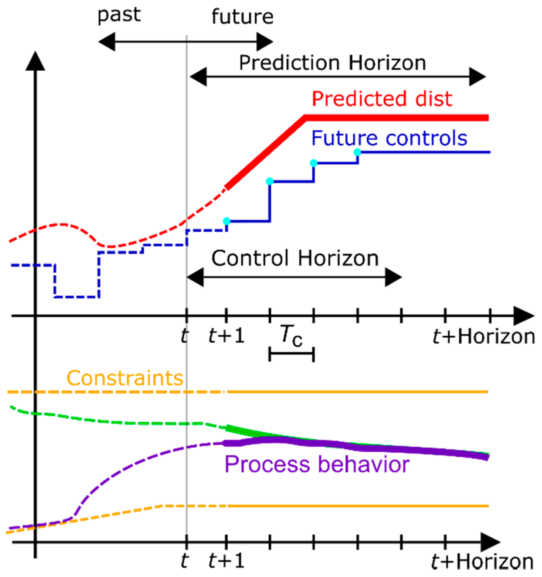
• At the control timestep $t$, MPC reads the measurements and the estimate of the current state $x_0=x\left(t\right)$ of the process. The initial state defines the simulation starting point of the controlled process;
• The optimization algorithm solves, in real time, the formulated problem for a prediction horizon of N_p time steps ahead, generating a control sequence u, which minimize the objective function J(x_t, N_p, N_c), while respecting the constraints:

  $$u=\left[\begin{array}{cccccc}u\left(1\right)& u\left(2\right)& \cdots & u\left(k\right)& \cdots & u\left(N_c\right)\end{array}\right]$$

  (21)
• The MPC acts on the controlled system, by implementing the first calculated control move u(1). The MPC keeps in memory the remaining control sequence ($k=2,\cdots N_c$) as a warm start of the optimization of the next control step.
• In the next control step, the MPC strategy comes back to step 1, by implementing a closed loop control, since the applied action on the controlled process is optimized starting from the measurement or the estimate of its current state.

The MPC formulation can be naturally extended to the more complex nonlinear case, which can be generically summarized as follows:

$$\{\begin{array}{cc}\hfill \underset{\mathit{u}}{\min }J\left(\mathit{x},\mathit{u},N_{pred}\right)=\underset{u}{\min }{\displaystyle {\displaystyle \sum }_{k=t}^{t+N_p-1}}& J\left(\mathit{x}\left(k\right),\mathit{u}\left(k\right),k\right)+E\left(\mathit{x}\left(t+N_p\right)\right)\hfill \\ \hfill \mathit{x}\left(k+1\right)& =f\left(\mathit{x}\left(k\right), \mathit{u}\left(k\right), k\right)\hfill \\ \hfill \mathit{y}\left(k\right)& =h\left(\mathit{x}\left(k\right), \mathit{u}\left(k\right), k\right)\hfill \\ \hfill \mathit{x}\left(0\right)& ={\mathit{x}}_0\hfill \\ \hfill g\left(\mathit{x}\left(k\right),\mathit{u}\left(k\right),k\right)& =0\hfill \\ \hfill l\left(\mathit{x}\left(k\right),\mathit{u}\left(k\right),k\right)& \le 0\hfill \\ \hfill r\left(\mathit{x}\left(t+N_p\right)\right)& \le 0\hfill \end{array}$$

(22)

where $J\left(\mathit{x}\left(k\right),\mathit{u}\left(k\right),k\right)$ is a generic nonlinear objective function, $\mathit{x}$ is the process state, $\mathit{u}$ is the vector of the manipulated variables, $E\left(\mathit{x}\left(t+N_p\right)\right)$ is the terminal cost,$N_p$ expresses the length of the prediction horizon, $f$ and $h$ are nonlinear functions describing the dynamic of the process state and output, $g$, $l$, $r$ are nonlinear functions describing the constraints on the system, and $r\left(\mathit{x}\left(t+N_p\right)\right)\le 0$ is named terminal constraint.

The nonlinear nature of the optimization problem leads to several issues from the computational burden point of view, which particularly differentiates the NMPC from the linear MPC case. Firstly, nonlinear optimization problems are not always characterized by convexity, and this fact does not ensure either the achievement of a global minimum, or in some cases, the convergence of optimization algorithms to a feasible solution. In the case of “simple” nonlinear problem, the main issue is calculating a solution in real-time, while ensuring a certain grade of optimality. For this reason, NMPC is less widespread and applied with respect to linear MPC. Some applications are found for slow processes, whose dynamics are compatible with calculation times. A good formulation often helps in rapidly solving the optimization problem, otherwise it is still possible to implement sub-optimal strategies [57] where the problem is feasible. A possible trade-off solution is offered by the so-called Real-Time Iteration approach [58], which implements a formulation of the optimal problem and of the optimization routines that are a “middle ground” between the linear and the nonlinear case. In cases where the real-time solution of the optimum problem is in any case not feasible, a further approach is offered by the use of methodologies called Explicit MPC, in which the optimum problem is solved offline on a discretization of the operating space of the system and is finally translated through piecewise control functions used for the online control. Interesting examples are presented by Tavernini et al. who developed an Explicit NMPC aimed at controlling antilock braking systems, implemented and tested through the Hardware-in-the-loop approach [59]; Escaño et al. applied a similar approach that combines a reduction technique based on functional principal component analysis and a fuzzy system that interpolates the output of piece-wise affine controllers [60].

3.2. PI Based Rotor Stress Controller

A preliminary implementation using a rotor stress monitor as a basis for turbine control can be obtained through a PI control strategy. The main idea behind this control approach is using an outer control ring with a first PI to create a stress set-point from turbine power current value and current set point. This set point is limited in accordance with the maximum allowed stress. The stress set-point and the stress current value are used by an inner PI in order to determine the wheel chamber pressure set-point that is compliant with the desired stress limit.

This kind of architecture is able to grant good results in terms of both production increment during start-up and stress limit compliance. An example is shown in Figure 6 where a fully cold start-up for a power gen application based on a PI rotor stress controller is compared with a standard start-up curve. In this case, the full steam header conditions allow highlighting the great advantage that can be achieved by exploiting dedicated rotor stress controller with respect to the standard startup procedures based on pre-calculated power references. In the specific case study, it is possible to increase the energy produced during the startup by over 15–20%.

At the same time, stress overshoot might appear as PI controllers are subject to fine-tuning errors. Since the effect of possible mistuning introduces the need for safety factors on the maximum allowed stress, the need of different control routines is justified (as explained in the next sections).

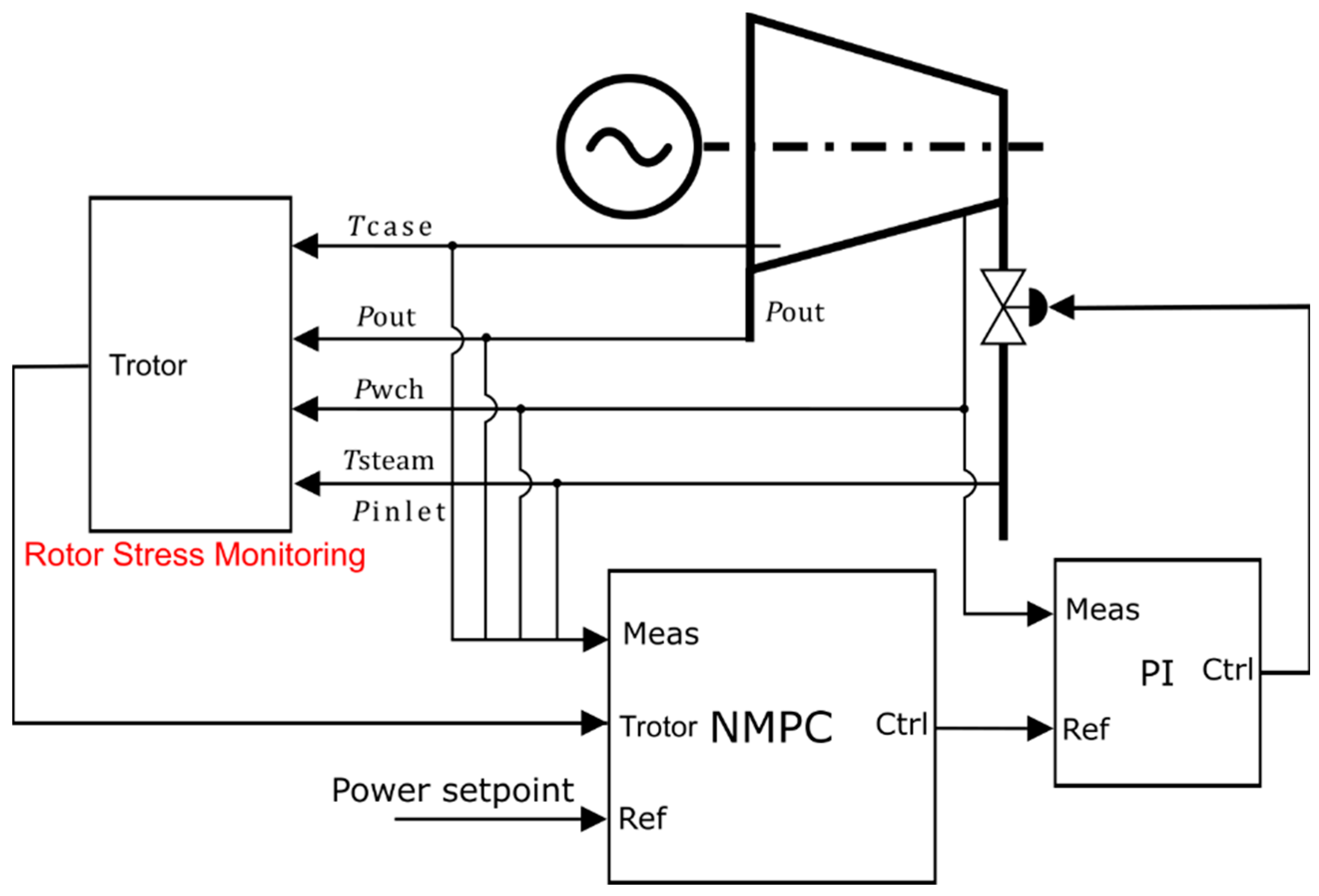
3.3. Nonlinear Model Predictive Rotor Stress Controller

The NMPC approach, shown in Figure 7, has been developed in the Matlab/Simulink environment and consists of three main software components:

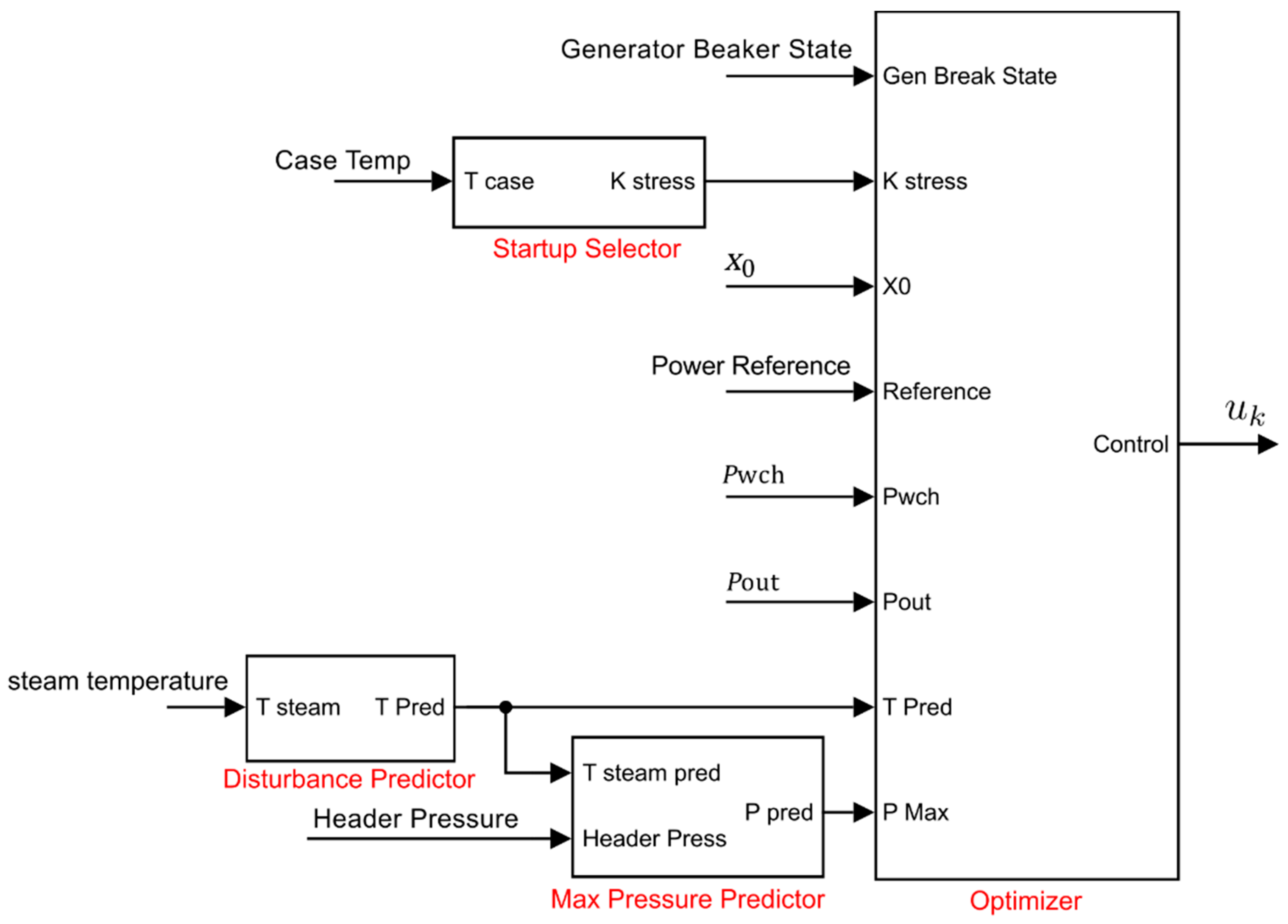
• The rotor stress monitor, i.e., the soft sensor presented in Section 2, which estimates the thermal status, focusing on the temperature of the rotor discretized in N points. The soft sensor is used as a state observer within the NMPC approach, externally installed in PLC platform as an integral part of the steam turbine governor. The block calculates the state of the machine, starting from some relevant inputs: The internal and external case temperature, the pressure and the temperature in the steam header, and the wheel-chamber and outlet pressures.
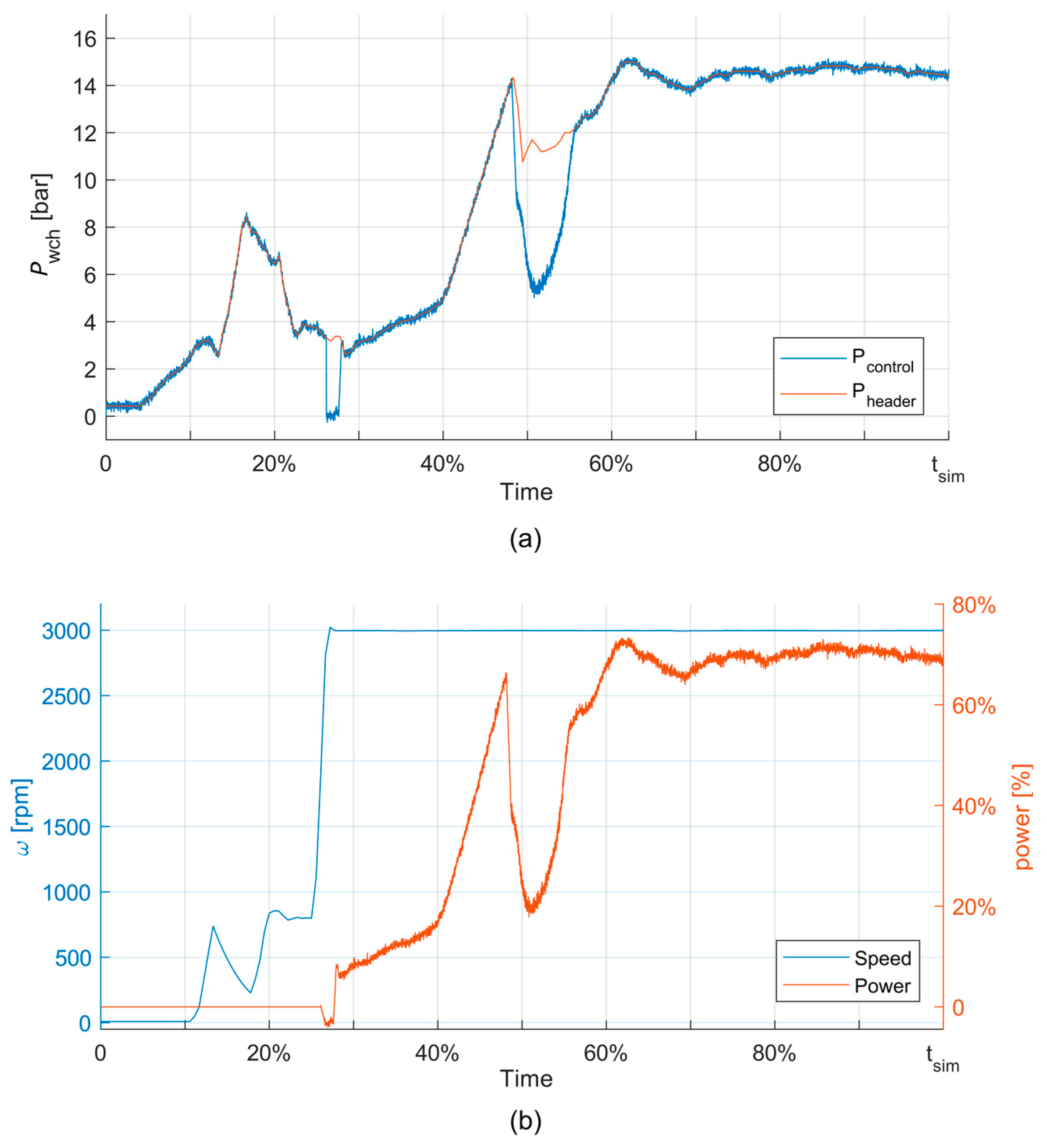
• The NMPC algorithm, which calculates a reference control action for the pressure in the wheel chamber.
• A PI controller, which directly acts on the inlet valve by following the reference from the NMPC algorithm. This particular control architecture aims at overcoming the issues related to the nonlinear behavior of the valve system, without including it in the modelling strategy formulated within the NMPC software.

The tailored NMPC application consists of 4 main blocks depicted in detail in Figure 8:

• A Startup Selector for selecting the parameters related to the maximum allowable stress according to the casing temperature and type of startup (cold, warm, hot).
• A Disturbance Predictor and a Max Pressure Predictor, which estimate, respectively, the future steam temperatures and the pressure available at the header. The steam temperature acts on the thermal dynamics as a non-controllable variable (disturbance). The predicted future header pressure is necessary to estimate its maximum constraints within the problem formulated in the NMPC. In deeper detail, the future predictions are calculated starting from the related current through a linear extrapolation. The linear extrapolation is saturated between a minimum and a maximum allowable value.
• The Optimizer, the main block of the NMPC algorithm, which implements the optimization problem, routines, and specific logics for calculating the control action. The optimization problem, formulated for a receding horizon problem, is described by the following equations:

$$\{\begin{array}{cc}\underset{\mathit{u}}{\min }{\displaystyle {\displaystyle \sum }_{k=t}^{t+N_{pred}}}\frac{1}{P_{max}^2}{\left(P_{ref}\left(t+k\right)-P\left(k\right)\right)}^T& W_P\left(P_{ref}\left(t+k\right)-P\left(k\right)\right)+\frac{1}{u_{max}^2}\mathsf{\Delta }{\mathit{u}}^T{W}_{\mathsf{\Delta }u}\mathsf{\Delta }\mathit{u}\\ \hfill \mathsf{\Delta }\mathit{u}& =\mathit{u}\left(k\right)-\mathit{u}\left(k-1\right)\hfill \\ \hfill \mathit{T}\left(k+1\right)& =\mathit{A}\left(k\right)\mathit{T}\left(k\right)+\mathit{B}\phi \left(k\right)\hfill \\ \hfill \sigma \left(k\right)& =\mathit{C}\left(k\right)\mathit{T}\left(k\right)\hfill \\ \hfill \mathit{T}\left(0\right)& ={\mathit{T}}_0\hfill \\ \hfill \phi \left(k\right)& =c\left(k\right)\cdot \mathrm{HTC}\left(k\right)\left(T_{bulk}\left(k\right)-T_N\left(k\right)\right) \hfill \\ \hfill HTC\left(k\right)& =f_1\left(u\left(k\right), T_{bulk}\left(k\right),p_{in}\left(k\right),p_{out}\left(k\right)\right)\hfill \\ \hfill P\left(k\right)& =f_2\left(u\left(k\right), T_{bulk}\left(k\right),p_{in}\left(k\right),p_{out}\left(k\right)\right)\hfill \\ & {\sigma }_{min}\left(k\right)\le \sigma \left(k\right)\le {\sigma }_{max}\left(k\right)\hfill \\ & u_{min}\left(k\right)\le u\left(k\right)\le u_{max}\left(k\right)\hfill \\ & P_{min}\le P\left(k\right)\le P_{max}\hfill \end{array}$$

(23)

where $N_{pred}$ is the prediction horizon in samples, $u$ is the manipulated variable, the pressure in the wheel chamber, $P_{ref}$ is the turbine mechanical power reference received from the DCS of the system that takes into account the current limits of the steam generation system, $W_P$ and $W_{\mathsf{\Delta }u}$ are, respectively, the weight for the reference tracking and the variation of the control action, $f_1$ and $f_2$ are nonlinear functions, which describe the relationships between the main thermodynamic variables of the ST and HTC and the generated mechanical power $P$, respectively, and ${\sigma }_{min}$ and ${\sigma }_{max}$ are respectively the minimum and maximum limits of the stress, designed in function of the specific mission of the turbine.

The control sequence $\mathit{u}=\left[\begin{array}{cccc}{u}_1& u_2& \cdots & u_{N_X}\end{array}\right]$ is calculated with a blocking strategy, in which the $N_X$ calculated variables are spatially distributed along the prediction horizon (such as shown in Figure 9) and linearly interpolated in the intermediate points with a sampling time $T_{\mathrm{s}}$, which also discretizes the dynamics of the thermic rotor model. With respect to standard blocking strategies, which concentrate the control action in the beginning of the control horizon, the presented approach aims at limiting the peak of stress for the whole prediction horizon, in order to overcome issues related to the infeasibility of the optimization problem due to a short control horizon.

The presented formulation is characterized by a large number of constraints mainly due to the evaluation of machine dynamics every $T_{\mathrm{s}}$ for the aforementioned stability issues. In order to reduce the computational burden, two strategies have been implemented within the NMPC algorithm. The first one concerns the decimation of the number of power and stress constraints evaluation along the prediction horizon. The second one concerns the scheduling of the optimizer with a frequency lower than the frequency relative to the model simulation sampling time.

In detail, the decimation of evaluation of stress constraints is motivated by the fact that the stress dynamics follow the thermal ones and are therefore slow. For this reason, it is possible to evaluate the constraints every $k_{cd}{T}_s$ seconds, where $k_{cd}$ is the decimation parameter:

$${\sigma }_{min}\le \left[\begin{array}{cccccc}\sigma \left(k\right)& \sigma \left(k+k_{cd}\right)& \cdots & \sigma \left(k+n{k}_{cd}\right)& \cdots & \sigma \left(N_{pred}\right)\end{array}\right]\le {\sigma }_{max}$$

(24)

The power constraints are evaluated in the same way, as their dynamics are bound by the limitation on the wheel chamber pressure, which is in turn limited by stress-derived limits. A well-tuned decimation parameter $k_{cd}$, allows a considerable reduction of the number of constraints on stress and computational costs.

The second strategy implements the decimation of the frequency of the optimizer respect to the NMPC frequency $f_c$:

$$f_c=\frac{1}{T_c};T_c=T_{\mathrm{s}}$$

(25)

The optimizer is scheduled with a frequency $f_{opt}$ multiple of the NMPC scheduling frequency:

$$f_{opt}=\frac{1}{T_{opt}};T_{opt}=k_{\mathrm{mpc-period}}{T}_c$$

(26)

A well-tuned $k_{\mathrm{mpc-period}}$ parameter allows overcoming the limitation concerning the fact that the optimizer computational cost is not compatible with the controller frequency.

The optimizer routine is based on the SQP algorithm [61]. In particular, in this work, two different implementations have been used: The Matlab fmincon routine used as a benchmark, and a tailored Sequential Quadratic Programming (SQP) approach, which is license-free as it was ad-hoc developed.

3.4. Tailored SQP Algorithm

SQP is a state-of-the-art algorithm that allows solving general nonlinear optimization problems in the form:

$$\{\begin{array}{c}\min f\left(x\right)\\ c\left(x\right)=0\\ b\left(x\right)\le 0\end{array}$$

(27)

where $f\left(x\right), b\left(x\right), c\left(x\right)$ are generic non-linear functions. Nonlinear optimization is an NP-hard problem, namely it is computationally expensive to solve. The basic idea of SQP is to form quadratic sub-problems that are computationally easier and iteratively solve them in order to converge to a solution of the global problem. The approach followed is similar to the one proposed in [62].

Let:

$$\mathrm{L}\left(\mathrm{x},\sigma ,\lambda \right):=f\left(x\right)+{\sigma }^{\prime }\cdot c\left(x\right)+{\lambda }^{\prime }\cdot b\left(x\right)$$

(28)

be the Lagrangian of the problem. Let $H\left(x\right)$ be the Hessian of $\mathrm{L}\left(x,\sigma ,\lambda \right)$ as a function only of $x$ at some fixed values of $\left(\sigma ,\lambda \right)$. Let $\mathsf{\Delta }f$ be the gradient of the function $f$ and ${\mathrm{J}}_b,{ \mathrm{J}}_c$ the Jacobians of the functions $b,c$. The sub-problem to solve at iteration k is formulated as follows:

$$\begin{array}{c}\min \frac{1}{2}{d}^{\prime }\cdot H\left(x_k\right)\cdot d+\mathsf{\Delta }f\left(x_k\right)\cdot d\\ {\mathrm{J}}_c\left(x_k\right)\cdot d+c\left(x_k\right)=0\\ {\mathrm{J}}_b\left(x_k\right)\cdot d+b\left(x_k\right)\le 0\end{array}$$

(29)

The expression is a quadratic problem in the variable $d$, positive definite since $H\left(x_k\right)$ is kept positive definite. The solution $d_k$ to the quadratic sub-problem provides the direction of improvement at the next iteration of the original problem solution:

$$x_{k+1}=x_k+d_k$$

(30)

To improve the convergence, the step length $\alpha$ is calculated in order to update the solution:

$$x_{k+1}=x_k+\alpha \cdot d_k$$

(31)

where $\alpha$ is computed by optimizing a merit function.

If stopping conditions or constraints violation are satisfied, the current solution is given as output. Otherwise, a new iteration is performed. This algorithm converges to a minimum of the objective functions [62] and performs fast iterations, since the quadratic sub-problem is convex at every iteration: Convex quadratic problems can be solved in polynomial time. For this purpose, an active set method has been exploited; the problem is iteratively solved starting from a feasible initial solution calculated with the simplex method. At every iteration, a sub-problem taken only on some equality (active) constraint is solved through QR matrix decompositions [63]. The solution is then iteratively updated in a way that preserves feasibility. This procedure converges in polynomial time to the optimum of the quadratic sub-problem.

With respect to the fmincon routine, the tailored algorithm manages the tolerance on constraints, solutions, and jacobian in a different way. The algorithm tries to converge starting from a minimum allowed tolerance and increasing it of a factor if it is not respected at the end of the number of allowed iterations.

In order to make this algorithm implementable on a PLC platform in the future, the algorithm has been developed in the Matlab environment and the opportunity of translating it into the PLC native language through the PLC Coder Toolbox has been tested. As many Matlab routines (such as the fmincon function, the linear(quadratic) solvers, etc.) cannot be directly translated by the PLC Coder, in their place, the above tailored algorithms have been coded and used. The SQP implementation has been tested with respect to Matlab fmincon for several problems and showed similar or sometimes even better performances. In particular, the two algorithms behave similarly on instances of the nonlinear problem arising from the NMPC. With respect to the fmincon routine, the tailored SQP algorithm for PLC platforms is currently 8–10 times slower.

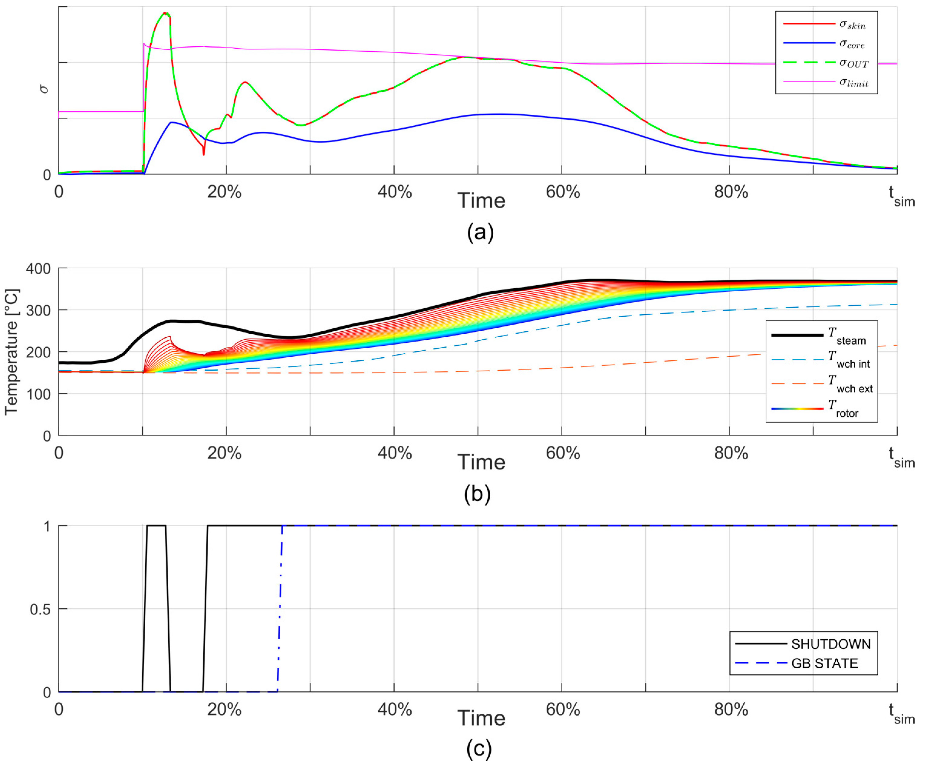
4. Results

Extensive simulation studies have been performed, through which the performance of the proposed NMPC approach has been compared to the selected benchmark based on the PI Controller as well as to a second benchmark based on the standard procedures for power startup, based on pre-calculated load curves. In order to assess the validity of the NMPC approach, all the control approaches have been simulated by using real data related to a Low-Pressure (LP) ST with a rated power of 45 MW, an inlet steam pressure of 1–22 Bar, an inlet steam temperature of 180–380 °C, and a rated speed 3000 RPM. The external radius is assumed to be equal to 29.5 cm in the equivalent cylindrical model and the rotor is assumed to be made of ferritic-martensitic heat resisting forged steel for power generation applications. Even if material properties cannot be disclosed, similar results can be obtained assuming material properties of A470 class 8 whose data are easily available, for example in the NIMS database. It has to be remarked that these material properties are not fundamental to quantify the goodness of the control strategy (a start-up performed with a worse-performing rotor material determines a longer start-up but does not invalidate the control strategy performance). The machine is discontinuously operated in a CSPP, where the steam characteristics vary as a function of the weather with numerous starts per year. The specific case study is related to a cold startup of a typical winter day, during which the steam does not reach the full header conditions in terms of mass flow and enthalpy with respect to the maximum potential of the plant. The steam characteristics are depicted in Figure 10: The top diagram shows the pressure on the steam header (in blue), the temperature of the inlet steam (red line), and the internal and external temperatures of the LP machine casing (green and orange lines, respectively); the central diagram depicts the rotor speed, while the bottom diagram shows the startup command (blue line) and the state of the generator breaker (orange line). For confidentiality constraints, the time axes are dimensionless.

The control performance has been evaluated through three main indexes, related to the maximum percentage stress overshoot, the generated mechanical energy during the startup, and the computing time. Firstly, the performance of PI controller has been evaluated with respect to the standard startup procedures, starting from a brief discussion related to the controller parameter selection. In a second phase of the work, extensive tests have been performed on the NMPC approach, in order to evaluate the performance sensitivity related to the main controller parameter.

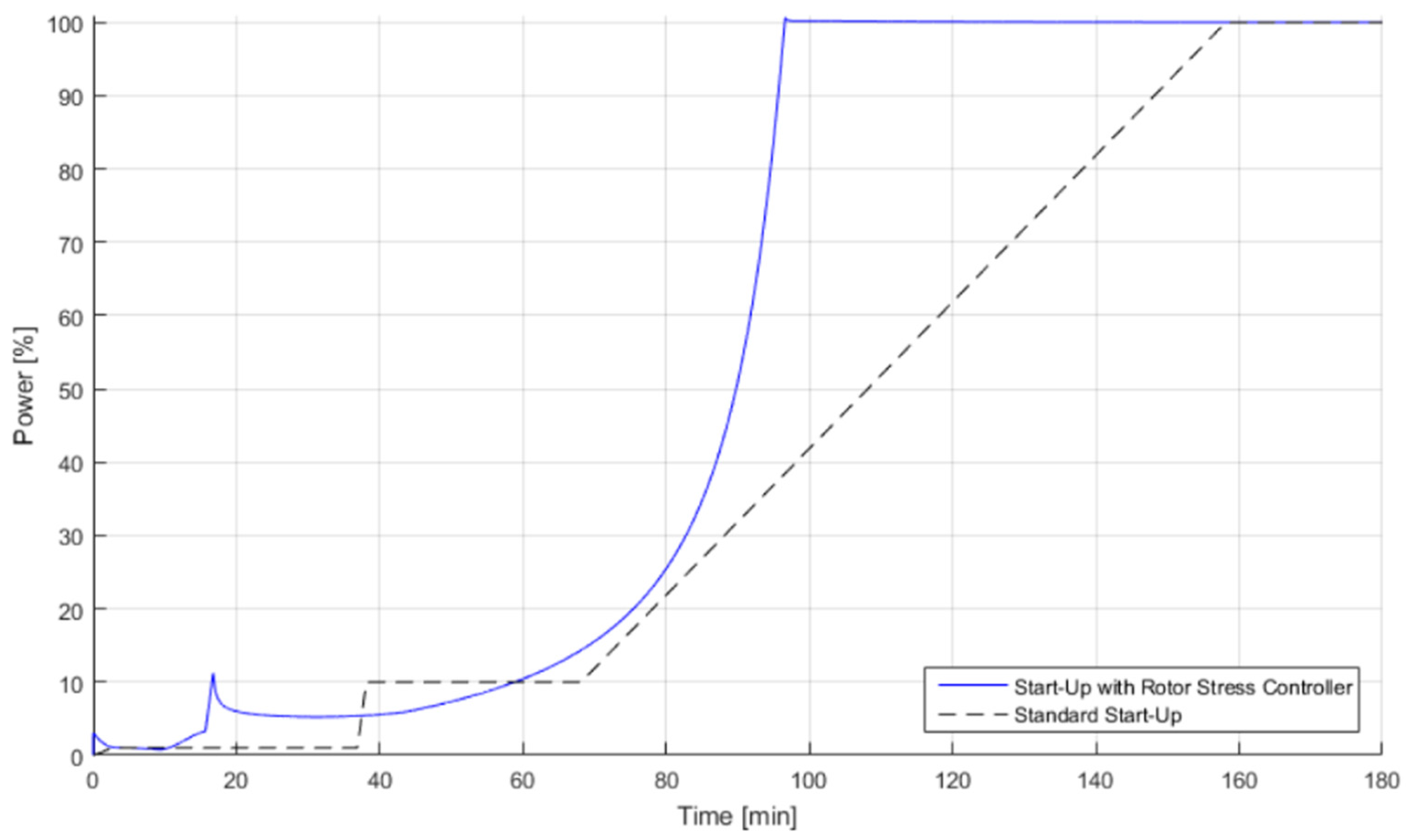
4.1. PI Control Results

In order to assess the performances of the PI based controller, it is important to verify the sensitivity of this kind of controller to a possible mistuning of its gain parameters. It has to be remarked that during commissioning the gain parameters of power PI are usually modified to obtain the desired control performances. In this scenario, the control architecture should have pre-set values enabling a faster commissioning. A sensitivity analysis based on a Design of Experiments approach solves this kind of problem with the main objective of identifying the optimal gain values of the internal stress PI. In more detail, the controller has been initially tuned through a proprietary site procedure similar to ZN methodologies, adapted to the constraints of the site itself. In addition, a sensitivity analysis was carried out on the performance, in terms of generated energy and stress overshoot, as the controller parameters varied, in a large neighborhood of the operative point identified by the site procedures, in order to verify the robustness of the methodologies applied to the specific case. The results of the sensitivity analysis are shown in Figure 11 where the energy production and the maximum percentage overshoot are shown.

The results of the DoE show that the peak production also corresponds to the maximum stress overshoot. The results show that the overshoot peak cannot be fully eliminated unless heavily scarifying the performances through a very large integral coefficient of the PI Controller. The solution requires introducing an additional safety factor on the maximum allowable stress for the turbine rotor, in order to limit the stress reference on the PI controller, with a consequent limited reduction of the energy production during start-up. An example of this behavior is shown in Figure 12 and Figure 13 where the PI intervention can be clearly identified between 48–65% of the simulation time $t_{sim}$.

In particular, in Figure 12, the top diagram shows the equivalent rotor stress in the core (red), the rotor skin stress (blue), the maximum between core and skin stress (green), and the maximum allowable rotor stress in violet. The bottom figure shows the steam temperature in black, the temperature of the external and internal casing (dashed lines in orange and yellow), and the temperature of the rotor in different point of the radius (from blue in the core to red in the skin). In Figure 13, the top diagram shows the controlled steam pressure in the wheel chamber (blue) and the available pressure in the header (orange). The bottom figure shows the rotor speed in blue and the mechanical power in the turbine shaft normalized with respect to the rated power.

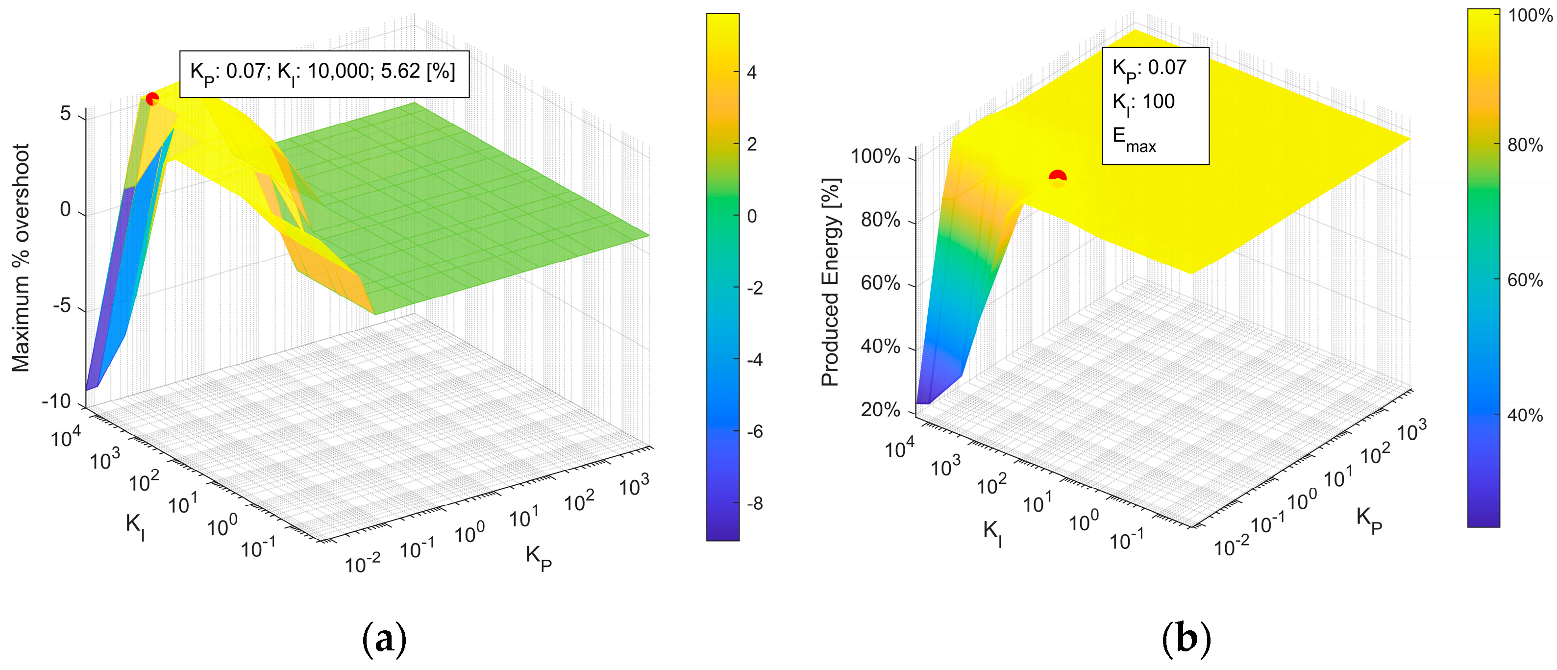
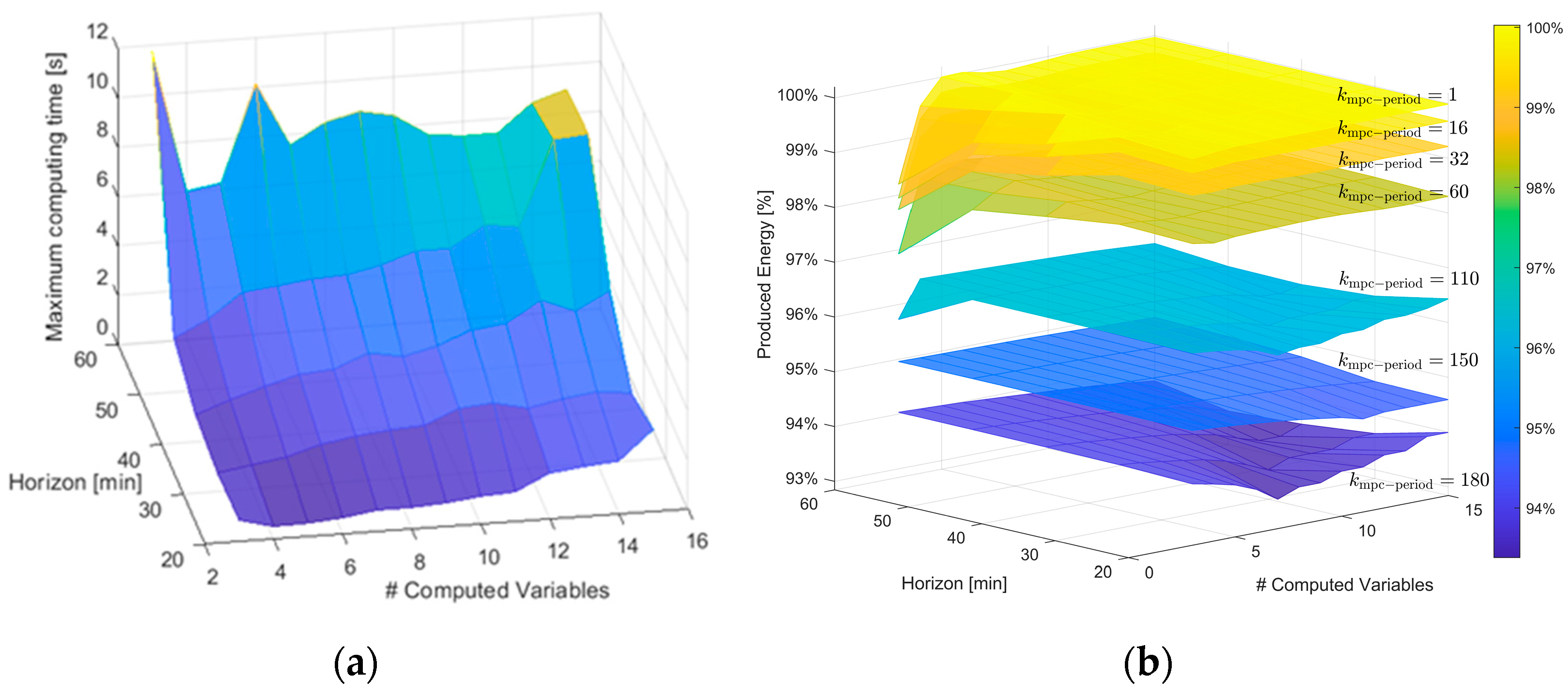
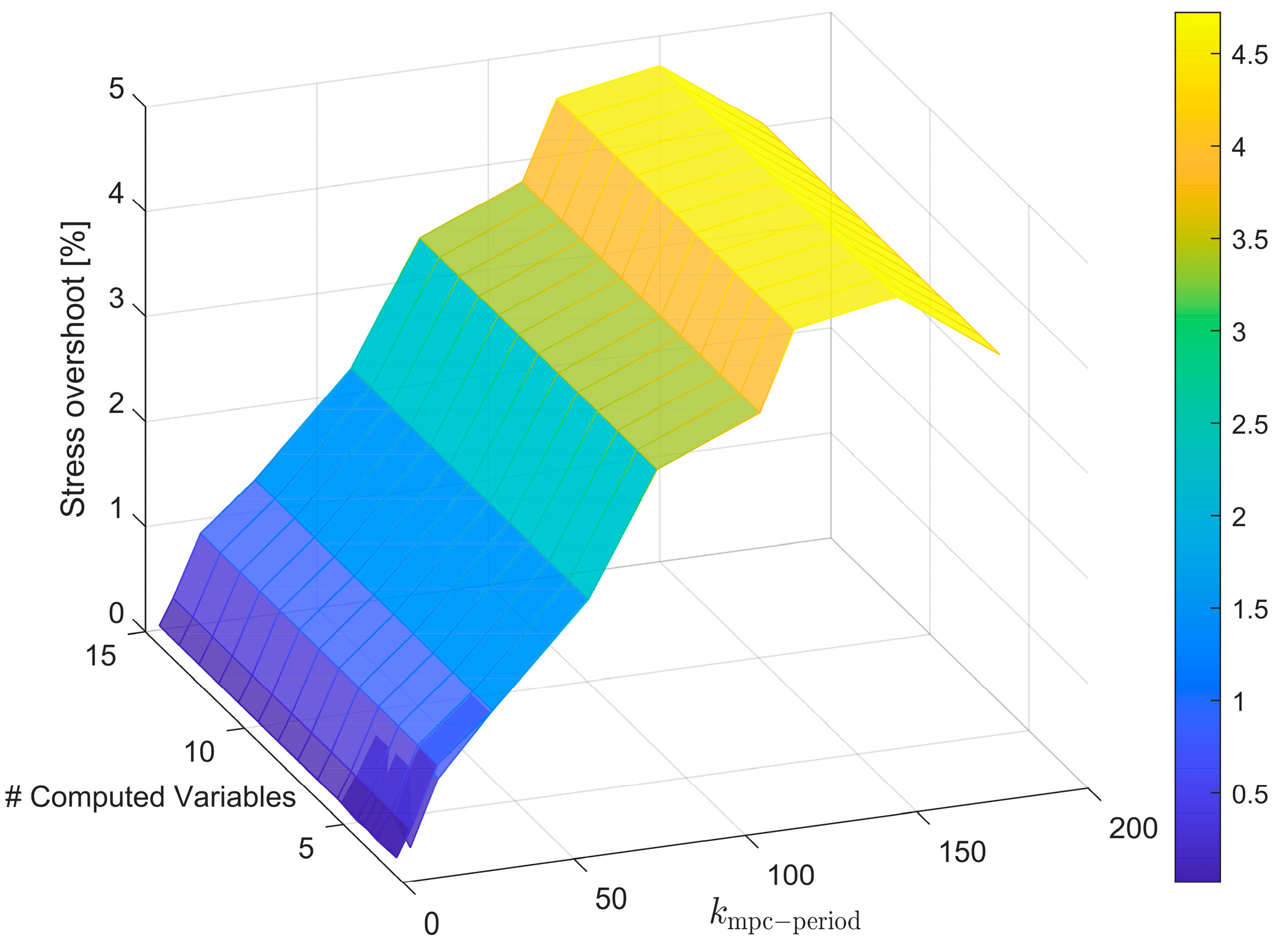
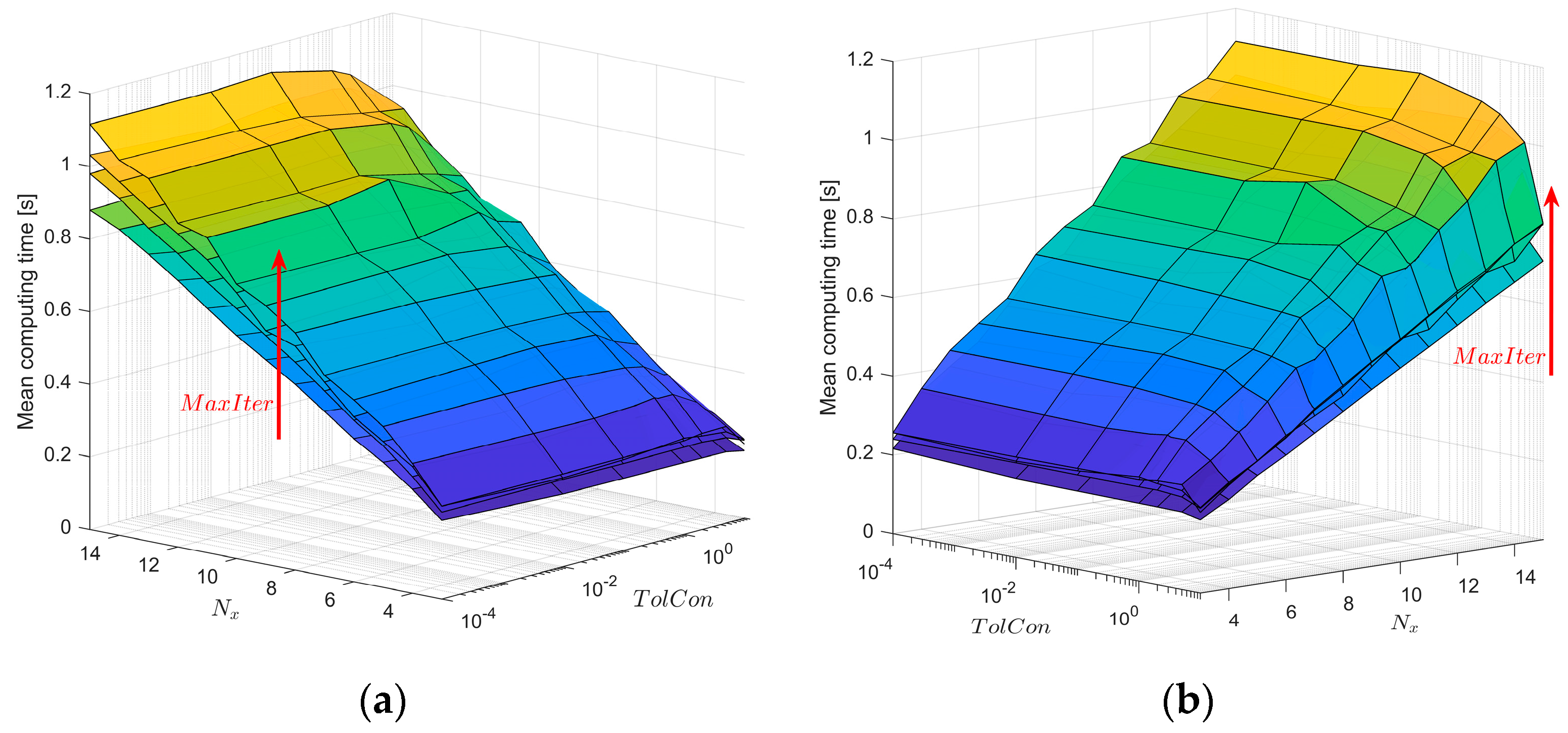
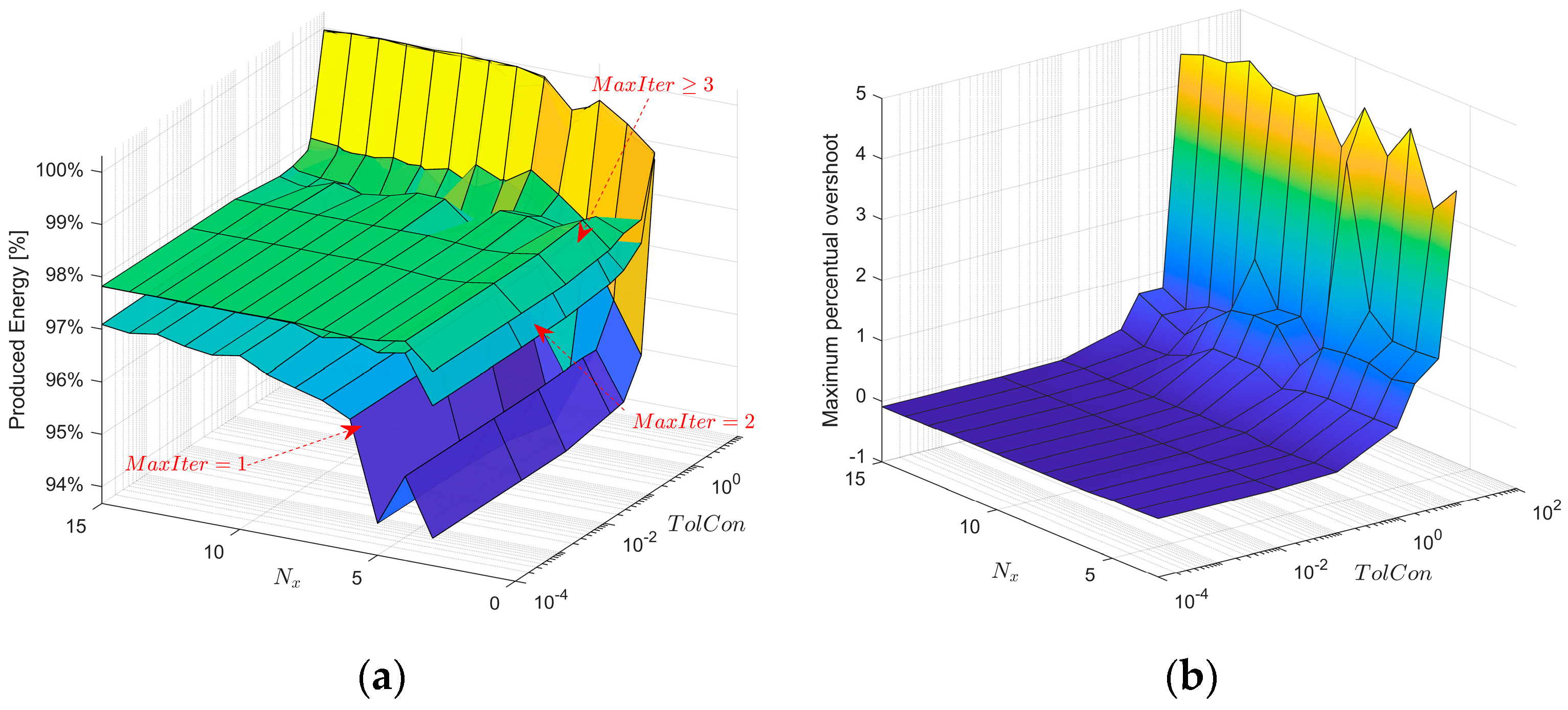
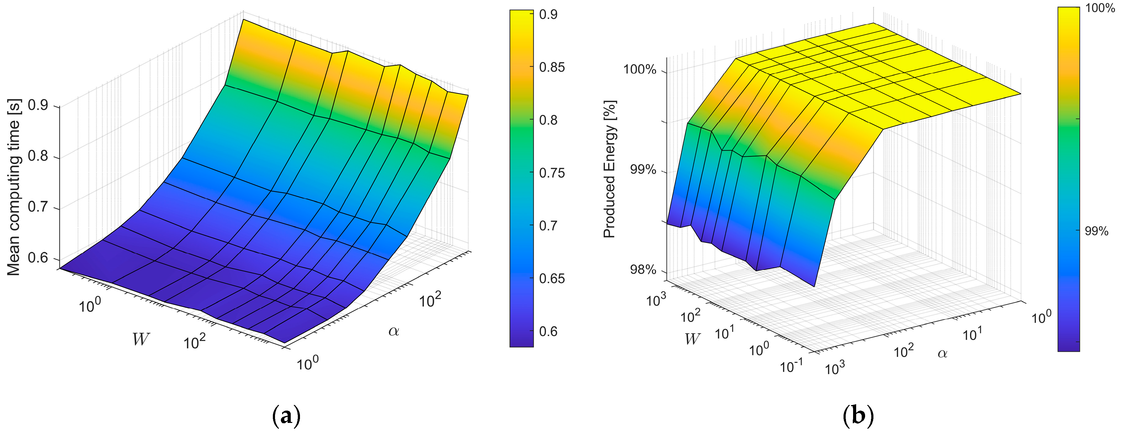
4.2. DOEs NMPC

This section presents the outcomes of the main tests on the NMPC, which were aimed at evaluating the performances of this approach related to both energy production and startup speed up and viability in terms of computing time. In particular, the extensive test campaign mainly focuses on balancing the control performances and the heavy computation burden of NMPC, with the objective of finding an optimal configuration of its parameters. Among the different tests that have been performed, we present here the main results related to the sensitivity analysis with respect to control, optimizer, and formulation parameters (namely, cost function parameters). In particular, the following parameters are considered:

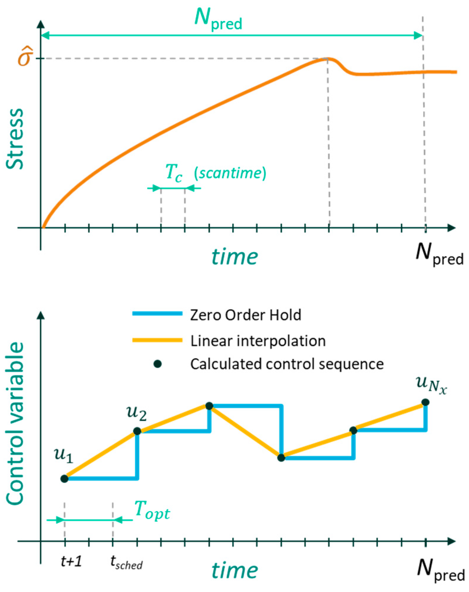
• Time-related parameters $N_x, N_{pred},k_{\mathrm{mpc-period}}$, in which, when $k_{\mathrm{mpc-period}}>1$ (the optimizer is not scheduled every control step), the control action is kept constant through a sample and hold strategy;
• Main optimizer parameters $N_x$, MaxIter and TolCon;
• Cost function weights, $W_p$ and $W_{\mathsf{\Delta }u}$, where $W$ and $W_{\mathsf{\Delta }u}$ have been varied according to the relationships: $W_{\mathsf{\Delta }u}=\alpha W$, $W_p=W;$

The abovementioned tests are summarized through three different figures. In the figures, the energy is normalized with respect to the maximum energy produced resulted in the specific DoE related to the NMPC application to the case study. Figure 14 and Figure 15 are related to the first test campaign. In particular, Figure 14a shows the maximum calculation time as a function of the prediction horizon and the number of calculated variables $N_x$, which highlights an evident link between the hyperparameters involved and the calculation time. The calculation time appears to be very sensitive to the prediction horizon and slightly less sensitive to the number of variables calculated. Figure 14b shows the produced energy as a function of the varied parameters, in particular highlighting a great sensitiveness to the frequency of the optimizer and an increasing sensitivity with respect to the prediction horizon and the number of calculated freedom degrees when the optimizer is more frequently scheduled ($k_{\mathrm{mpc-period}}\in \left[1, 32\right])$. Figure 15 shows the percentage stress overshoot as a function of the varied parameters. In particular, the graph shows that the overshoot depends only on the optimizer scheduling frequency, due to the fact that a sample and hold strategy for a less frequent optimizer activity is not efficient.

Figure 16 and Figure 17 show the results related to the second test campaign, where $N_x$, MaxIter and TolCon are varied. In particular, Figure 16a,b shows the mean calculation time as a function of the main optimizer parameters, highlighting that it is substantially dependent on $N_x$ and less dependent on the number of iterations. As the tolerance on the constraints increases, the calculation time decreases in terms of both average and maximum time, as the optimizer relaxes the constraints more. Figure 17a shows the produced energy in function of the varied parameters, which is dependent on the tolerance on the constraints TolCon. With a number of maximum iterations MaxIter equal to 1, the surface shows a dependence also on $N_x$. Figure 16b shows the percentual stress overshoot in function of the varied parameters, and in particular, that overshoot mainly depends on the tolerance constraints and slightly on $N_x$.

Figure 18 shows the results related to the third test campaign, which investigates the effect of the cost function weighs on the control performance. Figure 18a depicts the mean computing time in function of the varied parameters, while Figure 18b shows the produced energy. The test shows that both computing time and produced energy highly depend on $\alpha$ (and, therefore, on $W_{\mathsf{\Delta }u}$).

4.3. Guidelines for Controller Parameters Tuning and Discussion of Results

The analysis clarifies the main dependence relationships between the NMPC parameters and the resulting performance. As mentioned before, three main aspects have to be considered: (i) The performance in terms of produced energy; (ii) the overshoot of stress; and (iii) the computation burden.

In first place, the energy produced depends on a decreasing proportion of the frequency of scheduling of the optimizer, the maximum number of iterations MaxIter, the number of control freedom degrees $N_x$, and the length of the prediction horizon $N_{pred}$. In more detail, the energy is substantially dependent on the frequency of scheduling of the optimizer: The less frequently the optimizer is scheduled, the less the controller is capable of optimizing the starting curve of the machine. The produced energy is also partially dependent on the combination of the maximum number of iterations and the number of Degrees of Freedom (DOFs) of the control. For a low number of maximum iterations (i.e., MaxIter = 1), the produced energy highly depends on the number of control DOFs. The greater $N_x$, the greater the amount of produced energy, since fewer iterations are, however, balanced by a greater number of variables, which allow better optimization of the control action. For a maximum number of iterations greater than 3, it is possible to obtain the maximum possible energy during start-up (if the tuning of the other parameters is optimal). Finally, the prediction horizon $N_{pred}$ slightly affects the produced energy, due to the accuracy of disturbance predictions, which is less accurate for a long prediction horizon. The computational cost mainly depends on the length of the time horizon $N_{pred}$, on the number of future variables that are controlled $N_x$, and, finally, on the parameter $W_{\mathsf{\Delta }u}$, which weights the variation of control action between consecutive control steps. The tolerance on constraints TolCon has a role on the sensitivity analysis but only when this is rather high, resulting in a decreased computational cost. In deeper details, high values of $N_{pred}$, $N_x$, and $W_{\mathsf{\Delta }u}$ lead to higher computational costs. In conclusion, these four parameters must be carefully tuned for first. The length of the prediction horizon must cover the rise time of the stress in order to predict and identify the peak of stress, and, at the same time, it is necessary to balance the counteracting calculation time. Ultimately, this important parameter depends on the construction material of the machine and its size. Once the abovementioned parameters are tuned, the required computation burden—in terms of maximum computation time—can be balanced by tuning the frequency of the scheduling of the optimizer. The maximum percentage stress overshoot mainly depends on the scheduling frequency of the optimizer and on the tolerance of the optimization algorithm on constraints. The overshoot is almost linearly dependent on the two parameters.

An example of fine-tuned NMPC controller application is shown in Figure 19, Figure 20 and Figure 21. More in detail, the simulation is performed with a sampling time $T_{\mathrm{s}}=2$ s, a prediction horizon of 40 min ($N_{pred}=$ 1200 samples) and a number of control steps equal to $N_x=$ 5. The optimizer within the NMPC has been scheduled every $k_{\mathrm{mpc-period}}=$ 4 periods, equal to 8 s, to guarantee an adequate margin for the computation time. Figure 19 shows on the top diagram the stress during start-up (blue in the core, red in the skin of the rotor, green the maximum stress) and the stress limit (in purple). The middle diagram depicts the temperature of the steam in the header (black), the temperature of the external and internal casing (dashed lines in orange and yellow), and the rotor temperature in each radial node (from blue in the core to red in the skin). The bottom diagram shows the state of the generator breaker (blue) and the start-up state (black). Figure 20 shows, in the top diagram, the pressure on the header (yellow) and the regulated pressure in the wheel chamber (blue). The middle diagram shows the rotor speed (blue) and the generated mechanical power (orange). Figure 21 depicts the computing time of the scheduled optimizer in the NMPC.

The simulation shows several interesting results. The control mission shows two singular behaviors: The first one occurs around 11–17% of simulation time, when a peak in the rotor stress is observed, which is due to the speed startup and is not controllable by the NMPC that acts on the power startup. The second one occurs around 47–53% of simulation time, when the NMPC effectively regulates the wheel chamber pressure in order to limit the thermal stress conditions in the rotor without overshoots on the rotor stress behavior.

The comparison between the NMPC and PI control strategies shows several interesting results.

Table 1. Control results. Comparison between proposed approaches (PI RSC and NMPC).

Case Study	NPIAE	NPC
PI RSC with overshoot	4.77	95.23
PI RSC no overshoot	5.30	94.70
Tuned NMPC	2.49	97.51

summarizes the main numerical results for the three case studies: (i) PI Rotor Stress Controller; (ii) PI Rotor Stress Controller with anti-overshoot; and (iii) well-tuned NMPC. All the case studies refer to the control of the steam in CSPP application, in which the steam header condition is dependent on the weather condition, and rarely reach the full header capacity in terms of temperature and pressures. The results are reported in terms of two different indexes: The Normalized Percentual Integral Absolute Error (NPIAE) and the Normalized Production Capability (NPC) that describes the ratio between the produced energy in the case of controlled rotor stress scenario and the maximum theorical energy production. The NPIAE is a normalized version of the IAE index to overcome confidentiality data issues related to the intellectual property.

$$\mathrm{NPIAE}=100\frac{{{\displaystyle \int }}_{t_o}^{t_{end}}\left|P_{\max }\left(t\right)-P_{s_i}\left(t\right)\right|}{{{\displaystyle \int }}_{t_o}^{t_{end}}\left|P_{\max }\left(t\right)\right|}$$

(32)

$$\mathrm{NPC}=100\frac{E_{s_i}}{E_{\max }}$$

(33)

where $P_{s_i}\left(t\right)$ is the power produced at the time $t$ for the presented $i$-th control scenario, $P_{\max }$ is the power produced in a scenario with uncontrolled rotor stress, $t_o$ and $t_{end}$, respectively, are the initial power startup time and the instant in which the startup ends, and $E_{s_i}$ and $E_{\max }$ are, respectively, the energy produced in the $i$-th controlled scenario and the uncontrolled scenario.

In particular, the NMPC allow one to totally avoid the stress overshoot, which in some control applications, can result in poor or dangerous behaviors, while through the PI controller it is not possible to eliminate the overshoot unless one adequately limits the stress reference with safety factors (as in the second scenario). Safety factors in fact limit the energy production during the startup. Another fundamental aspect concerns the production of energy during the startup. The PI controller application shows encouraging results, considering the simplicity of the control implementation. In conditions of perfectly tuned NMPC and PI controllers, in the presented case study, the NMPC allows one to produce about 2.3% more energy than the PI-based rotor stress controller. In turn, the controller allows one to increase energy production by over 15–20% compared to what can normally be obtained with pre-calculated load curves.

In general, PI tuning is a difficult task in practice, which is performed by field engineers who usually exploit conservative tuning methodologies. NMPC tuning can be performed offline through an automatic simulation campaign, with relevant savings of commissioning time. In this context, NMPC overcomes not only several issues related to overshoot managing, but also the PI controller mistuning issues, resulting in superior performance.

5. Conclusions

In this paper, an extensive presentation of a Nonlinear Model Predictive Control approach has been presented and compared with respect to the standard control methodologies for speeding up the power startup of steam turbines. The NMPC approach includes a detailed thermodynamical model of the machine that allows to identify with a great accuracy the thermal behavior of its rotor, in particular focusing on the equivalent stress.

A final analysis of the obtained results and the comparison of the proposed advanced control approach to standard ones show that relevant improvements can be achieved by using NMPC architecture. Firstly, the NMPC—when well-tuned with offline procedures—guarantees a total rejection of the stress overshoots and superior performances in terms of produced energy, with respect to both start-up through pre-calculated curves and the PI controller. In order to prove the effectiveness of the proposed approach, the application to a specific case study was presented regarding the startup of steam turbines in concentrated solar power plants, characterized by particularly variable steam conditions. For this specific application, when the PI controller action is tuned to eliminate stress overshoots, the NMPC gains about 2.3% in terms of energy produced during the startup, on top of the 15–20% output power gain that can be obtained through a standard PI control scheme aimed at thermal stress containment with respect to standard start-up curves.

The only bottleneck in applying NMPC methodologies when starting small machines is the calculation time, which currently does not guarantee application on PLC platforms, except through complex distributions of the optimization calculation on consecutive control cycles. Real-Time Iteration architecture may overcome these issues and will be the object of future developments of this topic.

Future work will aim at developing an adaptive blocking strategy, based on the current thermal state and the stress of the machine. In particular, the strategy can be effectively adjusted through Fuzzy Logic-based methodologies that can vary both the number of DOFs and their concentration over time in order to favor a better optimization of the starting curve in its initial moments and a further reduction of the calculation times. A further increase in performance can be obtained by improving the disturbance models that forecasts the steam characteristics at the inlet of the turbine, along the prediction and control horizons of the NMPC. An accurate model of the available steam energy at the inlet is necessary to improve the MPC performances, as it allows one to obtain less restrictive and conservative control curves. Furthermore, a broader point of view on the startup issues faced in a global way could allow to further increase the performance. On the one hand, the control system can be extended to the generation of steam itself, with enormous benefit on the synchronization of the machines and the plant, at the cost of a higher computational burden. On the other hand, the modeling work can be extended in the same point of view, with a greater number of details and consequent precision of the predictions of the vapor characteristics. AI techniques, e.g., Recurrent Neural Networks-based architectures, can undoubtedly improve the prediction of future disturbances and make the start-up curve less conservative. Interesting examples are systems based on concentrated solar thermal technology, in which AI methodologies can certainly benefit from the use of AI techniques for prediction of steam characteristics based on weather data and the condition of the solar field plant, in order to improve not only the management of connected STs but also the overall performance.

References

- Kondziella, H.; Bruckner, T. Flexibility requirements of renewable energy based electricity systems—A review of research results and methodologies. Renew. Sustain. Energy Rev. 2016, 53, 10–22. [Google Scholar] [CrossRef]
- Siano, P. Demand response and smart grids—A survey. Renew. Sustain. Energy Rev. 2014, 30, 461–478. [Google Scholar] [CrossRef]
- Mathiesen, B.V.; Lund, H.; Connolly, D.; Wenzel, H.; Østergaard, P.A.; Möller, B.; Nielsen, S.; Ridjan, I.; Karnøe, P.; Sperling, K.; et al. Smart energy systems for coherent 100% renewable energy and transport solutions. Appl. Energy 2015, 145, 139–154. [Google Scholar] [CrossRef]
- Tascioni, R.; Arteconi, A.; Del Zotto, L.; Cioccolanti, L. Fuzzy logic energy management strategy of a multiple latent heat thermal storage in a small-scale concentrated solar power plant. Energies 2020, 13, 2733. [Google Scholar] [CrossRef]
- Badami, V.; Chiang, K.; Houpt, P.; Bonisonne, P. Fuzzy logic supervisory control for steam turbine prewarming automation. In Proceedings of the 1994 IEEE 3rd International Fuzzy Systems Conference, Orlando, FL, USA, 26–29 June 1994; Institute of Electrical and Electronics Engineers (IEEE): New York, NY, USA, 2002. [Google Scholar]
- Carnero, A.P.; Serrano, L.R.; Nebradt, J.G.; Leyva, L.M. Integration of thermal stress and lifetime supervision system of steam turbine rotors. Combust. Fuels Emiss. Parts A B 2008, 3, 1035–1044. [Google Scholar] [CrossRef]
- Sun, Y.-J.; Liu, X.-Q.; Hu, L.-S.; Tang, X.-Y. Online life estimation for steam turbine rotor. J. Loss Prev. Process. Ind. 2013, 26, 272–279. [Google Scholar] [CrossRef]
- Rusin, A.; Nowak, G.; Lipka, M. Practical algorithms for online thermal stress calculations and heating process control. J. Therm. Stress. 2014, 37, 1286–1301. [Google Scholar] [CrossRef]
- Banaszkiewicz, M. Online monitoring and control of thermal stresses in steam turbine rotors. Appl. Therm. Eng. 2016, 94, 763–776. [Google Scholar] [CrossRef]
- Banaszkiewicz, M.; Dominiczak, K. A methodology for online rotor stress monitoring using equivalent Green’s function and steam temperature model. Trans. Inst. Fluid-Flow Mach. 2016, 133, 13–37. [Google Scholar]
- Dominiczak, K.; Rządkowski, R.; Radulski, W.; Szczepanik, R. Online prediction of temperature and stress in steam turbine components using neural networks. J. Eng. Gas Turbines Power 2016, 138, 052606. [Google Scholar] [CrossRef]
- Casella, F.; Pretolani, F. Fast start-up of a combined-cycle power plant: A simulation study with Modelica. In Modelica Conference; The Modelica Association: Linköping, Sweeden, 2006; Volume 4. [Google Scholar]
- Faille, D.; Davelaar, F. Model based start-up optimization of a combined cycle power plant. IFAC Proc. Vol. 2009, 42, 197–202. [Google Scholar] [CrossRef]
- Sun, Y.-J.; Wang, Y.-L.; Li, M.; Wei, J. Performance assessment for life extending control of steam turbine based on polynomial method. Appl. Therm. Eng. 2016, 108, 1383–1389. [Google Scholar] [CrossRef]
- Boulos, A.M.; Burnham, K.J. A fuzzy logic approach to accommodate thermal stress and improve the start-up phase in combined cycle power plants. Proc. Inst. Mech. Eng. Part B J. Eng. Manuf. 2002, 216, 945–956. [Google Scholar] [CrossRef]
- Matsumoto, H.; Ohsawa, Y.; Takahasi, S.; Akiyama, T.; Hanaoka, H.; Ishiguro, O. Startup optimization of a combined cycle power plant based on cooperative fuzzy reasoning and a neural network. IEEE Trans. Energy Convers. 1997, 12, 51–59. [Google Scholar] [CrossRef]
- Nakai, A.M.; Nakamoto, M.; Kakehi, A.; Hayashi, S. Turbine start-up algorithm based on prediction of rotor thermal stress. In SICE ’95. Proceedings of the 34th SICE Annual Conference, International Session Papers, Hokkaido, Japan, 26–28 July 1995; Institute of Electrical and Electronics Engineers (IEEE): New York, NY, USA, 2002; pp. 1561–1564. [Google Scholar]
- Gallestey, E.; Stothert, A.; Antoine, M.; Morton, S. Model predictive control and the optimization of power plant load while considering lifetime consumption. IEEE Trans. Power Syst. 2002, 17, 186–191. [Google Scholar] [CrossRef]
- Shirakawa, M.; Yun, Y.; Arakawa, M. Intelligent multi-objective model predictive control applied to steam turbine start-up. J. Adv. Mech. Des. Syst. Manuf. 2018, 12. [Google Scholar] [CrossRef]
- Larsson, P.-O.; Casella, F.; Magnusson, F.; Andersson, J.; Diehl, M.; Åkesson, J. A framework for nonlinear model-predictive control using object-oriented modeling with a case study in power plant start-up. In Proceedings of the 2013 IEEE Conference on Computer Aided Control System Design (CACSD), Hyderabad, India, 28–30 August 2013; Institute of Electrical and Electronics Engineers (IEEE): New York, NY, USA, 2013; pp. 346–351. [Google Scholar]
- Lopez-Negrete, R.; D’Amato, F.J.; Biegler, L.T.; Kumar, A. Fast nonlinear model predictive control: Formulation and industrial process applications. Comput. Chem. Eng. 2013, 51, 55–64. [Google Scholar] [CrossRef]
- D’Amato, F.J. Industrial application of a model predictive control solution for power plant startups. In Proceedings of the IEEE International Conference on Control Applications, 2006 IEEE International Symposium on Intelligent Control, Munich, Germany, 4–6 October 2006; Institute of Electrical and Electronics Engineers (IEEE): New York, NY, USA, 2006; pp. 243–248. [Google Scholar]
- Rúa, J.; Nord, L.O. Optimal control of flexible natural gas combined cycles with stress monitoring: Linear vs nonlinear model predictive control. Appl. Energy 2020, 265, 114820. [Google Scholar] [CrossRef]
- Dettori, S.; Iannino, V.; Colla, V.; Signorini, A. An adaptive Fuzzy logic-based approach to PID control of steam turbines in solar applications. Appl. Energy 2018, 227, 655–664. [Google Scholar] [CrossRef]
- Iannino, V.; Colla, V.; Innocenti, M.; Signorini, A. Design of a H∞ robust controller with μ-analysis for steam turbine power generation applications. Energies 2017, 10, 1026. [Google Scholar] [CrossRef] [Green Version]
- Liang, X.; Li, Y. Transient analysis and execution-level power tracking control of the concentrating solar thermal power plant. Energies 2019, 12, 1564. [Google Scholar] [CrossRef] [Green Version]
- Bucciarelli, F.; Checcacci, D.; Girezzi, G.; Signorini, A. Operation and maintenance improvements of steam turbines subject to frequent start by rotor stress monitoring. In Volume 9: Oil and Gas Applications; Organic Rankine Cycle Power Systems; Steam Turbine; ASME International: New York, NY, USA, 2020. [Google Scholar]
- Checcacci, D.; Cosi, L.; Sah, S.K. Rotor life prediction and improvement for steam turbines under cyclic operation. Turbomach. Parts A B C 2011, 7, 2371–2379. [Google Scholar] [CrossRef]
- Ang, K.H.; Chong, G.; Li, Y. PID control system analysis, design, and technology. IEEE Trans. Control Syst. Technol. 2005, 13, 559–576. [Google Scholar] [CrossRef] [Green Version]
- Fliess, M.; Join, C. Model-free control. Int. J. Control 2013, 86, 2228–2252. [Google Scholar] [CrossRef] [Green Version]
- Astrom, K.; Johansson, K.; Wang, Q.-G. Design of decoupled PID controllers for MIMO systems. In Proceedings of the 2001 American Control. Conference. (Cat. No.01CH37148), Arlington, VA, USA, 25–27 June 2001; Volume 3. [Google Scholar] [CrossRef] [Green Version]
- Gargari, E.A. Colonial competitive algorithm: A novel approach for PID controller design in MIMO dis-tillation column process. Int. J. Intell. Comput. Cybern. 2008, 1, 337–355. [Google Scholar] [CrossRef] [Green Version]
- Cominos, P.; Munro, N. PID controllers: Recent tuning methods and design to specification. IEEE Proc. Control Theory Appl. 2002, 149, 46–53. [Google Scholar] [CrossRef]
- Åström, K.; Hägglund, T. Revisiting the Ziegler–Nichols step response method for PID control. J. Process. Control 2004, 14, 635–650. [Google Scholar] [CrossRef]
- Åström, K.; Hägglund, T. Automatic tuning of simple regulators with specifications on phase and amplitude margins. Automatica 1984, 20, 645–651. [Google Scholar] [CrossRef] [Green Version]
- Skogestad, S. Simple analytic rules for model reduction and PID controller tuning. J. Process. Control 2003, 13, 291–309. [Google Scholar] [CrossRef] [Green Version]
- Zhuang, M.; Atherton, D. Automatic tuning of optimum PID controllers. IEE Proc. D Control Theory Appl. 1993, 140, 216–224. [Google Scholar] [CrossRef]
- Åström, K.; Hägglund, T. The future of PID control. Control Eng. Pr. 2001, 9, 1163–1175. [Google Scholar] [CrossRef]
- Propoi, A.I. Use of LP methods for synthesizing sampled-data automatic systems. Automn Remote Control 1963, 24, 837. [Google Scholar]
- Cutler, C.; Brian, R.; Ramaker, L. Dynamic matrix control. A computer control algorithm. Jt. Autom. Control Conf. 1980, 17. [Google Scholar] [CrossRef]
- Richalet, J.; Rault, A.; Testud, J.; Papon, J. Model predictive heuristic control: Applications to industrial processes. Automatica 1978, 14, 413–428. [Google Scholar] [CrossRef]
- Clarke, D.; Mohtadi, C.; Tuffs, P. Generalized predictive control—Part I. The basic algorithm. Automatica 1987, 23, 137–148. [Google Scholar] [CrossRef]
- Clarke, D.; Mohtadi, C.; Tuffs, P. Generalized predictive control—Part II extensions and interpretations. Automatica 1987, 23, 149–160. [Google Scholar] [CrossRef]
- García, C.E.; Prett, D.M.; Morari, M. Model predictive control: Theory and practice—A survey. Automatica 1989, 25, 335–348. [Google Scholar] [CrossRef]
- Camacho, E.; Bordons-Alba, C. Model. Predictive Control in the Process. Industry; Springer Science and Business Media LLC: Secaucus, NJ, USA, 1995. [Google Scholar]
- Qin, S.; Badgwell, T.A. A survey of industrial model predictive control technology. Control Eng. Pr. 2003, 11, 733–764. [Google Scholar] [CrossRef]
- Lee, J.H. Model predictive control: Review of the three decades of development. Int. J. Control Autom. Syst. 2011, 9, 415–424. [Google Scholar] [CrossRef]
- Xi, Y.-G.; Li, D.-W.; Lin, S. Model predictive control—Status and challenges. Acta Autom. Sin. 2013, 39, 222–236. [Google Scholar] [CrossRef]
- Camacho, E.F.; Gallego, A.J.; Escaño, J.M.; Sánchez, A.J. Hybrid nonlinear MPC of a solar cooling plant. Energies 2019, 12, 2723. [Google Scholar] [CrossRef] [Green Version]
- Kong, X.; Ma, L.; Liu, X.; Abdelbaky, M.A.; Wu, Q. Wind turbine control using nonlinear economic model predictive control over all operating regions. Energies 2020, 13, 184. [Google Scholar] [CrossRef] [Green Version]
- Darwish, S.; Pertew, A.; ElHaweet, W.; Mokhtar, A. Advanced boiler control system for steam power plants using modern control techniques. In Proceedings of the 2019 IEEE 28th International Symposium on Industrial Electronics (ISIE), Vancouver, SC, Canada, 12–14 June 2019. [Google Scholar] [CrossRef]
- Geng, X.; Zhu, Q.; Liu, T.; Na, J. U-model based predictive control for nonlinear processes with input delay. J. Process. Control 2019, 75, 156–170. [Google Scholar] [CrossRef] [Green Version]
- Tsay, C.; Kumar, A.; Flores-Cerrillo, J.; Baldea, M. Optimal demand response scheduling of an industrial air separation unit using data-driven dynamic models. Comput. Chem. Eng. 2019, 126, 22–34. [Google Scholar] [CrossRef] [Green Version]
- Wu, Z.; Rincón, F.D.; Christofides, P.D. Real-time adaptive machine-learning-based predictive control of nonlinear processes. Ind. Eng. Chem. Res. 2020, 59, 2275–2290. [Google Scholar] [CrossRef]
- Wu, Z.; Tran, A.; Rincon, D.; Christofides, P.D. Machine-learning-based predictive control of nonlinear processes. Part II: Computational implementation. AIChE J. 2019, 65. [Google Scholar] [CrossRef]
- Rawlings, J. Tutorial overview of model predictive control. IEEE Control Syst. 2000, 20, 38–52. [Google Scholar] [CrossRef] [Green Version]
- Scokaert, P.; Mayne, D.; Rawlings, J. Suboptimal model predictive control (feasibility implies stability). IEEE Trans. Autom. Control 1999, 44, 648–654. [Google Scholar] [CrossRef] [Green Version]
- Gros, S.; Zanon, M.; Quirynen, R.; Bemporad, A.; Diehl, M. From linear to nonlinear MPC: Bridging the gap via the real-time iteration. Int. J. Control 2016, 93, 62–80. [Google Scholar] [CrossRef]
- Tavernini, D.; Vacca, F.; Metzler, M.; Savitski, D.; Ivanov, V.; Gruber, P.; Hartavi, A.E.; Dhaens, M.; Sorniotti, A. An explicit nonlinear model predictive abs controller for electro-hydraulic braking systems. IEEE Trans. Ind. Electron. 2019, 67, 3990–4001. [Google Scholar] [CrossRef]
- Escaño, J.M.; Sánchez, A.J.; Witheephanich, K.; Roshany-Yamchi, S.; Bordons, C. Explicit simplified MPC with an adjustment parameter adapted by a fuzzy system. J. Intell. Fuzzy Syst. 2019, 37, 1287–1298. [Google Scholar] [CrossRef]
- Schittkowski, K.; Yuan, Y. Sequential quadratic programming methods. In Wiley Encyclopedia of Operations Research and Management Science; Wiley: Hoboken, NJ, USA, 2010. [Google Scholar]
- Han, S.P. A globally convergent method for nonlinear programming. J. Optim. Theory Appl. 1977, 22, 297–309. [Google Scholar] [CrossRef] [Green Version]
- Kraft, D. A software package for sequential quadratic programming. In Deutsche Forschungs- und Versuchsanstalt für Luft- und Raumfahrt Köln: Forschungsbericht; Deutsche Forschungs-und Versuchsanstalt für Luft- und Raumfahrt Köln: Koln, Germany, 1988; Volume 88. [Google Scholar]