Abstract
Estimating the probability of the occurrence of hazardous winds is crucial for their impact in human activities; however, this is inherently affected by the shortage of observations. This becomes critical in poorly sampled regions, such as the northwestern Sahara, where this work is focused. The selection of any single methodological variant contributes with additional uncertainty. To gain robustness in the estimates, we expand the uncertainty space by applying a large body of methodologies. The methodological uncertainty is constrained afterward by keeping only the reliable experiments. In doing so, we considerably narrow the uncertainty associated with the wind return levels. The analysis suggest that not necessarily all methodologies are equally robust. The highest 10-min speed (wind gust) for a return period of 50 years is about 45 ms (56 ms). The intensity of the expected extreme winds is closely related to orography. The study is based on wind and wind gust observations that were collected and quality controlled for the specific purposes herein. We also make use of a 12-year high-resolution regional simulation to provide simulation-based wind return level maps that endorse the observation-based results. Such an exhaustive methodological sensitivity analysis with a long high-resolution simulation over this region was lacking in the literature.
1. Introduction
Knowledge about very high wind velocities with potential for damaging natural and human ecosystems is a crucial aspect for disaster risk management and the design of infrastructures [1]. It is important to explore the frequency and intensity of extreme wind events particularly for those areas naturally exposed to high wind velocities and, when possible, to identify the associated physical mechanisms.
The availability of observations is pivotal to characterize the mean and extreme climate features. Unfortunately, the wind speed is generally poorly monitored compared to other variables like temperature or precipitation and extreme wind speed records are particularly scarce. However, applying a statistical distribution to a climatic variable in order to find the probability of an extreme value in as much as it crosses over, above or below, a pre-defined statistical threshold requires sufficiently long records. In that case, if observed events can be assigned to the tails of the probability distribution, this implies the presence of an abnormal event that can result in environmental, health, agricultural or infrastructure impacts with human and economic implications [2,3].
The arid lands of the Sahara Desert are the major source of mineral dust in the globe [4]. Synoptic winds over the region are responsible for the transport of suspended particles. Moreover, dust storms are a widely recognized phenomenon that takes place over the western Sahara region [5]. The Arabic word haboob refers to strong winds that can generate extraordinary large walls of blowing sand. Sporadic intense dust outbreaks have been registered in the Saharan lands and associated with the entrainment of upper-level troughs into low latitudes [6] with low-level cold frontal systems [7] with abrupt variations of the synoptic surface pressure patterns [8] or even with air streams caused by differences of density and linked to strong evaporational cooling [9].
From a large-scale perspective, the Sahara desert is subject to large subsidence due to the convergence of the cool and moist southwesterly winds and the warmer and drier northeast trade winds [10]. Furthermore, Northern Africa is an arid area with little amounts of precipitation, low soil moisture content, and strong radiative heating, particularly during summertime. These factors foster intense convection and the well-known Saharan Thermal Low. Above, in the upper levels of the atmosphere, the air inflates and high pressures appear creating the Saharan High.
To the south, the Gulf of Guinea is relatively cooler compared to land with pressures and also relatively higher near the surface. This vertical structure induces a northward gradient of pressure, temperature and humidity and air masses are, thus, forced to follow this gradient to the Sahara Desert [11,12]. In summary, the observed situations with strong winds over the region are closely related to the convergence of large scale winds over the western Sahara area and firmly connected to typical atmospheric instabilities [13].
In addition to the large scale features, the High Atlas in the Western Sahara plays a significant role by allowing the uplift of the warm air masses in one hand and the descent of accelerated, cooled and moistened air leeward [14].
Wind gusts exceeding 50 ms [15,16] have been identified in field campaigns over the region. There are several studies that analyze extreme wind episodes in the western Sahara. However, the analyses based on observations are scarce since instrumental records in desert areas are extremely rare. Some short campaigns have compiled data related to dust transportation and associated weather conditions [17] (e.g., SAMUM 2006 campaign).
Miller et al. [18] explored the initiation and evolution of damaging dust storms in the Arabian Peninsula, another region with episodes of extreme wind events and heavy sand windstorms. Their study was supported by satellite and radar imagery. They recorded values up to 33 ms in this region, although estimations of wind values based on observed damages and measured changes of temperature and surface pressure as in [19], suggest wind gusts can reach 40 ms in some areas.
The authors in [17,20,21,22] and Schepanski et al. [23] reported observed strong winds that ultimately produced sand storms over the Sahara desert. The United Nations already announced an enhancement of the physical mechanisms under climate change conditions that can plausibly produce extreme wind events and sand and dust storms with great destructive potential in buildings, communication systems, farm and crop infrastructures as well as severe respiratory conditions and other health effects in population. Soil erosion and other socio-economic effects on transportation, air and water quality and industry are also major side effects [24].
Regarding the renewable energy sector, very high wind events can frequently interrupt wind turbine operations in wind farms, hampering therefore the stability of wind energy production. Indeed, the estimation of the extreme winds frequency and intensity of major relevance for instance in the design and the operation of wind turbines and solar collectors since the wind extreme can potentially put in jeopardy any power plant installation [25].
The present work aims at providing estimates of the expected frequency of occurrence of the largest wind speeds over northwestern Sahara. The estimation of extreme values whose recurrence period is longer than the observed one, such as the lifetime of certain infrastructures, requires a mathematical formalism [26]. The usual methodologies are based on the fit of the observed data to a theoretical probability distribution from whose properties the probability of values that lie out of the range of the observed ones can be estimated [27]. Any of the statistical methods available in the literature additionally allow for an estimation of the confidence that can be associated to the specific distribution and subject to the limitations of the sample length [28].
A large portion of uncertainty in the estimates stems, however, from the selection of a particular methodology among the pool of available choices. Only a comprehensive sampling of as many as possible alternative approaches in the design of the experiments may guarantee robustness in the evaluation of the probability of occurrence of extreme values. In the present study, a large body of methodological variants were systematically explored to provide wind return values and their corresponding confidence intervals aiming at expanding the methodological uncertainty space. The question becomes whether all possibilities are equally reliable. Thus, in order to constrain this uncertainty, a pool of goodness-of-fit tests are required to identify those cases that cannot be trusted as expected wind extremes.
Regional climate models, although not free from errors and biases [29,30], allow a continuous representation of reality in space and time that offers valuable complementary information to that of the scarce instrumental records. Very few works dealing with extreme wind speeds based on model simulations can be found in the scientific publications for our region of interest. Limitations in this type of analysis are mostly related to problems with the realism of simulated convection and difficulties in the explicit moist physics required to induce evaporatively-driven instabilities.
Despite the limitations, regional models might reasonably capture the realism of wind variations associated with moisture, temperature and pressure gradients, a mechanism that implies descending air masses, known as density or downdraft currents [31,32,33]. Thus, the design of strategies for the study of extreme wind events that include, in addition to a suitable observational coverage (dense enough networks with sufficiently long records), high resolution regional simulations seems appropriate.
This manuscript is devoted to the analysis of the frequency of occurrence of the highest wind velocities over the northwestern Sahara and High Atlas region. To be suitably addressed, this goal needs the compilation of reliable observational data over the region under study, which is mainly described in Section 2.1. The methodological uncertainty associated with the estimation of the probability of the occurrence of extreme winds over the region is extensively explored. A description of the most relevant aspects of the methodologies applied in this work is presented in Section 3.
The sensitivity analysis in this work includes a procedure designed to identify those unreliable experiments that should not be thus considered as potential estimates of wind extremes. This strategy to constrain the uncertainty expanded in the previous steps is evaluated in Section 4.1. Section 4.2 presents the resulting wind speed and wind gust return levels and associated uncertainties based the suite of most reliable methodological variants applied over the observational evidence from Section 4.1. Section 4.3 elaborates the wind return level maps based on the high resolution simulated wind field.
The high-resolution regional model experiment is described in the Supplementary Material together with an evaluation of the consistency between the simulation and observations climatologies. These help to understand the main aspects of the spatial variability of the wind speed return levels over the High Atlas and northwestern Sahara and support findings in the basis of the observations. Finally, Section 5 summarizes the results and highlights the main aspects found in this analysis.
2. Data
This section describes the database of wind speed and wind gust observations that has been compiled and used to estimate the extreme wind return values and their uncertainties. The second part of the section addresses the general characteristics of the model and the setup used in this work to perform the high resolution simulation over the region under study.
2.1. Observed Wind Data
Risk studies demand information about extreme wind episodes of very short duration, as they are, to a great extent, responsible for great damages in buildings and construction [34]. This study is oriented to provide estimations of the more extreme wind velocities at two different levels. On one hand, it is advisable to address extreme winds during timescales of seconds, i.e., wind gusts. Gusts are defined by the World Meteorological Organization (WMO) as the “maximum value, over the observing cycle, of the 3-s or less running average wind speed”. On the other hand, 10-min averages are also relevant since they indicate the presence of sustained strong winds that can be severely hazardous for infrastructures. As 10-min observations are the basis of most meteorological forecast applications, they are are more abundant. An advantage is that the timescale of 10-min is coincident with the spectral gap that separates turbulence phenomena from synoptic variability, so that they allow for approaches that use synoptic circulation information.
The location of the observational sites is represented in Figure 1, where the length of the time series at each site can also be observed. Most of the time series have at least 10 years of records although there are locations where the wind gust measurements are no longer than a few years. The different institutions that provide the data are indicated with symbols in the map. The observational wind data were compiled from three different sources: a set of 10 sites with 10-min wind speed averages was provided by the National Center for Atmospheric Research (NCAR, https://www.mmm.ucar.edu/wrf-tutorial-overview, accessed on 19 September 2021), these sites are denoted as NCAxx; two more observational sites by Météo Maroc (METxx) that included both 10-min wind speed and wind gust and finally, data from the IMPETUS project [35], with 11 meteorological stations reporting 10-min wind speed averages and/or wind gust measurements at 10- or 15-min resolution.
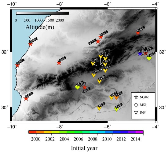
Figure 1.
Distribution of 10-min wind and wind gust observational sites. NCAxx (stars) stands for the sites provided by NCAR, METxx (diamonds) the data provided by Météo Maroc and IMPxx (inverted triangles) the data provided by the IMPETUS project. Color shading indicates the first year of the records at each site. “” denotes the identification label of each site (i.e., NCA, NCA, etc.)
These data altogether integrate an acceptable spatial coverage of observational data over the target region, consisting of 27 wind speed/wind gust series with records spanning the period 1999–2015. A summary of the wind data available for this study is outlined in Table S1 of the Supplementary Materials, where the description of the quality control (QC) procedure applied to the observations can be found.
2.2. High-Resolution Simulation over the Northwestern Sahara
The WRF (Weather Research and Forecasting Model) model [36,37] was used to generate a 12-year long (2002–2014) simulation at a horizontal resolution of 3 km. The length of the simulation allowed for capturing the intra- and inter-annual variability of the regional wind field, while the selected horizontal resolution was able to represent, with a high level of realism, the large heterogeneity of the terrain over the region of interest. Further details that help describe the set up of the model simulations can be found in Section 1.2 of the Supplementary Materials.
A comparison of the WRF simulated 10m wind with the same field from ERA-Interim reanalysis [38] is included in the Supplementary Materials. The comparison therein demonstrates that the higher resolution by the regional model relative to the wind field from the reanalysis largely benefits the estimation of the wind and wind maxima variability. Despite the smoothing effect—a feature that is expected in simulations compared to observations as a result of the averaging effect—it can be assumed that the model represents the wind variability with a high level of reliability and thus, it can be used to explore the spatial variability of high wind speeds as an idealized (model world) extension of the information provided by the observations.
3. Methodology
In this section, the theoretical frame and the experimental set up designed to estimate the wind and wind gust return values and their associated uncertainty are specified. A source of uncertainty in the estimation of extreme values and their recurrence arises from the selection of one single approach among the variety of methodological approaches in the literature. This type of uncertainty is systematically sampled in this section by exploring multiple options allowing an estimate of the sensitivity of results to the selection of the methodological choice. In a subsequent step, the uncertainty is constrained by applying several tests and filters in order to identify those reliable experiments that can be used to eventually obtain robust wind return levels.
3.1. Statistical Modeling of Extreme Winds
Several aspects as the type of family distribution, the methods to estimate the parameters of the distribution and the approaches to provide confidence intervals are discussed hereafter.
3.1.1. Probability Distributions of Extreme Values
The analysis of extreme events relies on the application of a statistical discipline, the Extreme Value Theory (EVT), to the available observed data [39]. There are two main families of probability distributions, i.e., the Block-Maxima and the Peak-Over-Threshold (POT) families (See the Supplementary Materials for further details about the EVT and the associated distributions).
The three Block-Maxima extreme value distributions are the Weibull, the Gumbel and the Fréchet distributions (see formulae in Section 2.1.1 of the Supplementary Materials). The differences in the asymptotic behavior of the tails of each family depend on the value of the corresponding parameters of the distribution (shape, location and scale parameters). The Weibull type (with , being the shape parameter) has a bounded right tail; thus, its upper end-point is finite. The Gumbel () and the Fréchet () types have instead unbounded or infinite right tails. Thus, each one has a different decay or convergence of the largest values in the sample to probability zero. In the case of the Gumbel distribution the decay is exponential, thus, it is faster than for the Fréchet case, that decays at polynomial pace.
In the first case, the distribution is termed light-tailed while in the second case it belongs to the heavy-tailed category. The behavior of the tails has strong implications on the probability that is assigned to the largest values of the population, and thus, it plays a fundamental role in the extrapolation of values out of the observed period. Therefore, the selection of the family type is a pivotal issue in the estimation of return values.
A common approach in pioneering applications of EVT consisted in adjusting the observations to one specific family, depending on expert knowledge of the data [39]. However, this approach suffered from two main drawbacks. On one hand, due to the scarcity of observations, expert knowledge is not usually ample enough to determine accurately the more adequate distribution, and therefore a more sophisticated method to determine the suitable distribution is opportune. Additionally, every hypothesis after the selection of a certain family is necessarily based upon such a selection, and an inadequate choice might, therefore, have a critical impact in the return level estimates of extreme events.
Additionally, a reformulation of the theory allows a generalization of the three types of families in a single model, the Generalized Extreme Value Distribution [40] (GEVD, Equation (4)). Thereupon, the procedure to fit the observed data dwells in making inferences solely about the shape parameter. By adjusting the shape parameter value with some numerical algorithm, the parent family is automatically and objectively determined without making any a priori judgments. This procedure is followed in this study. The protocols to obtain the parameters of the distribution will be detailed in the next paragraphs.
The Gumbel type has additionally been used to fit the observed wind extremes in this work; however, we avoided the use of Weibull and Fréchet probability distribution functions. Several arguments grant support to this decision. First, we are mostly interested in fast convergence to infinity. Therefore, distributions with finite upper limits, such as the Weibull type, are not considered since their bounded upper end-point s broadly imply that values larger than the observed ones are not expected.
Very slow convergence is associated with heavy-tailed families, such as the Fréchet one. This type is not frequently used in wind extremes analysis and is more typical in other fields, such as insurance and risk assessment and also in the telecommunications field [41]. This type of family shares the particularity of having infinite order moments, which complicates their use in, for instance, the application of certain goodness-of-fit tests later in this section.
The POT distribution families model the excesses of a variable over a certain threshold above which values are considered extremes. A collection of POT distributions is proposed in the theory. In this case, there are no restrictions about how many data belonging to one interval can be part of the sample. On the other hand, some criterion for the independence of the data should be considered when applying the POT scheme [42], that is, to establish a separation in time between the occurrence of two consecutive maxima to grant independence of events.
The necessary balance between the two criteria—the maxima threshold and independ-ence—suggests that higher thresholds require smaller gaps between the occurrence of events viceversa. Herein, the independence distance between two consecutive excesses is set as one day. Thus, extreme winds are considered independent from each other if they take place at least in consecutive days.
We are interested, as with the Block-Maxima, in the general formulation of the POT families, and thus we make use of the Generalized Pareto Distribution [43] (GPD), see the formula in Section 2.1.1 of the Supplementary Materials. The focus lies in the particular case with a light tail, that is, with exponential convergence to the infinite upper end-point. That is the case of the Exponential distribution, which is equivalent to the GPD with both shape () and location () parameters equal to zero.
Still, there is a third option, an alternative family of probability distributions, named the Point Process (PP), consisting in a combination of the two previous approaches—that is, the extreme values are modeled following the threshold excesses scheme; however, the theoretical distribution is expressed in terms of the block-maxima family type. In doing so, this generalization of the two main families has the advantages of making use of more data than in the Block-Maxima case, but at a time, it is independent on the threshold selection [44]. In this case, the occurrence of the extreme events is assumed to be Poisson distributed and the intensity of the event described by the Generalized Pareto Distribution. The parameters of the distribution are independent of the threshold and are equivalent to those of the GEVD [45].
Although additional possibilities could be also considered, as Sardeshmukh et al. [46], the large computational demand advised to included further choices in future studies. The final goal of each of the mathematical formalism applied is to characterize the wind speed and wind gust extremes by providing the quantiles that are expected to be exceeded with probability p once on average every return period . The latter is the definition of return level, that can be easily calculated making use of the parameters of the distribution (see formula in Equation (6), Section 2.1.2 of the Supplementary Materials).
3.1.2. Estimation of Distribution Parameters
There are also a variety of methods to estimate the distribution parameters. A classic approach is the Maximum Likelihood Estimation [40] (MLE) where the parameters that yield the most likely data, i.e., with higher probability to be consistent with the observations, are selected. Therefore, the method is based on maximizing the corresponding likelihood function.
There are additional options as for instance, the Generalized Maximum Likelihood Estimation method [47]. This variant has been applied in geophysical frameworks as for instance in the estimation of recurrence values of floods, rainfall, wind speeds etc. and is recommended for situations with small sample sizes.
Other usual option is the well-known L-Moment estimation [48]. The latter is considered a robust method to estimate the parameters in the presence of outliers in the sample. Another approach that deserves attention is the acknowledged Bayesian method [49], considered a powerful tool that can be more flexible and at least as robust as the extended MLE case in those situations where the classical methodology fails.
Its validity is based on the fact that it makes use of prior expert knowledge to improve estimations that are uniquely based on the observed data. Finally, the Probability Weighted Moments (PWM), is a very popular method in the context of hydrological extremes. It is mainly recognized because it eludes assigning large weights to very extreme observations avoiding so biases potentially due to outliers [50].
All methods present drawbacks and advantages and the motivation herein is to avoid the use of a single one and to explore the uncertainty space yielded by the use of different variants.
3.1.3. Definition of Extremes
One aspect that may contribute with additional uncertainty to the estimation of extremes recurrence is actually how the extreme values are defined. In both types of approach, Block-Maxima and POT distributions, the decisions made to define the maxima affects the bias-variance trade-off, that is, the choice of maxima to be fitted might influence how accurately the statistical model fits the empirical data (bias) and also how variable the estimate can be depending on the threshold/block selection (variance), respectively.
In this work, the uncertainty associated to the definition of maximum wind speed and maximum wind gust values herein is as well explored by allowing several options. Thus, in the case of the Block-Maxima, we estimate the return values for monthly, 6-monthly and annual maxima. In the case of POT distributions, extremes are defined as those values that exceed the 90th, 95th and 99th percentiles (P90, P95 and P99) of the wind speed series at each site. In doing so, we avoid sticking to a single definition of wind or wind gust extreme and we explore what is the impact of the selection of a particular definition of wind extreme.
3.1.4. Confidence Intervals and Goodness-of-Fit Tests
The classic approach when fitting observed data to theoretical distributions is to provide the standard error or a confidence interval to evaluate how suitably the empirical data fit the selected theoretical distribution. The resulting confidence intervals eventually inform us about the statistical confidence. Two methodologies, the standard Normal [51] and the Bootstrap, are explored in the present study in order to evaluate the impact of selecting a certain error estimator [52].
Nevertheless, the uncertainty estimate provided by a single confidence interval should be regarded as the lower bound of the uncertainty, since they just inform about the influence of selecting a certain probability distribution while, as explained above, the sources of error are more diverse. Thus, a confidence interval arising solely from the standard error estimation might be to a large extent an insufficient estimate of the uncertainty associated to the return level of an extreme event. A comprehensive sensitivity analysis that makes use of multiple methodological variants is considered the most robust evaluation of the reliability of the extreme values estimates. Based on that, a probability estimation associated to the return levels is determined. This is described in the next subsection.
It is not unusual that a particular method might fulfill one test but fail another. Thus, the question whether different goodness-of-fit (GOF) tests are sensitive to specific aspects of the distribution seems pertinent. To avoid focusing on any particular feature of the distribution and to confer robustness to the fits by allowing only those cases that succeed more than one test, a pool of five GOF tests was applied to each fit. They are specified in Table 1, which summarizes all experimental variants considered. It also indicates that the experiments were applied to the observational data and to the high resolution regional simulation as well.

Table 1.
Summary of experiments. All methodological variants applied in the first part of this work are indicated. Every one of these configurations is tested over each time series within the observational wind/wind gust data set.
Nevertheless, the resulting return levels provided in Section 4.2 are based exclusively upon the observations. Table 1 indicates that wind return levels were estimated for two different variables, the daily maximum 10-min wind averages and daily maximum wind gust. The total number of experiments, considering all possible combinations of methodological choices in Table 1 at all locations where there are available observations is ca. 10,000.
The experiments designed in this work shape a methodological sensitivity analysis of the wind return level estimation. The multiple experimental configurations tested allows to expand the uncertainty space and provides a quantification of the methodological variance. However, not all configurations applied are expected to provide reliable estimations of the wind extremes recurrence. Therefore, in a second phase, a strategy that identifies the cases that cannot be considered reliable becomes necessary. In doing so, we provide constraints to the uncertainty by selecting only the best suited experiments to infer the wind return level estimates. The approach designed to filter out the less reliable experiments is described in the following section.
3.2. Constraining the Methodological Uncertainty
Once the observed wind series were adjusted using a particular configuration (see Table 1), the return levels are estimated as the quantiles of the distribution. There is no standard procedure to assess the quality of the estimated return levels in the literature The filters or assessments applied herein to determine the trustworthiness of each configuration are based on evaluating the ability of the distribution to represent the observed data [40].
The latter implies that, if a specific choice suitably fits the observed wind extremes, then it is assumed that the corresponding configuration is appropriate to extrapolate the extremes occurrence out of the observational period. We used a pool of sequential filters to ensure that the remaining experiments are reliable in a sense to be defined in the following paragraphs. In this way, the uncertainty expanded by applying multiple methods in the former section can be constrained.
The competence of the statistical methods applied herein to fit the observed data was verified in this study by means of a set of different tests and model diagnostics (MD). These involve metrics for how the observed extremes occurrence fits the theoretical probability distributions. As the first model diagnostic (MD1), five different GOF tests are applied to each one of the configurations explored (Table 1) The number of tests that each experiment should succeed to positively accomplish in MD1 is determined on the basis of the relative frequency of the amount of GOF tests that are surpassed by the pool of experiments carried out. A histogram of the frequency of GOF tests successes is represented in Section 4.1 to help define the threshold that indicates which configurations should not be considered reliable.
After this filter is applied to the pool of configurations, a confirmation test verifying that the experiments rejected should be indeed considered unreliable or invalid is advisable. With this additional check (hereafter the confirmation check), it can be assured that the filter does not disqualify any valid experiment. However, this method does not guarantee that invalid cases survive until the very last filter (MD) is applied, when the surviving experiments are also individually scrutinized, so that no unreliable cases are kept for the final return level estimation step.
An experiment is considered objectively invalid if the fitting does not appropriately represent the observations. In order to decide if the configuration fails in modeling the observed extremes, the Return Level plot is used. In this classical representation, the return level estimates for each return period are shown accompanied by the corresponding confidence interval estimates. The empirical return levels (observed extreme winds) are also represented together with the estimated return values.
If there are n points (e.g., n yearly maxima) in an experiment, the highest value corresponds to the empirical n-year quantile, the second maxima is the (n-1)-year empirical quantile and so on [40]. Thus, if the fit is suitable, the observations compare well with the estimations for return periods equal or shorter to the observational period (in our case the observational period ranges between 4 and 15 years). To compare well with observations, the empirical points should be comprised within the corresponding 95th confidence interval. Otherwise, the experiment is rejected. The empirical return levels are calculated by interpolating the observed extremes in the corresponding estimated return level (solid black) line.
Figure 2 illustrates the latter for one random experiment as an example. In this plot, the estimated return levels are given by the solid black line, and the dashed lines are indicative of the confidence intervals (40th–60th, 30th–70th, 20th–80th, 10th–90th and 5th–95th). Several empirical return levels (black points) fall outside the 95th confidence interval indicated by the upper- and lowermost dashed lines (dashed red). In such a case, the configuration is cataloged as invalid. Otherwise, if all empirical values lie within the 5th–95th confidence interval, the experiment is considered valid. This check is performed after each single filter.
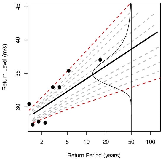
Figure 2.
Return level–return period plot of a random configuration as an example. The estimated return levels are given by the solid black line, and the dashed lines represent the confidence intervals (40th–60th, 30th–70th, 20th–80th, 10th–90th and 5th–95th, in red). The empirical return levels (black points) are also represented.The thin black curve indicates the shape of the corresponding probability density function calculated based on the distribution of confidence intervals.
The next filter denoted as MD2 considers that the estimated extreme wind values must range within a realistic interval. Therefore, all experiments that provide wind return levels out of the range [0 ms, 112 ms] considered in the scientific literature as physical limits for wind velocities [63], are then rated as not realistic, and the corresponding experiment is discarded. This test was only applied to the experiments dealing with 10-min wind speed, since higher wind gust are indeed plausible.
The following paragraphs describe a sequence of four additional diagnostics. After each of them, the confirmation check corresponding diagnostic is also applied. The diagnostics are based on the quantile–quantile (q-q) plot, the histogram-density function (h-h) plot, the probability–probability (p-p) plot and the return level-return period (RL) plot [40]. They all are oriented to compare the experimental and the theoretical distributions. Since each diagnostic helps in rejecting invalid cases, the following filter is applied only to the remaining experiments.
The model diagnostic based on the q-q plot (MD3) compares the quantiles of the observed population to those from the theoretical distribution that fits the observations (for further details see Figure S7 in Section 2.1.2 of the Supplementary Materials). The fit is considered suitable if the observed vs. the theoretical quantiles yields a straight one-to-one line. A typical “S”-shape in these plots suggests that either one of the distributions is more skewed or has heavier tails than the other. Therefore, convergence to the upper end-point might not be robust. In this work, we consider the skewness as a strong indicative of a poor fit.
To allow an automatic calculation of the skewness, the “S” shape is characterized by a measure of the distance of the values in the q-q dispersion plot to the line (perfect-prognosis). The metric used in this case (and also in the next diagnostics) as a measure of the distance is the root mean of the squared distances, and therefore the statistic employed, is the Root Mean Squared Error (RMSE). Larger RMSEs imply less reliable fits, while smaller distances suggests a better adjustment to the observed wind data. Therefore, an RMSE value above which the corresponding configurations are considered unreliable needs to be determined. In order to decide this RMSE threshold above which the experiments are excluded, the RMSE values from all experiments are represented in a dispersion diagram against the corresponding estimated wind return levels.
This provides a first understanding about how abnormally high the RMSE values can be. Additionally, to help establish the RMSE threshold, the relative frequency of the all RMSE values after applying the qq-test is calculated and represented as a histogram. Those values that lie in the upper tail of the frequency distribution are considered abnormally high. The selection of the limit value above which the experiments are rejected is subject to the posterior application of the confirmation check. Thus, if valid cases result as rejected, the selection of the RMSE threshold is reexamined so that no reliable cases are excluded. The same strategy is implemented for each of the filters considered.
An additional aspect that might enlighten when a RMSE value can be abnormally high and help therefore in the selection of a threshold value is whether a relation between the fit error (RMSE) and the magnitude of the associated return value can be detected. If a plausible linearity between the return levels and the RMSE values is identified, this is indicative of the larger return levels being associated with larger RMSEs. This would be an undesirable feature since it would imply that larger expected extreme values are not realistic but an artifact of arising from a poor fit and these experiments should be considered as potential candidates to be rejected.
Finally, a last aspect to be considered in order to determine an RMSE threshold. Very wide confidence intervals, particularly for long return periods, could be indicative of some kind of convergence problem in the fitting. These cases are suspicious of being the result of a poor fit. Thus, if the confidence intervals are comparatively wider relative to the bulk of experiments, it can be broadly considered suggestive of an inadequate fit of the distribution to the observed values.
Thus, an indirect measure of the suitability of a distribution to model the observed extreme values is whether its associated confidence interval is outstandingly wide, relative to the sample population. A tendency to wider upper than lower confidence intervals was observed in most of the fittings (not shown). Thus, only the upper bound width of the confidence interval was represented in the right y-axis of the corresponding RL-RMSE dispersion diagram to identify fit inadequacy. These steps (RL-RMSE diagram and the histograms of relative frequencies of the RMSE values to decide a RMSE rejection limit) are repeated after each model diagnostic.
The following model diagnostic, MD4, is based on the h-h plot (see Figure S7b in Section 2.1.2 of the Supplementary Materials). In this case, the empirical histogram, as an estimate of the probability density function, is compared with the theoretical function and a measure of how close they are to each other is provided by the RMSE values calculated between the empirical and adjusted probabilities. The corresponding RL-RMSE diagram as well as the histogram of the relative frequencies of the RMSEs are represented as in MD3 to determine a threshold to reject potential invalid cases. After that, the confirmation check is again applied to detect whether valid cases were rejected.
The fifth model diagnostic (MD5) calculates the distance between the empirical and the theoretical distributions as the RMSEs from the the p-p diagram (see Figure S7c in Section 2.1.2 of the Supplementary Materials), which is equivalent to the previous ones, but it represents the pairs of the empirical versus theoretical probabilities.
The last model diagnostic (MD6) is based on the RL plot (recall Figure 2 in this section and see as well Figure S7d in Section 2.1.2 of the Supplementary Materials) and implies the identification of anomalously wide confidence intervals. In this case, the dispersion diagram is based on an “RL-Upper confidence interval width” instead. Experiments showing anomalously wide confidence intervals are withdrawn in this part of the analysis. Recall that again ‘anomalous’ is define within a frequentist frame, that is, comparatively with the rest of values from all remaining experiments. The dispersion diagrams as well as the histogram of relative frequencies of the upper confidence interval widths are used in this step as before.
The confirmation check was applied after each filter, and those experiments whose empirical points (observed wind speeds) fall out the 95th confidence interval from its corresponding fit are rejected. Based on this test it can be confirmed that no valid or reliable cases are rejected. In addition, the very last step of the procedure involves a new confirmation check applied to all remaining experiments after the pool of filters described above to ensure that no invalid experiments survived the filters.
Additionally, a probabilistic representation of return level estimates is provided in the results section. It is based on determining the mixed or combined probability [64] as a combination of the individual probability distribution functions (PDFs) at each site. The individual PDFs are estimated by calculating an array of quantiles. They correspond to the accumulated frequencies of the individual PDFs (a random example is represented in Figure 2). Once the individual PDFs were calculated, each one corresponding to one successful experiment at a specific site, the combined PDF is obtained as the normalized average of each site PDFs.
In doing so, we obtain the probability densities of the combined PDF from which different statistics can be drawn. We estimate the median as the most probable return value from the combined PDF at each site for every return period from 10 to 100 years. The upper and lower confidence limits are represented therefore by the probability densities, the higher the confidence level selected, the lower the probability of occurrence of an extreme wind larger than the corresponding return level. Thus, we represent herein the 5th–95th confidence intervals.
The methodology exposed represents the best guess of a semi-automatic quality control applied to an extensive amount of configurations, which constitutes an exhaustive sensitive analysis of the variety of methodological approaches.
4. Results
This section illustrates first the results of the evaluation of the reliability of the multiple experiments from Table 1 (Section 4.1) as narrated in Section 3.2. The final estimates of wind speed and wind gust return levels for return periods up to 100 years together with an estimate of their uncertainty are presented in Section 4.2. Finally, simulated wind return level maps for 50- and 100-years return periods are presented in Section 4.3.
4.1. Methodological Sensitivity Analysis of Wind Return Levels
The number of succeeding GOF tests (MD1) are represented in Figure 3 where the relative frequency refers to the total number of experiments before applying any test. Figure 3 shows that approximately one third of the experiments surpass the five tests in Table 1, ca. 27% do not pass any of them and approximately a third of the total number of configurations applied pass between one and four GOF tests. Thus, Figure 3 demonstrates that the number of fits that succeeded more than one GOF test is relatively high (ca. 75%).
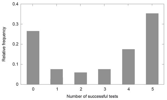
Figure 3.
Histogram of successful goodness-of-fit tests. The relative frequency of the amount of experiments that surpass a certain number of tests (up to five) is calculated with respect to the total number of experiments initially implemented.
In order to explore which methodological options tend to succeed the tests, the histograms in Figure 4 are segregated according to the different methodological variants. In general, it can be appreciated that there are no options in the definition of the wind extremes (Max. Def. in Figure 4) that clearly demonstrate a higher rate of successful tests than others.
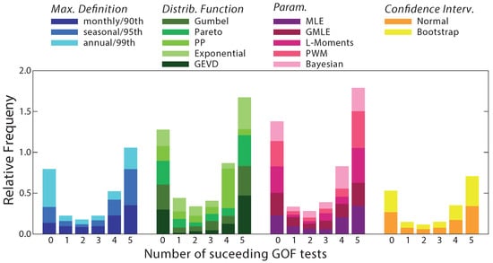
Figure 4.
Histograms of successful goodness-of-fit tests segregated according to the various methodological options (see colors in legend). Max. Def., indicates the criterion followed to define the wind extremes, depending on whether the corresponding family distribution is Block-Maxima or POT (see Table 1 in Section 3.1); Distrib. Function relates to the family distribution; Param. stems for the parameter estimation method; finally Confidence Interv. indicates the methodology to estimate confidence interval within each individual experiment.
It is noteworthy, however, that, among the group of experiments failing all five GOF tests, we find a large number of experiments where the amount of data is small, for instance those cases where the wind/wind gust extremes are defined as the annual maximum or defined as those values above the P99. This is an expected feature, as one of the main obstacles for an acceptable fit is the shortage of the data. MD1 provides evidence of how critical the length of the observational sample is.
In the case of the different family distributions (Distrib. Function, second group of histograms in Figure 4), it is noticeable that the PP family shows a small number of cases with five successful tests, while the Exponential distribution presents larger frequency of successes. The opposite is true if the frequencies with four positive tests are analyzed. However, these features do not necessarily imply a preference of any of the families of distributions to succeed more tests. The same applies to the parameter estimation methods (Param in Figure 4) and the approach followed to obtain the confidence interval.
Figure 3 and Figure 4 demonstrate that making inferences about extreme events on the basis of a single test is arguably less trustworthy, and the use of more GOF tests help increasing the confidence on the remaining experiments. Thus, we propose that the requisite to consider a fit acceptable is that it succeeds at least two tests.
After rejecting those experiments that turned out in estimated return levels larger that 112 ms (MD2), the filter MD3 on the basis of the q-q plots is applied. Figure 5a shows the corresponding scatter diagram of the wind return levels for a return period of 50 years (as an example) vs. the RMSE values (RL-RMSE diagram) obtained from the q-q plots for all experiments that succeeded previous filters MD1 and MD2. Comparable results are obtained for return periods corresponding to 80 and 100 years. The upper 95th confidence limit of each individual experiment can be identified by the color scale. Values above 1 ms are seemingly outliers with respect to the cloud of points.
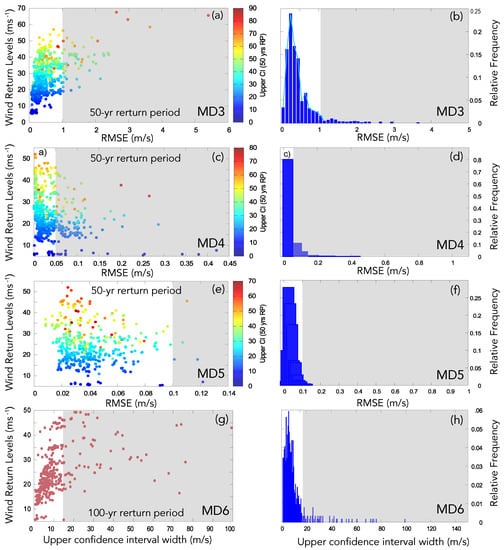
Figure 5.
Sequential model diagnostics. Left. 50-year RMSE values calculated at all locations and for all remaining experiments from the previous test as (a) the difference between the observed and the theoretical quantiles (q-q plot), (c) the difference between empirical and theoretical density functions (h-h plot), (e) the difference between empirical and theoretical probabilities (p-p plot), the color indicates the upper 95th confidence limit of the corresponding return value before the filter is applied; (g) the wind return levels against the confidence interval width for a return period of 100 years from the evaluation in MD5. Right. (b,d,f,h): histograms of relative frequencies (with respect to the number or remaining experiments from each previous test) of RMSE values before the corresponding filter is applied. Grey shadow in all panels stand for the RMSE values of experiments that are filtered out in each step.
The diagram in Figure 5a also indicates that some of the largest RMSE values present wider upper confidence intervals (yellow-orange-red, see points color legend in Figure 5b), as expected. These cases should be considered as doubtful fits as commented in Section 3.2. Figure 5a demonstrates as well the dependence of the fit errors (RMSEs) upon the estimated wind return values. The scatter diagram suggests that the highest wind return levels go well along with the highest RMSE values, a relation that could indicate some sort of bias in the estimates of extreme values, suggesting a link between the highest wind values estimated and the quality of the fit.
As explained above, in order to determine a RMSE threshold above which the experiments should be checked and excluded if appropriate, the relative frequency of the RMSE values is additionally represented as a histogram in Figure 5b. A decay of the relative frequency in the histogram is indicative of abnormally high RMSE values. Thus, a potential cutting point can be inferred from the decay of the tail of the histogram. Based on both plots (Figure 5a,b), the threshold is set to 1.0 ms since the vast majority of RMSE values without an outstandingly large upper confidence limit are below that value.
All experiments that do not fulfill this requisite are disregarded. In doing so, most of the reddish dots with larger upper confidence intervals are eliminated in this step. After removing the failed experiments, there is no longer an explicit relation between the magnitude of the return level estimates and their 95th confidence intervals width or the associated the RMSE values (not shown). The threshold used in this filter was compared to those threshold that would have resulted if using the 80-year and 100-year return values instead to check their robustness, showing consistency in the three cases. All rejected cases are subjected to the confirmation test in order to exclude the possibility that potentially valid cases were eliminated.
Figure 5c,d illustrate the decision-making for rejecting those experiments with higher RMSE values in the h-h plot (MD4) also for a return period of 50 years, as an example. We additionally used 80-year and 100-year return periods in this analysis (not shown) demonstrating coherence with the threshold proposed in this test. Similar comments about the scatter diagram as in Figure 5a can be brought here. However, a direct relation between the higher RMSE values and higher wind return levels estimates is now less evident than in the previous case as a consequence of the correction already performed in MD3. The histogram in the right panel helped identifying that all RMSEs greater than 0.05 ms are potential candidates to be rejected. After removing these ill-suited experiments no actual dependence of the RMSEs with the wind return values was detected (not shown).
The next model diagnostic is MD5 based on the p-p plot. The corresponding return levels-RMSE dispersion diagram and the histogram of RMSEs relative frequencies are represented in Figure 5e,f, respectively. The scatter diagram suggests that a very small number of experiments are candidates to be rejected in this step. A judgement that can be identically inferred from the histogram in Figure 5f. In this step, the dispersion diagram and the histogram accordingly suggest to disregard only those experiments with an RMSE > 0.1 ms.
No clear evidence of any relation between the higher return values and the largest RMSEs can be identified in Figure 5e after the filter is applied. The scatter diagram shows, however, a certain relation between the highest return levels and the higher upper confidence limits. This particularity can be, however, also suggestive of larger uncertainty associated with the estimation of the most extreme values, showing, thus, the corresponding fit for wider confidence intervals.
Figure 5g presents the estimated wind return levels against the upper confidence interval width for a return period of 100 years for all remaining experiments from previous steps. As commented in the previous step, the confidence intervals are by default wider for higher return periods, since the uncertainty seems to increase as the probability of the extremes decreases. Therefore, the selection of a longer return period, with potentially higher return levels, aims at ease the detection of comparatively too wide intervals that might might be indicative of very large uncertainty and therefore doubtful fits. In view of the histograms and scatter plots in Figure 5g,h, the decision of disregarding all experiments with a confidence interval width higher than 16.0 ms was made.
This value represents the cutting threshold above which the RMSEs are less frequent and more sparsely distributed (see histogram in Figure 5h). The confirmation check was again applied over the pool of rejected cases to detect whether well suited experiments could have been eliminated.
After applying all filters, an automatized screening implemented over the remaining configurations instead was performed in order to detect if any of the surviving experiments presented empirical points out of the confidence interval, implying that ill-posed configurations have surpassed all filters above. No cases were eliminated in this last step.
A total of 40% of the total initial experiments succeeded the sequence of filters applied. The evaluations performed so far constitute an exhaustive analysis of the quality of the fits aimed at identifying which experiments are not well suited to adequately represent the empirical distribution of observed wind and wind gust and therefore are not appropriate to provide wind return estimates.
We explore what are the methodological options that predominantly passed the filters. This is represented in Figure 6. The panels therein represent the proportion of successful experiments for each variant within the ensemble of methodological alternatives used. Figure 6a shows to a certain degree a preference for the GEVD type of distributions. The latter is an expected feature as this distribution is the more flexible case within the Block-Maxima type. This allows for self estimations of the parameters of the distribution (in the case of Gumbel, the shape parameter is forced to equal zero, see Section 3.1.)
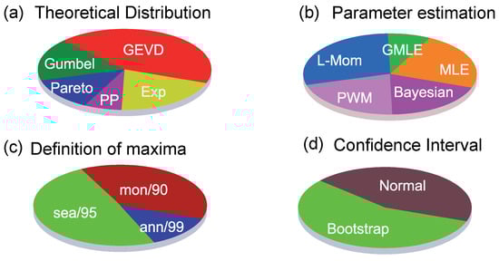
Figure 6.
Pie-plots representing the rate of successful experiments for each methodological variant: the respective proportion of remaining experiments after applying filters from MD1 to MD6 according to (a) the corresponding family distribution, (b) the parameters estimation method, (c) the criterion to select the wind extremes and (d) the method to estimate the confidence intervals.
In addition, the literature suggests that the GEVD presents higher chances to provide reliable fits in situations with scarcity of data [40]. The PP distribution shows the smallest amount of successful experiments, and, among the other three cases, a similar partitioning of experiments can be noticed. It can be said that in the succeeding rates there is a representation of all families that support the initial argument of testing all of them in this study.
The partition of experiments according to the parameters estimation is not particularly biased towards any of the options in Figure 6b. Relative to the definition of extremes, the less successful cases are the annual maxima as expected, since the shortage of values in these experiments hampers a good fit (Figure 6c). Finally, both methods to estimate the confidence intervals are equiprobable (Figure 6d). Therefore, in view of the tendency of the experiments to broadly distribute homogeneously among the methodological variants after all filters were applied, it seems reasonable to argue that the quality of the fits do not strongly depend on any specific experimental configuration, supporting; thus, the approach presented herein based on exploring a variety configurations to expand first and constraining after the uncertainty space.
The question of whether some variants are prone to produce larger/smaller return values than others seems also interesting. The 10-min wind and wind gust 50-year return levels are represented as a function of the corresponding theoretical distribution in Figure 7 for all successful experiments. The color indicates the q-q RMSE values, and the size of the circles represents the upper confidence limit at the 95th level. Hence, the larger the confidence interval, the larger the circle. We are interested in two types of questions. Do the diagnostics (q-q RMSE values in this case as an example) of the remaining experiments reveal a dependence on any specific distribution?
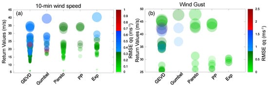
Figure 7.
The 50-year 10-min wind (a) and wind gust (b) return values segregated according to the corresponding family distribution and as a function of the RMSE calculated from the q-q plot.
Figure 7a,b illustrates that both smaller (greenish) and larger (bluish and reddish) RMSE values are obtained for all theoretical distributions used. The same applies if the RMSE values from the other diagnostic plots are used instead (not shown). Therefore, it can be argued that none of the probability distributions employed in the analysis produces larger RMSE values compared to the rest. Additionally, we are interested in examining whether the largest wind return values depend on any particular probability distribution. Figure 7a,b indicate that there is no apparent arrangement of the return level magnitude according to the family distribution. Therefore, how extreme the expected wind and wind gust return values are seems to prove independence on the selection of the theoretical distribution.
On the other hand, the size of the circles increases as the wind return values increase, more noticeable in the case of the 10-min wind (left) but also for the wind gust (right), which can be considered again an expected feature since as explained before, it implies that the larger the expected extreme wind, the larger the associated uncertainty.
4.2. Wind and Wind Gust Return Level Estimates over Northwestern Sahara and High Atlas
This section is dedicated to present the resulting estimates of wind and wind gust return levels that can be expected for return periods up to 100 years over the region under study as a result of the methodological sensitivity analysis performed in the previous section. We first provide a classic representation of estimates based on their frequency of occurrence and a rough notion of the associated uncertainty based on the spread of the resulting values. Later, in this section, we provide as well a more comprehensive probabilistic frame to represent the estimates of wind speed and wind gust return values together with their corresponding probability as a measure of uncertainty.
Figure 8a shows the 50-year 10-min estimated wind return levels and the corresponding confidence intervals at each location for the experiments that succeeded only the first two tests (MD1 y MD2, recall Section 3.2), after the largest unphysical estimates are removed. The same is represented in Figure 8c for the wind gust. The green box-whiskers represent the frequency distribution of wind return levels, while the red (blue) boxes and whiskers represent the same but for their corresponding upper 95% (lower 5%) confidence limits of the successful experiments after MD2.
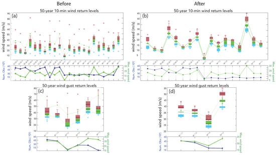
Figure 8.
Top (a,b): box-whiskers plots of 50-year 10-min wind return values at each site within the dataset for experiments that succeeded tests MD1 and MD2 (left) and after all filters (MD1–MD6) were applied (right); green boxes represent the frequency distribution of the 10-min wind return levels over all experiments; the 10th, 25th, 50th, 75th and 90th percentiles are indicated with whiskers; the 50th percentile (median) is highlighted with a dark green horizontal line in each box; red (blue) box-whiskers represent the frequency distribution of the upper 95% (lower 5%) confidence limits of each successful experiment; red (blue) dots in the top panel stand for the maximum (minimum) values of the upper (lower) confidence intervals. The time series in the panels below represent the number of observations (dark blue) and maximum wind speed (green) recorded at the corresponding site represented in the left and right y axes, respectively. Note the different scales in the right and the left panels. Bottom (c,d): As above but for the wind gust.
Maximum (minimum) upper (lower) values are also represented with red (blue) dots. The medians are highlighted with a horizontal line at each box. In some cases the median is close to the center of the green box (e.g., IMP08). However, the cases where the median is biased towards the lower extreme of the box are apparently more numerous, thus, implying some positive skewness of the frequency distribution of the return values. This particularity can be understood if a probability distribution is represented instead, then a long upper tail of the distribution would be noticeable.
Upper confidence interval bounds show generally much more spread than the lower ones (red and blue box-whiskers plots, respectively) implying a tendency to wider upper confidence ranges, which is indicative of larger uncertainty associated to larger wind and wind gust return values as already explained. It is also striking that for instance the maximum upper confidence limit at NCA05 (Figure 8a) is larger than the corresponding values of wind gust (Figure 8c), indicative of some level of inconsistency that is corrected later (Section 4.1). Larger wind return values and upper confidence limits are related to larger mean winds (green time series in the panels below).
The 10-min wind speed (wind gust) return levels for a 50-year return period, after applying all remaining filters (MD3 to MD6) are shown in Figure 8b,d. The reduction of the range of wind return values in both, the 10-min wind and the wind gust with respect to Figure 8a,b are noteworthy. Upper limit values above 80 ms could be found before, whereas now the maximum upper 95th confidence limit over the remaining locations and experiments is around 45 ms (56 ms) for the 10-min wind speed (wind gust). Therefore, before the application of all MDs that guarantee the quality of the fits, poor fits could potentially result in higher wind return values and/or mostly wider confidence intervals due to larger uncertainty. Such a relation no longer holds after constraining the range of reliable experiments.
Figure 8b,d demonstrates that some sites were completely withdrawn after the sequence of evaluations since all experiment configurations were rejected due to their ill-suited fits to the observations. In most cases, where the theoretical distributions were found not suitable to fit the observations, a convergence problem due to the scarcity of data was involved. This is illustrated by the blue time series below each panel representing the size of the sample available at each location. Some examples of the latter are NCA17 or IMP09 (Figure 8a,c) with 10-min wind observations or IMP02 and IMP09 (see Figure 8b,d) with wind gust records. Therefore, from the initial pool of 27 observational series, only 21 series succeeded the complete sequence of filters.
The resulting wind return level estimates evidence of relatively small dispersions at each location in comparison to the estimates before the filters at some of the sites. This is true particularly at the NCAR locations. The latter implies that the remainder experiments agree reasonably well in the estimations they provide at these locations. The latter also holds for the dispersion of the upper and lower 95th confidence limits. After the tests, the maximum confidence limits (red dots) are generally closer to the 90th percentile than in Figure 8a,c.
This additionally supports the argument of less dispersion and skewness in the final estimates, and therefore more agreement among the remaining configurations after the filters. The estimates of the 50-year 10-min wind return values are in general below the 30 ms except the IMP07 site located at a high altitude over the Atlas. In the case of the wind gust, the four remaining sites show sensible differences in their estimates of the 50-year return values in Figure 8d.
We provide, hereafter, a probabilistic representation of return level estimates based on the mixed or combined probability. As said in Section 3.2, we calculate an array of quantiles instead of only the 5th and 95th percentiles as in Figure 8. The combined PDFs of the most windy sites, for both the 10-min wind speed and wind gust return levels for various return periods between 20 and 100 years are presented in Figure 9 as an example.
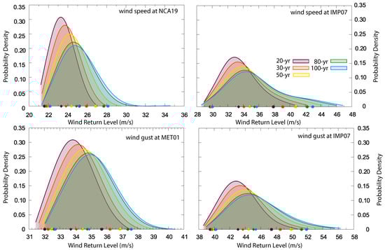
Figure 9.
Combined PDFs of the wind return levels for 20-, 30-, 50-, 80- and 100-year return periods (see legend for colors) at some of the sites within the database as an example. Each PDF is built upon the experiments that fulfill the pool of filters applied to the ca. 10,000 initial experiments. Symbols indicate the 5th and 95th percentiles (circles) and the median (diamonds) of each distribution.
The percentiles 5th and 95th (circles) and the median (diamonds) are indicated in the PDFs, where the color refers to the corresponding return period. Specially for the longer return periods, the PDFs are positively skewed, which was already expected since it is typical of the distributions describing extreme values. The PDFs become more platykurtic as the return period increases.
The PDFs of the 10-min wind and wind gust return levels in NCA19 and MET01 (both series are co-located) are more peaked (leptokurtic) than those at IMP07, located over the High Atlas. Therefore, the kurtosis of the PDFs does not necessarily depend on whether the return levels are calculated for the wind speed or the wind gust but on the particular features of the wind at a specific site, illustrating the fundamental role of the spatial variability in the probability of occurrence of extreme wind events.
In the case of the 10-min wind speed, the median of the distribution is 24 ms (25 ms) and 35 ms (37 ms) at NCA19 and IMP07, respectively, for a 50-year (100-year) return period, while in the case of the wind gust the same locations might expect wind return levels above 34 ms (35 ms) and 44 ms (45 ms), respectively, for the same return periods. If we consider the 95th percentile of the distribution (circles), return values for a 50-year (100-year) return period of 27 ms (28 ms) at NCA19 and 41 ms (43 ms) at IMP07 are found in the case of the wind speed, while for the wind gust 37 ms (38 ms) at MET01 and 50 ms (52 ms) at IMP07 are plausible. It is noticeable that the return values of the 50-year levels are not sensibly larger compared to those for a 100-year return period. Therefore, a monotonic growth of the magnitude of the wind return levels with the return period seems apparent.
The map of wind return level estimates for the 50-year return period in Figure 10 provides some insight into the spatial variability of the wind sped and wind gust return estimates. The 5th percentile (inner circle for 10-min wind and inner star for wind gust), the median (middle) and the 95th percentile (outer) of the probability distribution of the 10-min wind speed and wind gust return values (from Figure 9) are represented with concentric symbols at each site within the dataset.
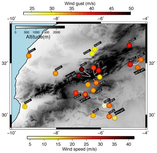
Figure 10.
50-year return values of the 10-min wind speed (circles) and wind gust (stars) for all sites within the observational dataset (note there is a different color scale for each variable). The color of the mid symbols represents the median of the 50-year return values. Outer (inner) circles are illustrative of the 95th (5th) percentiles of the respective combined probabilities from the successful experiments at each site. Gray shading stands for the topography of the region.
Larger return values are expected over mountainous terrain at the higher altitude locations. The downstream flows in the Ouarzazate Valley can be associated with higher winds and therefore larger wind return values are also visible over this area. Smaller values upstream the High Atlas mountains and downstream to the south are noticeable.
The next section illustrates how the simulated return levels serve to the purpose of making further inferences about the spatial variability of the extreme winds over the broad area of the High Atlas and northwestern Sahara.
4.3. Simulated Wind Return Level Maps
This section shows that model evidence can help in providing a description of the spatial variability of the wind return levels over the area under study with greater detail than the observations. This analysis lean on the realism of the WRF model simulation described in Section 2.2 in reproducing the mean wind field and some characteristics of the temporal occurrence of extreme wind values. An accurate representation of the observed features by the model would be desirable; however, biases are also expected and can be potentially improved in future model experiments.
Additionally, the smoothing effect due to the unresolved processes in the simulation hampers the comparison of observed and simulated wind extremes. Therefore, the model is used solely to provide a frame that may be of use in the interpretation of observations but not to provide final estimates based on the model simulation.
A comparison between the wind return values from the observations and from the simulation is performed, that serves as an evaluation of the ability of the simulation to provide estimates of return values after the statistical methods described in Section 3.1 are applied to the simulated data. The comparison of the return levels calculated from observations and from the modeled wind field requires that the simulation mimics the observations in time and space. This implies that the comparison focuses on the wind series from those model grid-points that are co-located with the observations. A temporal mask needs to be applied by placing a missing value in the simulation at the time-steps where the observations are also missing. Otherwise differences between observations and simulations could be due to the different sampling.
The approach is based on applying to the simulated wind only those experimental configurations that succeeded at each observational site to the series at the simulation nearest grid point. Once the fits and all subsequent filters are applied, the wind return levels from the simulated wind are obtained identically as were obtained in Section 4.1 and Section 4.2. Thus, the different experiments at each grid point co-located with the observational sites allow the estimation of a PDF from which the median of the distribution as the best-estimate and the confidence intervals can be extrapolated. The comparison between the observed and the simulated wind return levels can only be done in terms of the 10-min wind speed. It cannot be expected that the model reproduces processes at the turbulent scale that contribute to a great extent to the wind gusts. Therefore, the daily maximum wind from simulations is only compared to the 10-min wind from observations.
The normalized PDF of the wind return values calculated from both observations (in red) and simulations (in blue) are represented in Figure 11 for NCA06, IMP11 and NCA19, as an example. They represent two different situations where the simulated and observed wind return values are very close to each other, in the case of NCA06 and IMP11. Not only are the medians (diamonds in Figure 11) of the corresponding PDFs very close to each other, also the confidence intervals provided by the 5th and 95th percentiles (circles) demonstrate a very good agreement in both cases.
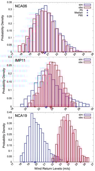
Figure 11.
PDF of wind return values for a 50-year return period obtained from observations in red and simulated wind in blue at the NCA06 (top), IMP11 (middle) and NCA19 (bottom) sites. The 5th and 95th percentiles (circles), and the median (diamonds) are also represented.
On the other hand, at the NCA19 site, a shift of the simulated PDF to lower wind values is evident; therefore, at this site wind return values provided by simulations are smaller than those provided by observations. This bias between observed and simulated wind return levels is smaller than 4 ms (2 ms on average) at the NCA19 site (note the different scales at each site). In spite of the previous, the shapes of both simulated and observed distributions are very similar in the examples presented in Figure 11 and, in general, in all sites where observed and simulated PDFs can be compared (not shown). Since, the model return levels seem to be in a reasonable agreement with those from the observations, an exploration of the spatial variability of the wind return levels from the model pseudo-reality seems plausible.
The wind return values for 50- and 100-year return periods are provided for the simulated wind during the whole period of simulation. Return level maps are valuable to explore the spatial variability of high wind speeds [58] and, therefore, to identify the regions that are more exposed to extreme winds and how this might depend on the return period selected. With this aim, the successful experiments from Section 4.1) were applied to the simulated wind time series at each grid point within the sub-domain D4 (see Figure 12), inside the domain D3 of the simulation. The ideal situation would involve to extend the analysis to all grid points within the innermost D3 domain. However, the computational constraints imposed the use of a smaller domain that still captures the area of interest.
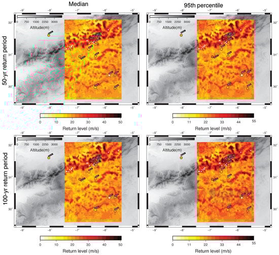
Figure 12.
Maps of simulated wind return levels for a 50-year (top) and 100-year (bottom) return periods obtained from the regional model unmasked simulation for a region within the D3 domain (sub-domain D4). The median (left) and the 95th percentiles (right) from the mixed PDF at every grid-point were represented. Return levels calculated from observations are also represented (circles) for comparison. Note that only those observational sites with remaining successful experiments from the sensitivity analysis in Section 4.1 are included in these maps.
The successful experimental configurations at the closest observational site was applied to the simulated daily maximum wind at each grid point. The combined PDF was calculated as was done for the observations at every grid point from all successful experiments. From the corresponding PDFs, the 5th and 95th percentiles and the median at every grid point within D4 were calculated.
The wind return level maps in the domain D4 based on the WRF simulation at 3 km of horizontal resolution are shown in Figure 12. Maps were represented for both the median and the 95th percentiles of the mixed PDFs at all grid-points within D4. The corresponding return levels from the observations have as well been represented for comparison. The return level maps in Figure 12 allow a broader spatial perspective about the distribution of the return values over a wider area than that comprised only by the observational data.
The return maps demonstrate the influence of the orography in the estimation of wind return levels. It is easy to identify the areas with highest expected wind speeds that are associated with high elevations. On the contrary, valleys and plains suggest smaller wind return values. Increasing return values correspond to increasing return periods, as expected. It can be appreciated as well that the spatial variability is less accentuated as the return period are longer.
The maps in Figure 12 also serve to the purpose of evaluating the degree of congruence between observed and simulated return values. In general, agreement between wind return values from observations and from the simulation can be noticed, both in the case of the median and the 95th confidence limit. Slight underestimation of the simulation with respect to the observed return values is also perceptible at some sites, together with an underestimation of the wind return levels provided by the observations in IMP01, a site with remarkable low observed wind velocities. The highest 50-year return values are about 50 ms, and they can be noticed over the mountainous terrain. Values over 50 ms are noticeably attained over the peaks in the mountainous areas for a 100-year return period. Around the valleys, the 50-year return levels almost decrease to about 10 ms. This range is nonetheless consistent with the range of return values calculated in the case of the observations (Section 4.2).
5. Discussion and Conclusions
This work focused on the estimation of wind and wind gust return values over the Northwester Sahara. An exhaustive sensitivity analysis was performed in order to isolate the influence on the estimates of the various methodological options in the evaluation of extremes. Evidences from the simulated wind field helped in assessing the robustness of the estimations of wind speed and wind gust return levels from the observations. It constitutes the first study in which a very high-resolution wind field simulation was performed for a period longer than 10 years over this region.
Previous scientific assessments emphasized that very strong winds are plausible over the region, and their potentially damaging effects have been widely documented. The interaction of large scale disturbances with the characteristic physics of the region that combines a dry environment, the topographical influences and large convection associated with atmospheric instability, favors to a great extent the occurrence of density currents and downdrafts events.
A dataset consisting of wind speed and wind gust time series was compiled specifically for the purposes of this work. A QC procedure was applied to this database, aiming at detecting and rejecting/correcting unreliable data. The whole dataset permits a relatively wide spatial and temporal coverage of observations over the area of interest that allows for the estimation of return levels. The reasonable amount of data used for this study allowed for an approach that evaluates the ability of a large variety experimental configurations.
A systematic sampling of multiple methodological choices to obtain wind return levels was accomplished allowing for approx. 10,000 experiments over 27 10-min wind and wind gust series (Table S1). The experimental set up options were based on the Extreme Value Theory: different theoretical distributions were tested, various approaches to obtain the parameters of the corresponding distribution were explored as well as the method to represent the confidence ranges associated with the return level estimates.
The aim of the sensitivity analysis performed in this part of the study was to investigate the impact of selecting a specific method on the estimation of the wind return values. The large number of methodological variants explored allowed an evaluation of how sensitive the return values can be to the selection of the method. Each experiment yielded estimates of wind return values for return periods from up to 100 years obtained as the quantiles of the individual probability distribution.
A large variety of filters and tests helped in constraining the uncertainty associated with the methodological variance in the return level estimations. Multiple tests to check the quality of the experiments were designed and applied so that only those experiments that proved ability in representing the observations were kept for the posterior inferences of wind return values.
The length of the observational series was a critical factor determining the goodness-of-fit of the statistical methods explored. A certain amount of the successful experiments corresponded to a specific family distribution, the Generalized Extreme Value Distribution, and to a sampling of 3-monthly data. The rest of the surviving experiments were distributed homogeneously among the other methodological choices. In view of the remaining successful experiments after all filters to reject non robust fits to the observed data, it can be said that the use of all methodological choices was justified in this work.
The goodness-of-fit of survival experiments demonstrated an overall independence on the specific methodological choice. The highest wind speed return levels did not correspond with the highest discrepancies between the observed and theoretical distributions after filters were applied. The latter indicates a robust final selection of methods. The highest wind speed return levels did not correspond to the specific methodological choices, allowing for a high degree of confidence in the estimated wind and wind gust return values estimations.
Final estimates of wind speed/wind gust return levels were provided only at those sites where at least one model configuration succeeded the sequence of filters and tests applied. In this work, we provided a probabilistic framework instead of only the classical format that renders the return level estimate and some confidence interval. The wind return levels were obtained from the combined probability density function calculated in the basis of all succeeding experiments at each site. The mixed density function provides return levels and their corresponding uncertainty as probabilities estimations for the return periods up to 100 years. The median of the distribution was considered a suitable best-estimate of the wind return levels at each site.
An aspect that would still deserve some attention is the underlying influence of the large-scale circulation and other potential physical processes or mechanisms on the extreme wind phenomena estimation, since they impose a certain degree of variability in the observations and, thus, in resulting return values. Therefore, these mechanisms can contribute as an additional source of uncertainty. These aspects were succinctly explored in this study.
The possibility that specific physical mechanisms are behind the occurrence of extreme winds suggests that a segregation of the observations according to specific climatic features over the area of interest may benefit the selection of the more suitable probability distribution. The rationale is based on the possibility that a mixture of different types of climatic signals and processes might affect the ability to estimate the extreme events occurrence, and therefore it may lead to an underestimation/overestimation of the corresponding return levels [65,66].
We briefly narrate the result of analyzing the possible impact of the presence of mixed climatologies/physical mechanisms within the observed wind. To this aim, three different hypothesis were handled involving a potential dependence of return level estimates on: (i) the wind direction, since different synoptic/physical conditions might be involved; (ii) the season, as different climatological conditions that affect the wind variability may differ according to a specific epoch of the year; and (iii) different synoptic situations associated with the strong winds.
The complete analysis exposed in Section 4.1 was accomplished three times, according to the three hypothesized scenarios. On one hand, the wind observations were segregated into three subsets according to the three dominant wind directions over the region. To determine the leading wind directions, the all-year wind roses were represented and an Empirical Orthogonal Function analysis [67] was performed over the observed wind and wind gust. The wind data subsets were, thus, obtained by classifying the wind data as a function of these three main directions: NE-SW, NW-SE and N-S.
The second scenario involved a classification according to the season, then the wind return levels were estimated for winter and summer wind data. Finally, in order to isolate potential influences of the different synoptic circulation modes, a Cluster Analysis based on Principal Components Analysis was performed [68,69]. This technique was applied to the mean sea level pressure (SLP) from reanalysis data [38]. Thus, the daily observations were clustered according to three main large-scale circulation patterns.
Wind return levels according to the specific direction, season and synoptic pattern changed with respect to the case of no segregation, although not in a systematic way, yielding higher/lower wind return values that apparently followed an arbitrary pattern. A potential influence of the climatological aspects and/or physical mechanisms cannot be disregarded, although no systematic biases of the wind return levels could be identified in any of the three scenarios explored. This analysis represents a very shallow evaluation about the influence of different climatologies. A more in depth analysis might contribute to identify, in a more robust way, those mechanisms embedded in the observed wind, thus, contributing to identify further influences in the actual return values values obtained.
The limited spatial and temporal coverage of observations over the area of interest called for the use of an regional simulation. The simulation has limitations inherent in the physics of the model being a simplification of reality. The evaluation of the simulated wind field allowed an analysis of the long term variability of the wind field over the region. The bias, variance and correlation values were within the typical ranges for this type of problem. The added value of the regional wind simulation relative to the reanalysis was evident and increased for daily and monthly timescales.
The simulation was prepared to mimic the spatio-temporal sampling of the observations in order to obtain simulated wind return values consistently with the corresponding estimations from observations. The spatial variability of wind return levels matched the spatial variability of the simulated wind field. This is additionally related to the orographical features. The highest 50-year return values slightly above the 55 ms were obtained over the mountainous terrain. 50-year and 100-year return levels in the regions spotted with valleys were found to be as low as approximately 10 ms. The intervals given by the simulated wind return levels were consistent with the ranges of return values obtained from the observations. The simulation provided simulated wind return levels at the observational sites coherent with those from the observations.
The methodology presented in this work goes beyond the application of any single method to obtain wind extremes expectations and evaluates the spread of the estimations due to the uncertainty involved in the subjectivity of the approaches. In addition, it selects the best suited methods to estimate the occurrence of very high wind speeds and wind gusts providing a probabilistic frame to handle uncertainty associated with future occurrence of extremes. Further analyses dealing with mechanisms involved in the developing of such extreme events over the area are desirable to enhance the knowledge about hazardous wind phenomena over the region.
One of the advantages of the present work is that the application of a comprehensive set of approaches contributes to reduce the otherwise unavoidable subjectivity involved in the estimation of extremes. The choice of a particular procedure implies a certain degree of uncertainty that we comprehensively explored and quantified. Previous studies raised comparative analyses of alternate methodologies to estimate wind extremes expectations.
For instance [27] presented an extensive review of approaches based on classical methods and suggesting some more recent developments in the extreme values estimation. They also devoted some effort to the evaluation of expected occurrence of extremes in the special case of short series. The authors in [26] discussed a large variety of methods, including a revision of criteria to ensure data independency, a relevant feature in the application of extreme value theory. These are cardinal exercises in the literature that consider a huge variety of methods that were not, however, systematically applied to a set of observational series as herein or they were applied over a reduced dataset compared to the availability of data (also from a mesoscale simulation) in the present work.
The authors in [26] focused on a particular physical mechanism that typically governs extreme wind events over the region under study. In the present study, although potentially generated from similar large- vs. local-scale features, we detected plausible evidence suggestive of different physical mechanisms involved in the occurrence of extreme events. These mechanisms likely exert an influence in the expected recurrence of very high wind episodes; therefore, although here it was not extensive, some insight considering the probable repercussion of having different physical mechanism embedded in the series seems reasonable.
Additional relevant studies deserve attention in the comparison to the approach presented through the present effort. The authors in [70] made use of a very refined combination of two different probability distributions and compared its results to a choice of more classical methods; however, they did not provide an aggregated quantification of the associated uncertainty.
Regarding efforts oriented to wind mesoscale simulations, a noteworthy aspect of the analysis by [71] is that they applied a correction methodology based on a spectral approach to the simulated annual wind maxima from the New European Wind Atlas to reduce the smoothing effect typical of simulated fields. Herein, although no specific correction method was applied to the simulated wind, the large variety of alternate methods was additionally applied to the simulated wind to help reduce the uncertainty embedded in the extremes estimation.
The approach elucidated in this work represents a comprehensive attempt of sampling the uncertainty involved in wind extremes recurrence, it also bears non negligible limitations. Apart from the fact that additional methodologies should be included in the analysis in the future to be considered as an all-embracing approach, the computational demand of such an effort is huge. The latter implies a difficulty in practice, particularly for industry-oriented exercises. In practical conditions, a trade-off between the benefit of a sampling systematically the uncertainty space and the time-computational cost might precede the implementation of this type of technique.
Supplementary Materials
The following are available online at https://www.mdpi.com/article/10.3390/en14216913/s1.
Author Contributions
Conceptualization, E.G.B. and J.F.G.R.; methodology, E.G.B., J.F.G.R. and J.N.; software, E.G.B., J.N. and E.E.L.E.; validation, E.E.L.E. and C.R.L.; formal analysis, E.G.B., J.F.G.R. and J.N.; investigation, E.G.B., J.F.G.R. and J.N.; resources, E.E.L.E. and C.R.L.; data curation, E.E.L.E. and C.R.L.; writing—original draft preparation, E.G.B.; writing—review and editing, E.G.B.; visualization, E.G.B., J.F.G.R., J.N., E.E.L.E. and C.R.L.; supervision, E.G.B.; project administration, E.G.B. and J.F.G.R.; funding acquisition, J.F.G.R. and J.N. All authors have read and agreed to the published version of the manuscript.
Funding
Global Forecasters S.L. provided part of the funding for this research. Additionally, the study was partly funded by the project “GReatModelS-Global and Regional Impacts of using more realistic Land Modelling on Historical and Climate Change scenario Simulations (refs. RTI2018-102305-A-C22 and RTI2018-102305-B-C21)” funded by the Spanish Government (Ministerio de Ciencia, Innovacion y Universidades).
Institutional Review Board Statement
Not applicable.
Informed Consent Statement
Not applicable.
Acknowledgments
We acknowledge the IMPETUS dataset team for their willingness to contribute with observed data and the estimable feedback they rendered to us. The free access to the WRF model and ERA5 data is also acknowledged. We are grateful to Global Forecasters S.L. that provided an ideal frame to develop the exhaustive study that we summarized in this manuscript.
Conflicts of Interest
The authors declare no conflict of interest.
References
- Repetto, M.P.; Burlando, M.; Solari, G.; De Gaetano, P.; Pizzo, M.; Tizzi, M. A web-based GIS platform for the safe management and risk assessment of complex structural and infrastructural systems exposed to wind. Adv. Eng. Softw. 2018, 117, 29–45. [Google Scholar] [CrossRef]
- AghaKouchak, A.; Chiang, F.; Huning, L.S.; Love, C.A.; Mallakpour, I.; Mazdiyasni, O.; Moftakhari, H.; Papalexiou, S.M.; Ragno, E.; Sadegh, M. Climate extremes and compound hazards in a warming world. Annu. Rev. Earth Planet. Sci. 2020, 48, 519–548. [Google Scholar] [CrossRef]
- Ebi, K.L.; Vanos, J.; Baldwin, J.W.; Bell, J.E.; Hondula, D.M.; Errett, N.A.; Hayes, K.; Reid, C.E.; Saha, S.; Spector, J.; et al. Extreme weather and climate change: Population health and health system implications. Annu. Rev. Public Health 2021, 42, 293–315. [Google Scholar] [CrossRef] [PubMed]
- Glantz, M.H. Climate and weather modification in and around arid lands in Africa. In Desertification; CRC Press: Boca Raton, FL, USA, 2019; pp. 307–337. [Google Scholar]
- Goudie, A.; Middleton, N. Saharan dust storms: Nature and consequences. Earth-Sci. Rev. 2001, 56, 179–204. [Google Scholar] [CrossRef]
- Jankowiak, I.; Tanré, D. Satellite climatology of Saharan dust outbreaks: Method and preliminary results. J. Clim. 1992, 5, 646–656. [Google Scholar] [CrossRef]
- Alpert, P.; Ganor, E. A jet stream associated heavy dust storm in the western Mediterranean. J. Geophys. Res. Atmos. 1993, 98, 7339–7349. [Google Scholar] [CrossRef]
- Washington, R.; Todd, M.C. Atmospheric controls on mineral dust emission from the Bodélé Depression, Chad: The role of the low level jet. Geophys. Res. Lett. 2005, 32. [Google Scholar] [CrossRef]
- Knippertz, P.; Fink, A.H. Synoptic and dynamic aspects of an extreme springtime Saharan dust outbreak. Q. J. R. Meteorol. Soc. 2006, 132, 1153–1177. [Google Scholar] [CrossRef]
- Chen, T.C. Maintenance of the midtropospheric North African summer circulation: Saharan high and African easterly jet. J. Clim. 2005, 18, 2943–2962. [Google Scholar] [CrossRef]
- Hsieh, J.S.; Cook, K.H. Generation of African easterly wave disturbances: Relationship to the African easterly jet. Mon. Weather Rev. 2005, 133, 1311–1327. [Google Scholar] [CrossRef]
- Flamant, C.; Chaboureau, J.P.; Parker, D.; Taylor, C.; Cammas, J.P.; Bock, O.; Timouke, F.; Pelona, J. Airborne observations of the impact of a convective system on the planetary boundary layer thermodynamics and aerosol distribution in the inter-tropical discontinuity region of the West African Monsoon. Q. J. R. Meteorol. Soc. 2007, 133, 1175–1189. [Google Scholar] [CrossRef]
- Chen, T.C. Characteristics of African easterly waves depicted by ECMWF reanalyses for 1991–2000. Mon. Weather Rev. 2006, 134, 3539–3566. [Google Scholar] [CrossRef]
- Emmel, C.; Knippertz, P.; Schulz, O. Climatology of convective density currents in the southern foothills of the Atlas Mountains. J. Geophys. Res. 2010, 115. [Google Scholar] [CrossRef]
- Kane, R.J. Correlating lightning to severe local storms in the northeastern United States. Weather Forecast. 1991, 6, 3–12. [Google Scholar] [CrossRef]
- Orf, L.; Kantor, E.; Savory, E. Simulation of a downburst-producing thunderstorm using a very high-resolution three-dimensional cloud model. J. Wind Eng. Ind. Aerodyn. 2012, 104, 547–557. [Google Scholar] [CrossRef]
- Knippertz, P.; Deutscher, C.; Kandler, K.; Muller, T.; Schulz, O.; Schutz, L. Dust mobilization due to density currents in the Atlas region: Observations from the Saharan Mineral Dust Experiment 2006 field campaign. J. Geophys. Res. 2007, 112. [Google Scholar] [CrossRef]
- Miller, S.D.; Kuciauskas, A.P.; Liu, M.; Ji, Q.; Reid, J.S.; Breed, D.W.; Walker, A.L.; Mandoos, A.A. Haboob dust storms of the southern Arabian Peninsula. J. Geophys. Res. Atmos. 1984 2008, 113. [Google Scholar] [CrossRef]
- Fujita, T.T. The Downburst: Microburst and Macroburst; SMRP-RP-210, (Available from NTIS as PB85 148 880.); University of Chicago: Chicago, IL, USA, 1985. [Google Scholar]
- Lawson, T. Haboob structure at Khartoum. Weather 1971, 26, 105–112. [Google Scholar] [CrossRef]
- Helgren, D.; Prospero, J. Wind velocities associated with dust deflation events in the western Sahara. J. Clim. Appl. Meteorol. 1987, 26, 1147–1151. [Google Scholar] [CrossRef][Green Version]
- Knippertz, P.; Ansmann, A.; Althausen, D.; Müller, D.; Tesche, M.; Bierwirth, E.; Dinter, T.; Müller, T.; Von Hoyningen-Huene, W.; Schepanski, K.; et al. Dust mobilization and transport in the northern Sahara during SAMUM 2006–a meteorological overview. Tellus B 2009, 61, 12–31. [Google Scholar] [CrossRef]
- Schepanski, K.; Tegen, I.; Todd, M.; Heinold, B.; Bönisch, G.; Laurent, B.; Macke, A. Meteorological processes forcing Saharan dust emission inferred from MSG-SEVIRI observations of subdaily dust source activation and numerical models. J. Geophys. Res. Atmos. 2009, 114. [Google Scholar] [CrossRef]
- UNEP; WMO. Global Assessment of Sand and Dust Storms; United Nations Environment Programme (UNEP): Nairobi, Kenya, 2016. [Google Scholar]
- Efthimiou, G.; Kumar, P.; Giannissi, S.; Feiz, A.; Andronopoulos, S. Prediction of the wind speed probabilities in the atmospheric surface layer. Renew. Energy 2019, 132, 921–930. [Google Scholar] [CrossRef]
- Larsén, X.G.; Mann, J.; Rathmann, O.; Jørgensen, H.E. Uncertainties of the 50-year wind from short time series using Generalized Extreme Value Distribution and Generalized Pareto Distribution. Wind Energy 2015, 18, 59–74. [Google Scholar] [CrossRef]
- Palutikof, J.; Brabson, B.; Lister, D.; Adcock, S. A review of methods to calculate extreme wind speeds. Meteorol. Appl. 1999, 6, 119–132. [Google Scholar] [CrossRef]
- Katz, R.W. Statistics of extremes in climate change. Clim. Chang. 2010, 100, 71–76. [Google Scholar] [CrossRef]
- Von Storch, H. Climate models and modeling: An editorial essay. WIRESs Clim. Chang. 2010, 1, 305–310. [Google Scholar] [CrossRef]
- Deque, M.; Somot, S. Weighted frequency distributions express modelling uncertainties in the ENSEMBLES regional climate experiments. Clim. Res. 2010, 44, 195–209. [Google Scholar] [CrossRef]
- Solomos, S.; Kallos, G.; Mavromatidis, E.; Kushta, J. Density currents as a desert dust mobilization mechanism. Atmos. Chem. Phys. 2012, 12, 11199–11211. [Google Scholar] [CrossRef]
- Knippertz, P.; Trentmann, J.; Seifert, A. High-resolution simulations of convective cold pools over the northwestern Sahara. J. Geophys. Res. Atmos. 2009, 114. [Google Scholar] [CrossRef]
- Reinfried, F.; Tegen, I.; Heinold, B.; Hellmuth, O.; Schepanski, K.; Cubasch, U.; Huebener, H.; Knippertz, P. Simulations of convectively-driven density currents in the Atlas region using a regional model: Impacts on dust emission and sensitivity to horizontal resolution and convection schemes. J. Geophys. Res. Atmos. 2009, 114. [Google Scholar] [CrossRef]
- Beljaars, A. The influence of sampling and filtering on measured wind gusts. J. Atmos. Oceanic. Technol. 1987, 4, 613–626. [Google Scholar] [CrossRef]
- Speth, P.; Diekkruger, B.E. An Integrated Approach to the Efficient Management of Scarce Water Resources in West Africa-Case Studies for Selected River Catchments in Different Climate Zones; Technical Report; Springer: Berlin/Heidelberg, Germany, 2006. [Google Scholar]
- Skamarock, W.C.; Klemp, J.B.; Dudhia, J.; Gill, D.; Barker, D.M.; Wang, W.; Powers, J.G. A Description of the Advanced Research WRF Version 2; Technical Report TN-468+STR, NCAR; NCAR: Boulder, CO, USA, 2005. [Google Scholar]
- Skamarock, W.C.; Klemp, J.B.; Dudhia, J.; Gill, D.O.; Liu, Z.; Berner, J.; Wang, W.; Powers, J.G.; Duda, M.G.; Barker, D.M.; et al. A Description of the Advanced Research WRF Model Version 4; National Center for Atmospheric Research: Boulder, CO, USA, 2019; p. 145. [Google Scholar]
- Dee, D.P.; Uppala, S.M.; Simmons, A.J.; Berrisford, P.; Poli, P.; Kobayashi, S.; Andrae, U.; Balmaseda, M.A.; Balsamo, G.; Bauer, P.; et al. The ERA-Interim reanalysis: Configuration and performance of the data assimilation system. Quart. J. R. Meteor. Soc. 2011, 137, 553–597. [Google Scholar] [CrossRef]
- Naveau, P.; Nogaj, M.; Ammann, C.; Yiou, P.; Cooley, D.; Jomelli, V. Statistical methods for the analysis of climate extremes. C. R. Geosci. 2005, 337, 1013–1022. [Google Scholar] [CrossRef]
- Coles, S.; Bawa, J.; Trenner, L.; Dorazio, P. An Introduction to Statistical Modeling of Extreme Values; Springer: Berlin/Heidelberg, Germany, 2001; Volume 208. [Google Scholar]
- Asmussen, S.; Binswanger, K.; Højgaard, B. Rare events simulation for heavy-tailed distributions. Bernoulli 2000, 6, 303–322. [Google Scholar] [CrossRef]
- Huser, R.; Davison, A. Space–time modelling of extreme events. J. R. Stat. Soc. Ser. B (Stat. Methodol.) 2014, 76, 439–461. [Google Scholar] [CrossRef]
- Hosking, J.R.; Wallis, J.R. Parameter and quantile estimation for the Generalized Pareto Distribution. Technometrics 1987, 29, 339–349. [Google Scholar] [CrossRef]
- Tomassini, L.; Jacob, D. Spatial analysis of trends in extreme precipitation events in high-resolution climate model results and observations for Germany. J. Geophys. Res. Atmos. 2009, 114. [Google Scholar] [CrossRef]
- Kallache, M.; Vrac, M.; Naveau, P.; Michelangeli, P.A. Nonstationary probabilistic downscaling of extreme precipitation. J. Geophys. Res. Atmos. 2011, 116. [Google Scholar] [CrossRef]
- Sardeshmukh, P.D.; Compo, G.P.; Penland, C. Need for caution in interpreting extreme weather statistics. J. Clim. 2015, 28, 9166–9187. [Google Scholar] [CrossRef]
- Martins, E.S.; Stedinger, J.R. Generalized maximum-likelihood generalized extreme-value quantile estimators for hydrologic data. Water Resour. Res. 2000, 36, 737–744. [Google Scholar] [CrossRef]
- Karvanen, J. Estimation of quantile mixtures via L-moments and trimmed L-moments. Comput. Stat. Data Anal. 2006, 51, 947–959. [Google Scholar] [CrossRef]
- Coles, S.G.; Powell, E.A. Bayesian methods in extreme value modelling: A review and new developments. In International Statistical Review/Revue Internationale de Statistique; International Statistical Institute (ISI): Voorburg, The Netherlands, 1996; pp. 119–136. [Google Scholar]
- Rasmussen, P.F. Generalized probability weighted moments: Application to the Generalized Pareto Distribution. Water Resour. Res. 2001, 37, 1745–1751. [Google Scholar] [CrossRef]
- Newcombe, R.G. Two-sided confidence intervals for the single proportion: Comparison of seven methods. Stat. Med. 1998, 17, 857–872. [Google Scholar] [CrossRef]
- Efron, B.; Tibshirani, R. Bootstrap methods for standard errors, confidence intervals, and other measures of statistical accuracy. In Statistical Science; International Statistical Institute (ISI): Voorburg, The Netherlands, 1986; pp. 54–75. [Google Scholar]
- Jarraud, M. Guide to Meteorological Instruments and Methods of Observation (WMO-No. 8); World Meteorological Organisation: Geneva, Switzerland, 2008. [Google Scholar]
- Walshaw, D. Generalized extreme value distribution. Encycl. Environ. 2013, 79, 423–427. [Google Scholar]
- Gumbel, E.J. Statistics of Extremes; Courier Corporation: Honolulu, HI, USA, 2012. [Google Scholar]
- Toreti, A.; Xoplaki, E.; Maraun, D.; Kuglitsch, F.; Wanner, H.; Luterbacher, J. Characterisation of extreme winter precipitation in Mediterranean coastal sites and associated anomalous atmospheric circulation patterns. Nat. Hazards Earth Syst. Sci. 2010, 10, 1037. [Google Scholar] [CrossRef]
- Barreto-Souza, W.; Santos, A.H.; Cordeiro, G.M. The beta generalized exponential distribution. J. Stat. Comput. Simul. 2010, 80, 159–172. [Google Scholar] [CrossRef]
- Kunz, M.; Mohr, S.; Rauthe, M.; Lux, R.; Kottmeier, C. Assessment of extreme wind speeds from Regional Climate Models–Part 1: Estimation of return values and their evaluation. Nat. Hazards Earth Syst. Sci. 2010, 10, 907–922. [Google Scholar] [CrossRef]
- Lopes, R.H.; Reid, I.; Hobson, P.R. The two-dimensional Kolmogorov-Smirnov test. In Proceedings of the XI International Workshop on Advanced Computing and Analysis Techniques in Physics Research, Nikhef, Amsterdam, The Netherlands, 23–27 April 2007. [Google Scholar]
- Rahman, M.; Pearson, L.M.; Heien, H.C. A modified Anderson-Darling test for uniformity. Bull. Malays. Math. Sci. Soc. 2006, 29, 11–16. [Google Scholar]
- Chernobai, A.; Rachev, S.T.; Fabozzi, F.J. Composite goodness-of-fit tests for left-truncated loss samples. In Handbook of Financial Econometrics and Statistics; Springer: Berlin/Heidelberg, Germany, 2015; pp. 575–596. [Google Scholar]
- Lancaster, H.O. Chi-Square Distribution; Wiley Online Library: Hoboken, NJ, USA, 1969. [Google Scholar]
- Graybeal, D.Y.; DeGaetano, A.T.; Eggleston, K.L. Complex quality assurance of historical hourly surface airways meteorological data. J. Atmos. Ocean. Technol. 2004, 21, 1156–1169. [Google Scholar] [CrossRef]
- Kollu, R.; Rayapudi, S.R.; Narasimham, S.; Pakkurthi, K.M. Mixture probability distribution functions to model wind speed distributions. Int. J. Energy Environ. Eng. 2012, 3, 1–10. [Google Scholar] [CrossRef]
- Cook, N.J. Towards a better estimation of wind speed. J. Wind Eng. Ind. Aerodyn. 1982, 9, 295–323. [Google Scholar] [CrossRef]
- Cook, N.J.; Harris, R.I.; Whiting, R. Extreme wind speeds in mixed climates revisited. J. Wind Eng. Ind. Aerodyn. 2003, 91, 403–422. [Google Scholar] [CrossRef]
- Von Storch, H.; Zwiers, F. Statistical Analysis in Climate Research; Cambridge University Press: Cambridge, UK, 1999; 494p. [Google Scholar]
- Romero, R.; Summer, G.; Ramis, C.; Genovés, A. A classification of the atmospheric circulation patterns producing significant daily rainfall in the Spanish Mediterranean area. Int. J. Climatol. 1999, 19, 765–785. [Google Scholar] [CrossRef]
- Yarnal, B.; Comrie, A.C.; Frakes, B.; Brown, D.P. Developments and prospects in synoptic climatology. Int. J. Climatol. 2001, 21, 1923–1950. [Google Scholar] [CrossRef]
- Bracale, A.; Carpinelli, G.; De Falco, P. A new finite mixture distribution and its expectation-maximization procedure for extreme wind speed characterization. Renew. Energy 2017, 113, 1366–1377. [Google Scholar] [CrossRef]
- Bastine, D.; Larsén, X.; Witha, B.; Dörenkämper, M.; Gottschall, J. Extreme Winds in the New European Wind Atlas; Journal of Physics: Conference Series; IOP Publishing: Bristol, UK, 2018; Volume 1102, p. 012006. [Google Scholar]


Publisher’s Note: MDPI stays neutral with regard to jurisdictional claims in published maps and institutional affiliations. |
© 2021 by the authors. Licensee MDPI, Basel, Switzerland. This article is an open access article distributed under the terms and conditions of the Creative Commons Attribution (CC BY) license (https://creativecommons.org/licenses/by/4.0/).