Abstract
Adsorption cooling can recover waste heat at low temperature levels, thereby saving energy and reducing greenhouse gas emissions. An air-cooled adsorption cooling system reduces water consumption and the technical problems associated with wet-cooling systems; however, it is difficult to maintain a constant recooling water temperature using such a system. To overcome this limitation, a variable mode adsorption chiller concept was introduced and investigated in this study. A prototype adsorption chiller was designed and tested experimentally and numerically using the lumped model. Experimental and numerical results showed good agreement and a similar trend. The adsorbent pairs investigated in this chiller consisted of silicoaluminophosphate (SAPO-34)/water. The experimental isotherm data were fitted to the Dubinin–Astakhov (D–A), Freundlich, Hill, and Sun and Chakraborty (S–C) models. The fitted data exhibited satisfactory agreement with the experimental data except with the Freundlich model. In addition, the adsorption kinetics parameters were calculated using a linear driving force model that was fitted to the experimental data with high correlation coefficients. The results show that the kinetics of the adsorption parameters were dependent on the partial pressure ratio. Four cooling cycle modes were investigated: single stage mode and mass recovery modes with duration times of 25%, 50%, and 75% of the cooling cycle time (denoted as short, medium, and long mass recovery, respectively). The cycle time was optimized based on the maximum cooling capacity. The single stage, short mass recovery, and medium mass recovery modes were found to be the optimum modes at lower (<35 °C), medium (35–44 °C), and high (>44 °C) recooling temperatures. Notably, the recooling water temperature profile is very important for assessing and optimizing the suitable working mode.
1. Introduction
In recent years, adsorption cooling technology has gained significant attention owing to its ability to utilize low-grade heat sources and its environmental friendliness [1]. Low-grade heat (<100 °C) is easily obtainable with simple solar collectors or as waste heat from power generation and industrial processes. The concept of adsorption is based on the interaction between solid and gas, whereby the physical uptake of the refrigerant (i.e., adsorbate) on the surface of adsorbents, such as zeolite, silica gel, or activated carbon, is facilitated through van der Waals forces or polar bonding [2]. Four main processes are involved in the simple adsorption cooling cycle: isosteric heating, isobaric desorption, isosteric cooling, and isobaric adsorption [3]. Single-stage adsorption cooling systems are the most researched and widely available type of adsorption refrigeration systems [4,5,6]. Several adsorbent pairs have been studied for cooling applications, such as silica gel/water [7], activated carbon/methanol [8], zeolite (SAPO-34)/water [9], zeolite (13X)/water [10], and MOF aluminum fumarate/water [11].
Silicoaluminophosphate (SAPO-34)/water is one of the most promising adsorbent pairs for refrigeration and cooling applications; a low-grade heat source can drive the SAPO-34/water adsorbent pair, as it has a weak polar framework [12]. As per the IUPAC (International Union of Pure and Applied Chemistry) classification of adsorption isotherms, a weak interaction-based adsorption is characterized by the type V curve [13].
In most studies, the Dubinin–Astakhov (D–A) equation has been used for SAPO-34/water isotherm calculations [9,12]. Sun and Chakraborty [14] developed an uptake equation based on the partition distribution function representing the rigor of each adsorptive site and the adsorption isosteric heat at the zero surface. They compared this equation with the D–A, BET, and Langmuir equations for SAPO-34/water. The results showed a small error of 5%, indicating that the proposed model fit well with the experimental results; by contrast, the Langmuir and BET equations failed to fit to the experimental data. Youssef et al. [15] experimentally and numerically investigated the physical and adsorption-related characteristics of AQSOA-Z02, a commercial variant of SAPO-34, using the Sun and Chakraborty model. The results showed two different values of the constants based on the pressure ratios.
In addition to the adsorbent pairs, researchers have also investigated the effect of operation parameters on the adsorption cooling cycle, such as the cycle time and operation temperature. Wang et al. [16] conducted a study that proved the importance of cooling cycle time in the cooling process, because it affects the cooling capacity and coefficient of performance (COP). Heating fluid, recooling fluid, and chilled fluid temperatures as well as the cycle have a significant impact on the adsorption cooling system COP and capacity. The effects of these parameters were investigated by Ghilen at al. [17], and the study results showed that the highest COP value was obtained at a high heating and evaporation temperature, whereas the lowest value was obtained at a high recooling temperature.
Single-stage adsorption cooling systems are the most researched and widely available type of adsorption refrigeration system [4,5,6]. Two-stage adsorption cooling systems have also been introduced and investigated by many researchers for operation at higher recooling temperatures and lower heating temperatures compared to single-stage cycle systems [18,19,20,21]. Alam et al. [22] proposed a new strategy in the form of a reheating cycle to operate two-stage adsorption chillers and obtain a higher COP compared to the conventional two-stage adsorption cycle. The reheating cycle consists of six main steps: desorption, mass recovery process with heating, pre-cooling, adsorption, mass recovery process with cooling, and desorption. The reheating adsorption cooling cycle performance compared to the single stage cycle at various heating water temperature was investigated by Wirajati et al. [23]; the results showed better COP for short and long reheating cycles at heating temperature lower than 68 °C, while the single stage had a higher COP at heating temperature above 70 °C. The results also showed that the short reheating cycle had a higher cooling capacity at different heating temperatures, and the long reheating cycle had a higher cooling capacity than single stage at heating temperature less than 70 °C.
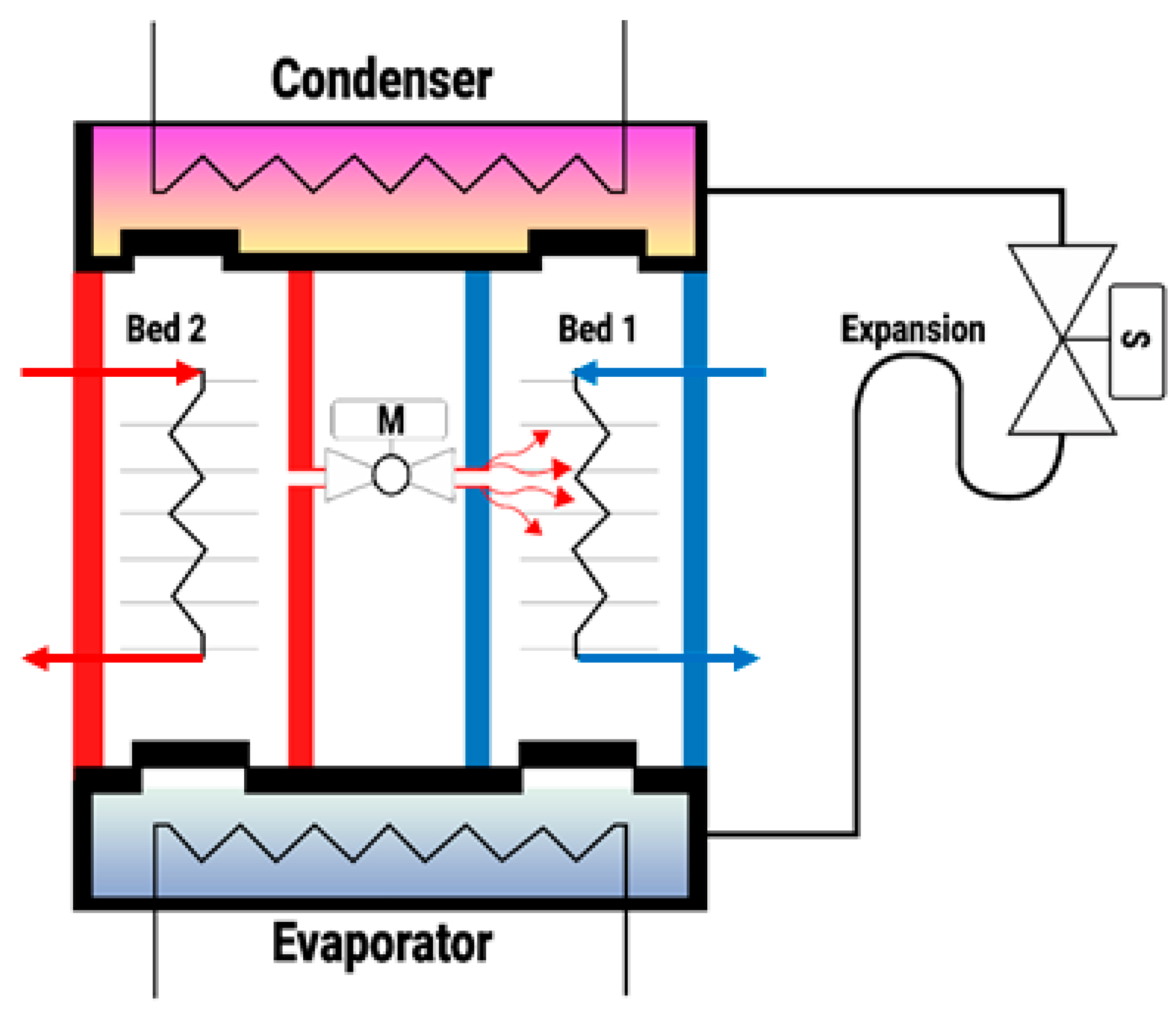
Since the adsorption cooling cycle has a relatively low COP, the mass-recovery concept was developed to improve adsorption cycle efficiency [24]. This concept involves connecting the high-pressure bed (desorber) to the low-pressure bed (adsorber) at the end of the desorption–adsorption cycle, thereby causing the refrigerant in the desorber to be re-adsorbed in the adsorber because of the pressure difference between the two beds, as shown in Figure 1 [25]. Despite the mass recovery process indicating natural movement of the pressurized refrigerant from the desorber to the adsorber without extra heat input, the mass recovery concept is commonly used in the literature even with continuous heat input, which is similar to the reheating cycle concept, as highlighted above.

Figure 1.
Concept of mass recovery.
The effect of mass recovery without the heating process on the adsorption cooling cycle performance at fixed operation temperatures was investigated by Chan et al. [26]. The simulation results showed that mass recovery improved the COP by about 3.9% with a mass recovery time of 4.7 s. Wang [27] developed and tested an adsorption cooling system at various operation conditions, including mass recovery. Incorporating mass recovery resulted in increased cooling capacity and COP (over 10%). Kabir et al. [28] simulated the effect of mass recovery on the performance of a single-stage adsorption cooling system directly driven by solar energy. The study results showed that the mass recovery process improved the overall performance. Ghilen et al. [17] simulated the effect of mass recovery on a silica gel–water adsorption chiller. The mass recovery was found to improve system performance; however, the improvement level was not quantified. The effect of mass recovery on a three-bed adsorption chiller with various heating temperatures was experimentally investigated by Uyun et al. [29]. The results showed that the COP for the cycle with mass recovery was superior to that of the single-stage cycle for heating temperatures below 75 °C. The effect of mass recovery on the adsorption cooling cycle with different hot water temperatures was investigated by Duong et al. [30] with a transient two-dimensional model. The simulation results showed that mass recovery improved the COP up to 5% at 90 °C. The results also showed that the mass recovery had a greater effect at a lower hot water temperature. This conclusion is in agreement with the result of Uyun et al. [29]. The mass recovery effect on a commercial two-bed adsorption chiller was investigated by Muttakin et al. [31] using a transient lumped model. That study investigated the impact of mass and heat recovery on the chiller performance at various hot water, recooling water, and chilled water temperatures, one with 30 °C and two with 28 °C recooling water, with different mass times up to 25 s. The result showed that there were optimum cycle and mass recovery times for maximum efficiency under specified operating conditions.
There are many studies on the adsorption cooling cycle with mass recovery, but there is a shortage of research on adsorption cooling with recooling water, especially at high temperatures, as is done for heating temperature. This study attempted to bridge this gap by investigating the mass recovery effect at various recooling water temperatures up to 50 °C. The main novelty of the study is that it proposes and investigates a variable mode two-bed adsorption chiller working in single stage mode and short, medium, and long mass recovery modes. In practical situations, it is difficult to maintain a constant recooling water temperature, especially using an air-cooled system on a daily or yearly basis. Moreover, this study provides a methodology to determine the optimum recovery in a dynamic way as a ratio of the cooling cycle duration instead of representing it as time in seconds. In addition, the adsorbent pairs used in this study (SAPO-34/water) were analyzed under different isotherm models to find the optimum isotherm model.
2. System Description
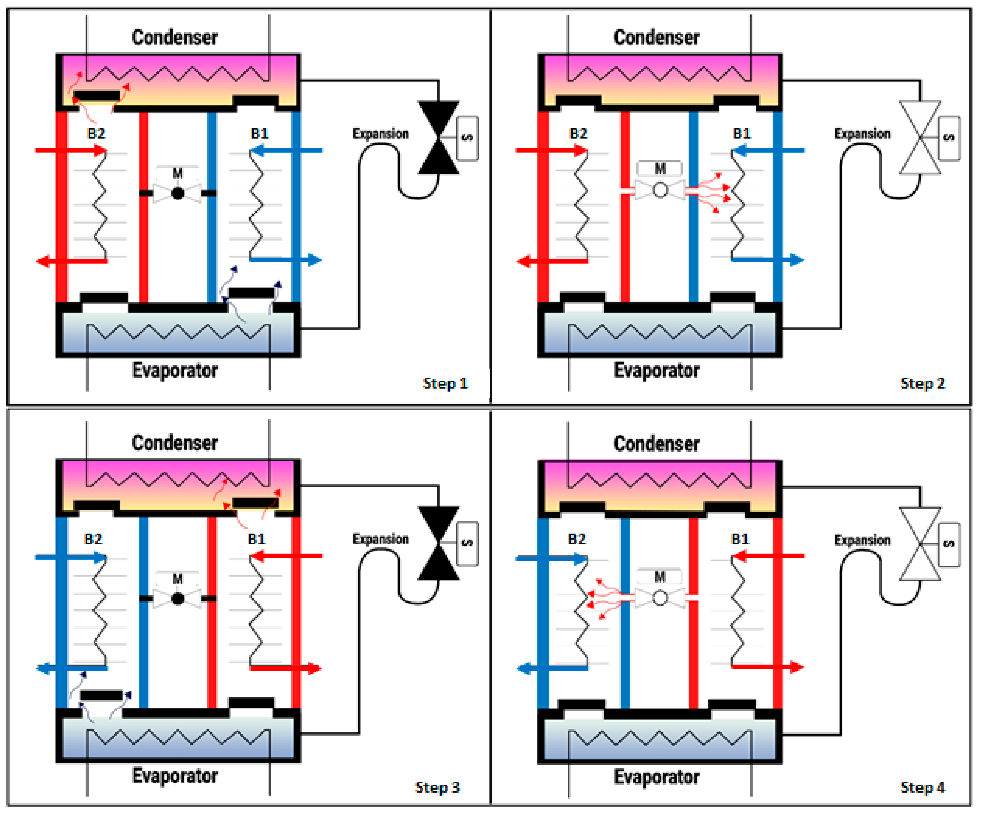
The proposed variable mode adsorption chiller is based on four cycles (steps), as shown in Figure 2. The main concept is to work in a smart way to change the cycle mode based on the ambient or recooling temperature. A patent was filed for this concept by Precision Industries (PI-Dubai) [32]. The working steps can be summarized as follows:
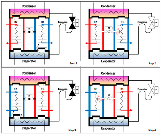
Figure 2.
Variable mode adsorption chiller component.
Step 1: hot water flows into the adsorbent bed (B2), which causes desorption of the refrigerant gases by B2; this increases the pressure inside B2. This forces the gases to flow into the condenser through the non-return valve (NRV). The recooling water flows into the condenser, thereby causing the desorbed hot refrigerant gases to condensate at higher relative pressure and accumulate in the condenser. The condenser is connected to the evaporator with a valve (S) to control the flow based on cycle conditions and the expansion mechanism. The recooling water flows into the adsorbent bed (B1), on which the refrigerant gases are adsorbed, thereby reducing the pressure inside it and forcing the refrigerant to flow from the evaporator to B1 through the NRV. The chilled water flows into the evaporator, thus causing the refrigerant gases to evaporate and travel to B1.
Step 2: the motorized valve (M) opens for a certain time, thus allowing the relative high-pressure hot gases to flow from B2 to B1. The time required for this process depends on the recooling water temperature (mass recovery process with heating and cooling).
Step 3: Valve M closes, and the hot water flows into B1, which causes desorption of the refrigerant gases by B1. This increases the pressure inside B1 and forces the gases to flow into the condenser through the NRV. The recooling water flows into the condenser and the desorbed hot refrigerant gases condensate at a high relative pressure to be accumulate in the condenser. The condenser is connected to the evaporator by a valve (S) to control the refrigerant flow based on the cycle and expansion mechanism. The recooling water flows into B2, causing the refrigerant gases to be adsorbed adsorb, thereby reducing the pressure inside it and forcing the refrigerant to flow from the evaporator to B2 through the NRV. Next, the chilled water flows into the evaporator and causes the refrigerant gases to evaporate and travel to B2.
Step 4: M opens for a certain time, which allows the relative high-pressure hot gases to flow from B1 to B2. The duration of this process depends on the recooling water temperature. Therefore, the optimum time increases at higher ambient temperature (mass recovery process with heating and cooling). Then the cycle returns to step 1 to repeat all steps.
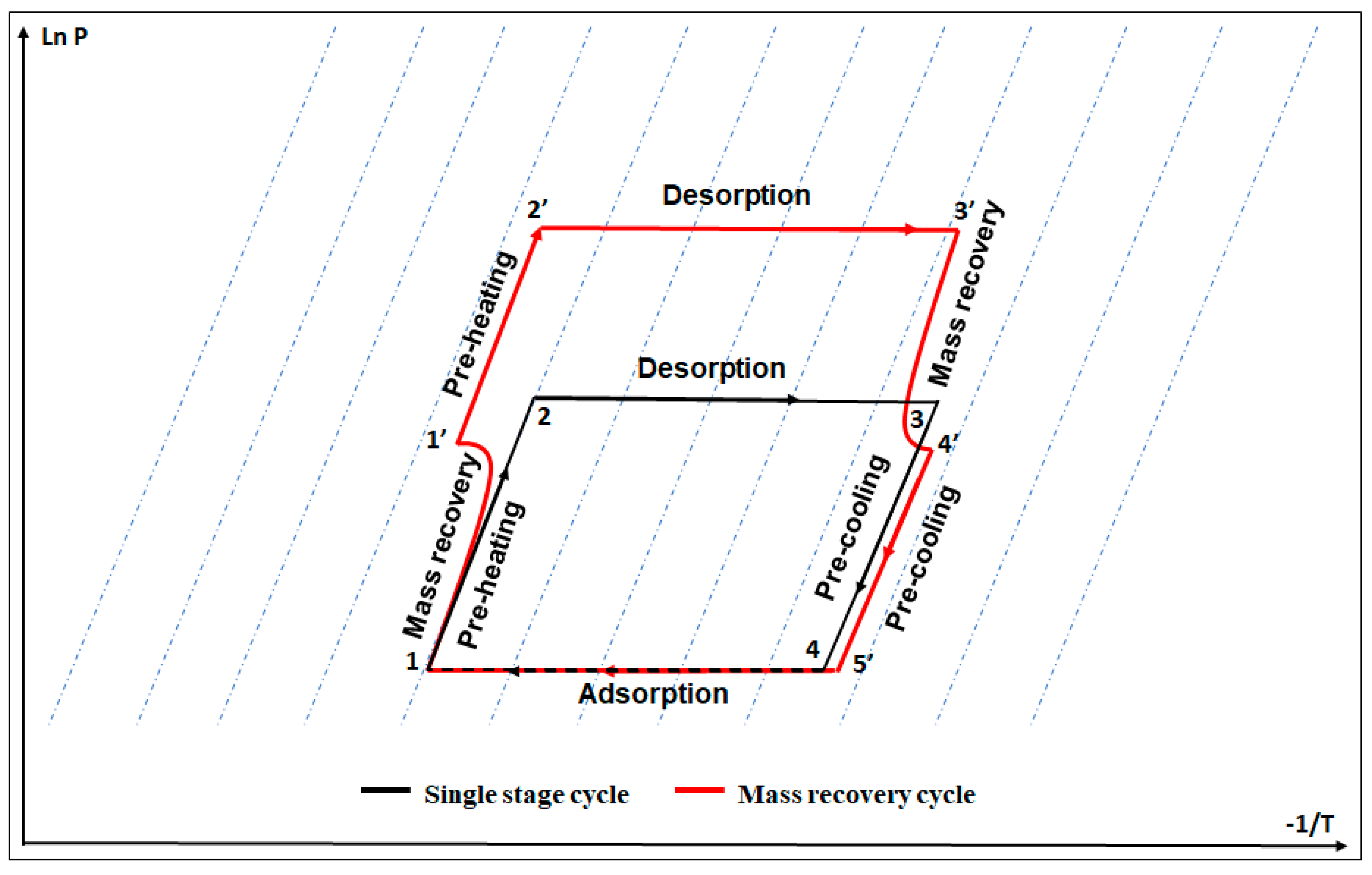
Figure 3 shows a Clapeyron diagram of the thermodynamic processes of the proposed system: the first mode (single stage mode, denoted with 1, 2, 3, and 4) and other modes (mass recovery cycle with heating and cooling, denoted with 1, 1′, 2′, 3′, 4′, and 5′). The cooling capacity in the mass recovery mode (represented as the net area in the closed loop) is larger than that during the basic cycle. In addition, the condenser pressure increases, which leads to condensation at a higher temperature. For the first mode, there are four thermodynamics processes: preheating (1–2), desorption (2–3), precooling (3–4), and adsorption (4–1). In the second mode, there are six thermodynamics processes: mass recovery/adsorption with pressurization when the two beds are connected (1–1′), preheating (1′–2′), main desorption process (2′–3′), mass recovery/desorption with depressurization (3′–4′), precooling (4′–5′), and the main adsorption process (5′–1).
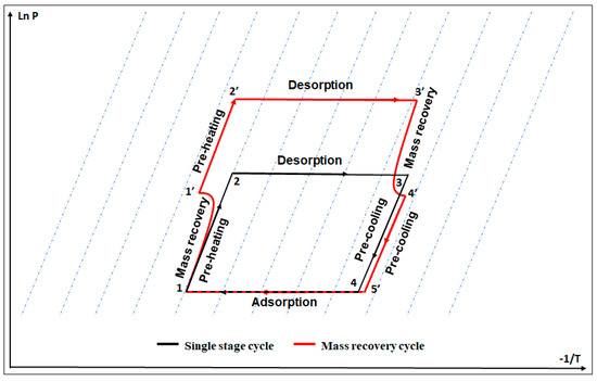
Figure 3.
Clapeyron diagram of variable mode adsorption cooling cycle.
3. Materials and Methods
3.1. Adsorbent Material Characterization
In this study, SAPO-34 zeolite was coated on a heat exchanger using epoxy binder [33], and its properties were investigated with regard to adsorption cooling applications. The microstructure of the zeolite crystals was observed via scanning electron microscopy (SEM) using quanta 250 FEG; the zeolite radius was observed to be approximately 5–10 µm, as shown in Figure 4.
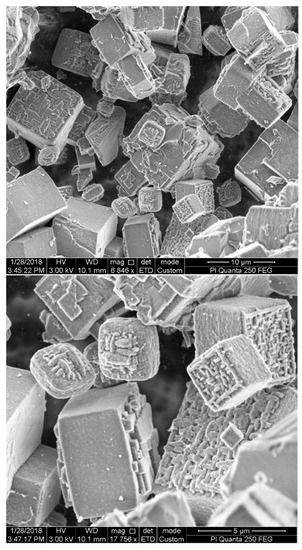
Figure 4.
SEM image of SAPO-34 zeolite.
3.2. Experimental Determination of Adsorption Isotherms and Adsorption Kinetics
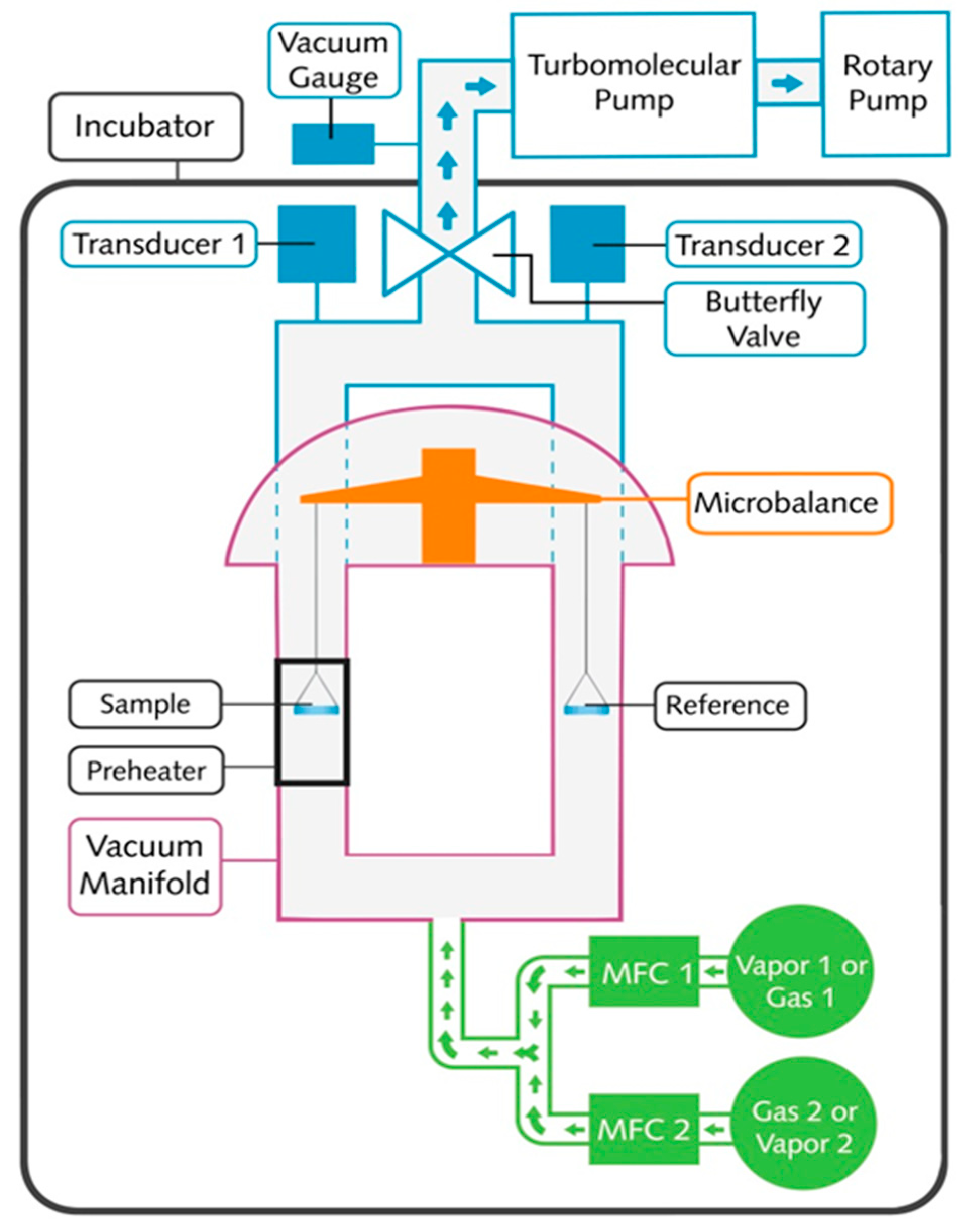
The experimental procedure for determining the adsorption kinetics and isotherms for fitting with various mathematical models are explained in this section. The equilibrium of the water uptake for SAPO-34 was determined using a dynamic vapor sorption (DVS) analyzer (Surface Measurement Systems Ltd., London, UK). A schematic diagram of DVS is shown in Figure 5. Water sorption isotherms of up to 90% P/P0 at temperatures of 20–70 °C were measured using DVS. The data were recorded in the dynamic mode every 20 s, wherein both the sorbate entry rate, controlled upstream by a mass flow controller, and the sorbate exit rate, controlled downstream by a butterfly valve, were measured. Throughout the experiment, the pressure in the vacuum chamber was controlled (from 1.33 to 133.3 kPa) using a butterfly valve (Baratron by MKS Instruments) that regulated the sorbate exit rate depending on the feedback and adjusted the opening position to maintain the set pressure. A mass flow controller was used to maintain a constant flow rate for the water vapor that was generated at an experimental temperature under thermodynamic equilibrium. Variations in the sample mass were simultaneously measured using an UltraBalance (Surface Measurement Systems Ltd., UK). The sample was kept under constant water-vapor pressure until the mass equilibrium was attained, before the water vapor pressure was increased (adsorption branch) or decreased (desorption branch). The water adsorption isotherms were recorded for 0–90% P/P0 and for desorption from 90 to 0% P/P0 at three different temperatures. The samples were outgassed in situ at a temperature of 150 °C under high vacuum (<1.33 × 10⁻³ Pa) and cooled to the desired sorption temperature before each sorption experiment. The water sorption measurements were recorded at 34, 40, and 70 °C.
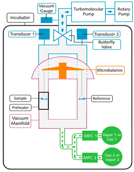
Figure 5.
Schematic of DVS vacuum.
3.2.1. Adsorption Isotherms
The isotherm parameters of SAPO-34/water were calculated using several adsorption isotherm models with details provided in Table 1.

Table 1.
Adsorption isotherm equations for different models.
These models were fitted to the experimental results with the least-squared method using the ‘nlinfit’ function in MATLAB. Root-mean-square error (RMSE) and coefficient of determination (R2) were used to assess the goodness of fit.
3.2.2. Rate of Adsorption
The linear driving force (LDF) model was used to calculate the adsorption rate (kinetic) parameters. The values of pre-exponential constant Dso (m2·s−1), and activation energy Ea (J·mol−1) were calculated by fitting the DVS data to the LDF model:
where the terms are defined as follows:
- : instantaneous water uptake (kg·kg−1);
- maximum water uptake (kg·kg−1);
- R: ideal gas constant (J·mol−1·K−1);
- T: adsorption temperature (K);
- Rp: radius of the adsorbent granules (µm);
- Dso: pre-exponential constant of surface diffusivity (m2·s−1);
- Ea: activation energy of diffusion (J·mol−1).
3.3. Adsorption Cooling System Model
In this study, a two-bed adsorption chiller with single stage and mass recovery modes was modelled with the SAPO-34/water pair and numerically and experimentally simulated based on the adsorption isotherms explained in Section 3.2. The lumped model was used to calculate the mass and energy balances, considering the following assumptions:
- The temperature, pressure, and adsorption rates were assumed uniform in the adsorption beds, evaporator, and condenser.
- The water vapor flow from an adsorption bed to the condenser or from the evaporator to an adsorption bed was unrestricted, and the pressure drop was neglected.
- The chiller was well insulated, and there was no heat exchange with the exterior environment.
- The inlet temperatures for hot, recooling, and chilled water were assumed constant.
The energy flow through the main chiller components is illustrated in Figure 6. The amount of heat and mass transfer at each stage was objectively quantified using the lumped model equations (Equations (2)–(24)), as explained subsequently.
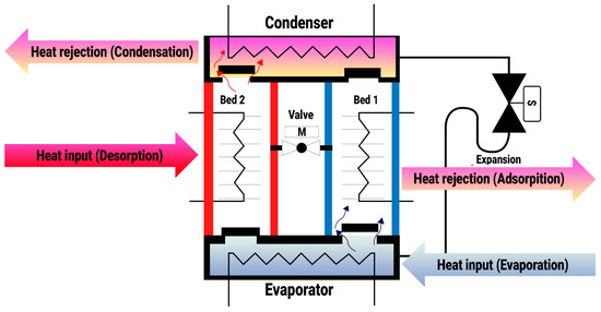
Figure 6.
Schematic of chiller with energy flow.
3.3.1. Energy Balance Equation for the Adsorption Bed
The energy balance equation for the adsorption bed is given as:
where the terms are defined as follows:
- : mass of zeolite in the adsorbent bed (kg);
- : specific heat capacity of zeolite (kJ/kg·K);
- : mass of the adsorbent bed heat exchanger (kg);
- : specific heat capacity of the adsorbent bed heat exchanger (kJ/kg·K);
- : specific heat capacity of water vapor (kJ/kg·K);
- : amount of water in the bed (kg);
- : heat of adsorption (kJ/kg);
- : adsorbent bed temperature (K);
- : water vapor temperature (K);
- : evaporator temperature (K);
- : recooling water mass flow rate (kg·s);
- : recooling water specific heat capacity (kJ/kg·K);
- : recooling water inlet temperature (K);
- : adsorbent bed recooling water outlet temperature (K).
Here, = 1 if the adsorbent bed is connected with the evaporator and 0 if the adsorbent bed is connected with another bed (mass recovery process). The left-hand side of the equation denotes the required sensible heat transfer of the adsorbent bed (SAPO-34, water, and copper heat exchanger). The first part of the right-hand side of the equation shows the adsorbed heat. The second term shows the sensible heat flow from the evaporator to the adsorbent bed. The third term shows the heat transfer by cooling water.
The cooling water outlet temperature is calculated using
where the terms are defined as follows:
- : the overall coefficient of heat-transfer (kW/m2·K) for the adsorbent bed;
- : the area (m2) of the adsorbent bed.
The overall heat transfer coefficient of the adsorbent bed is calculated in this study experimentally based on:
where is the adsorption heat capacity and LMTD is the log mean temperature difference being calculated as:
3.3.2. Energy Balance Equation for the Desorption Bed
The energy balance for the desorption bed is described as:
where the terms are defined as follows:
- : the mass flow rate (kg/s);
- : the specific heat capacity (kJ/kg·K);
- : the inlet temperature (K);
- : the outlet temperature (K).
The left-hand side of the equation shows the required sensible heat transfer for the adsorbent bed (SAPO-34, water, and copper heat exchanger). The first part on the right-hand side of the equation denotes the desorption heat, and the second term indicates the heat transferred by heating water.
The hot water outlet temperature can be calculated by:
where the terms are defined as follows:
- : the overall coefficient of heat-transfer (kW/m2·K) of the desorber;
- : the area (m2) of the desorber.
The overall coefficient of heat-transfer of the desorber is calculated in this study experimentally based on below Equation (14):
where is the desorption heat capacity and LMTD is the log mean temperature difference:
3.3.3. Energy Balance Equation for the Condenser
The energy balance for the condenser is described as:
where the terms are defined as follows:
- : mass of water inside the condenser (kg);
- : mass of the condensing heat exchanger (kg);
- : specific heat capacity of the condensing heat exchanger (kJ/kg·K);
- : latent heat of evaporation (J/kg);
- : recooling water mass flow rate (kg/s);
- : condenser temperature (K);
- : adsorbent bed recooling water outlet temperature (K).
Here, the left-hand side of the equation shows the required sensible heat transfer of the condenser water and the copper heat exchanger. The first part on the right-hand side denotes the latent heat of vaporization for water. The second term indicates the sensible heat transfer from the desorber to the condenser. The third term denotes the heat released by the cooling water.
The cooling water outlet temperature of the condenser water can be calculated by:
where the terms are defined as follows:
- : the condenser temperature (K);
- : the overall coefficient of heat-transfer (kW/m2·K);
- : the condenser area (m2).
The overall coefficient of heat-transfer of the condenser is calculated as:
where is the adsorption and condensation heat capacity, and LMTD is the log mean temperature difference:
3.3.4. Energy Balance Equation for the Evaporator
The energy balance for the evaporator is described as
where the terms are defined as follows:
- : mass of water inside the evaporator (kg);
- : mass of the evaporator heat exchanger (kg);
- : specific heat capacity of the evaporator heat exchanger (kJ/kg·K);
- : evaporator temperature (K).
For the chilled water:
- : mass flowrate (kg/s);
- : specific heat capacity (kJ/kg·K);
- : inlet temperature (K);
- : outlet temperature (K).
The left-hand side of the equation represents the required sensible heat transfer of the evaporator (copper heat exchanger and water). The first part of the right-hand side indicates the latent heat of water vaporization. The second term represents the sensible heat required to cool down the incoming condensed water to the condensation temperature. The third term represents the heat transfer by the chilled water.
The chilled water outlet temperature was calculated using:
where the terms are defined as follows:
- : the overall coefficient of heat-transfer (kW/m2·K);
- : the area of the evaporator (m2).
The overall coefficient of heat-transfer of the evaporator is calculated in this study based on:
where is the adsorption and evaporation heat capacity and LMTD is the log mean temperature difference:
3.3.5. Mass Balance
The system mass balance is described by:
where the terms are defined as follows:
- : the mass of water (refrigerant) entering the evaporator (kg);
- : the mass of zeolite in the bed (kg).
3.3.6. System Performance
The cooling capacity Q and the COP of the system were calculated using Equations (28) and (29), respectively. The COP represents the ratio of cooling capacity to the required heat input; the COP of the system is calculated based on the total cycle period (tcy), including periods for precooling, adsorption, preheating, and desorption.
The proposed model of energy, mass balance, and performance equations were solved numerically by MATLAB using ODE 45 to calculate the temperatures of the adsorption and desorption beds, condenser and evaporator, as well as system performance.
3.4. Experimental Setup
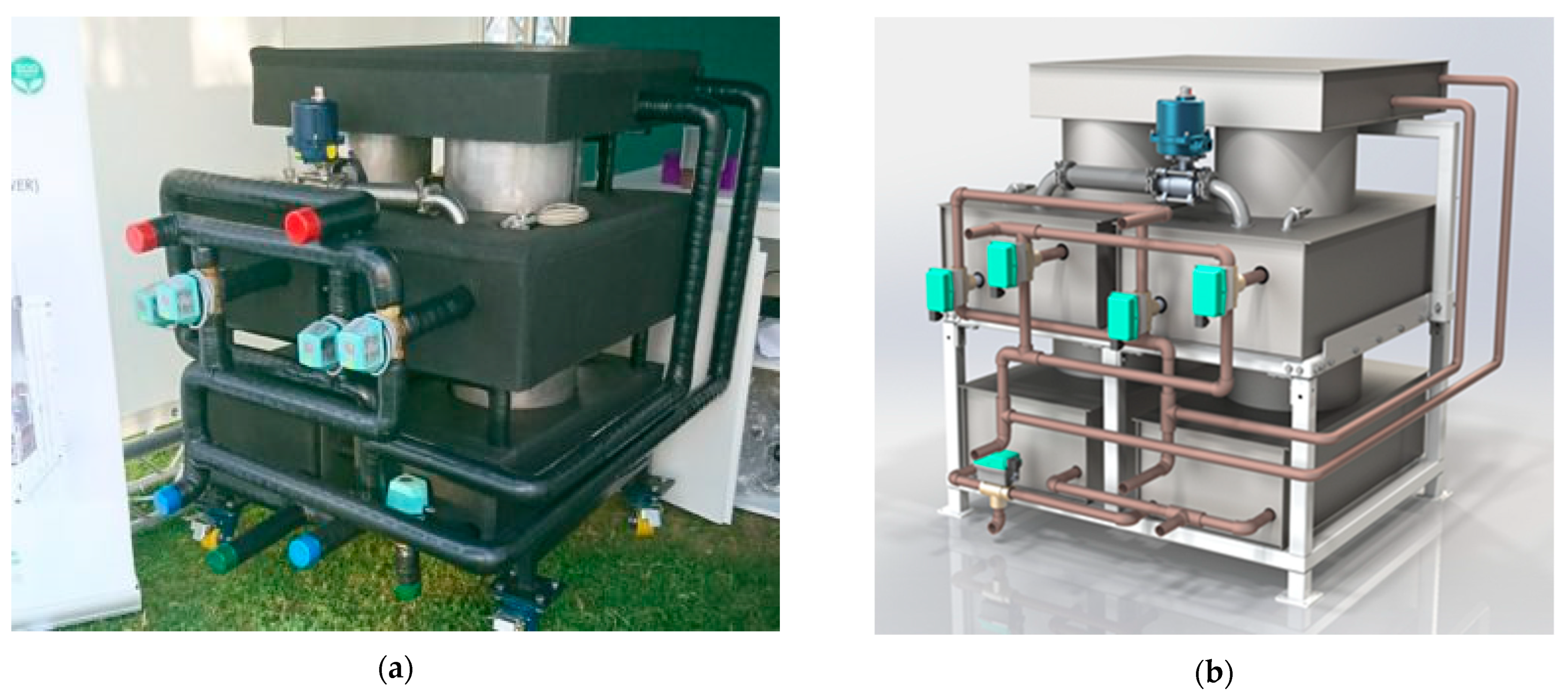
A lab-scale model of the variable cycle chiller was built at the Precision Industries (PI, Dubai) labs to measure the performance of the chiller experimentally under different modes and various recooling temperatures. The proposed tested adsorption chiller in this study consisted of two adsorbent beds coated with SAPO-34 supplied by Mitsubishi Chemical Corporation (see Figure 7).

Figure 7.
PI prototype adsorption chiller: (a) prototype, (b) 3D model.
The chiller performance was analyzed under the following operation conditions:
- The inlet hot water temperature (Th_in) of 90 0.5 °C maintained by an electric water heater with a 500 L buffer tank.
- The inlet recooling water temperature (Tre_in) of 30–50 °C maintained by a dry-cooler with a 500 L buffer tank.
- The inlet chilled water temperature (Tch_in) of 18 0.5 °C maintained by an electrical heater with a 500 L buffer tank, the electrical heater is used as a cooling load in this case.
- Hot, recooling, and chilled water flow rates for were 1.2, 1.2, and 0.71 L/s, respectively.
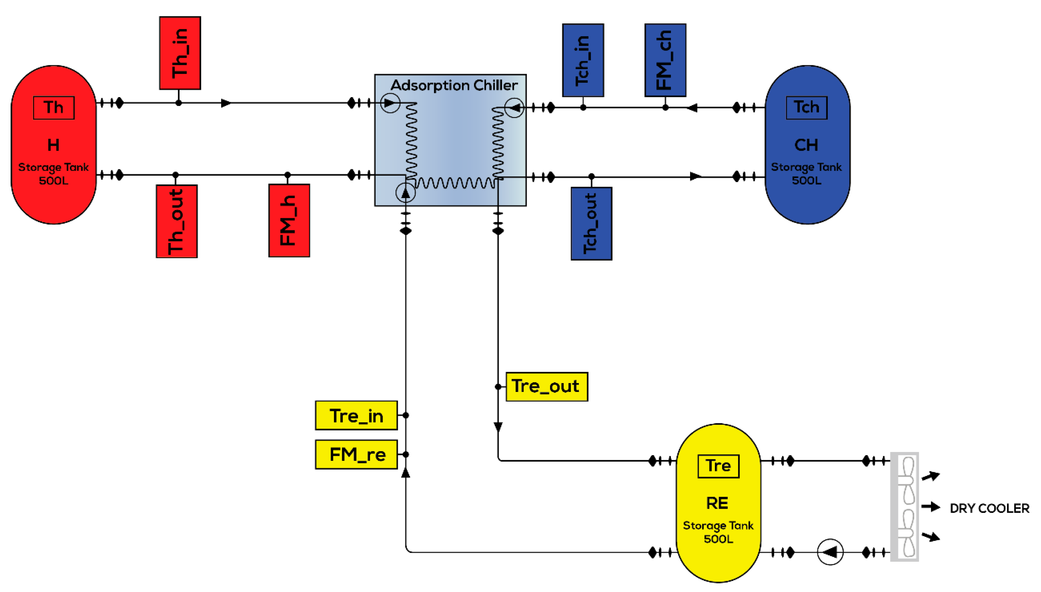
The following setup of instrumentation was used to measure the experimental performance of the chiller during the mass recovery cycle, as shown in Figure 8. The instrument locations are described as follows:
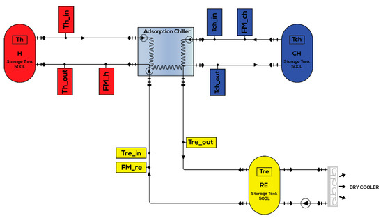
Figure 8.
Schematic of prototype adsorption chiller testing equipment.
- Three electromagnetic flow-meters (FM_h, FM_ch, and FM_re) (manufactured by ALIA Inc., Newark, DE, USA) with accuracy of ±0.4% were used to measure the hot water, chilled water and recooling water flow rate, respectively.
- Eight platinum resistance thermometers (PT100 Class A, Pico Technology) integrated with two temperature measuring data loggers (PT-104 is a four-channel logger), a resolution of 0.001 °C, and an accuracy of 0.015 °C were used to measure the inlet and outlet temperatures of the hot, chilled, and recooling water, as well as temperature of the storage tanks.
4. Results and Discussion
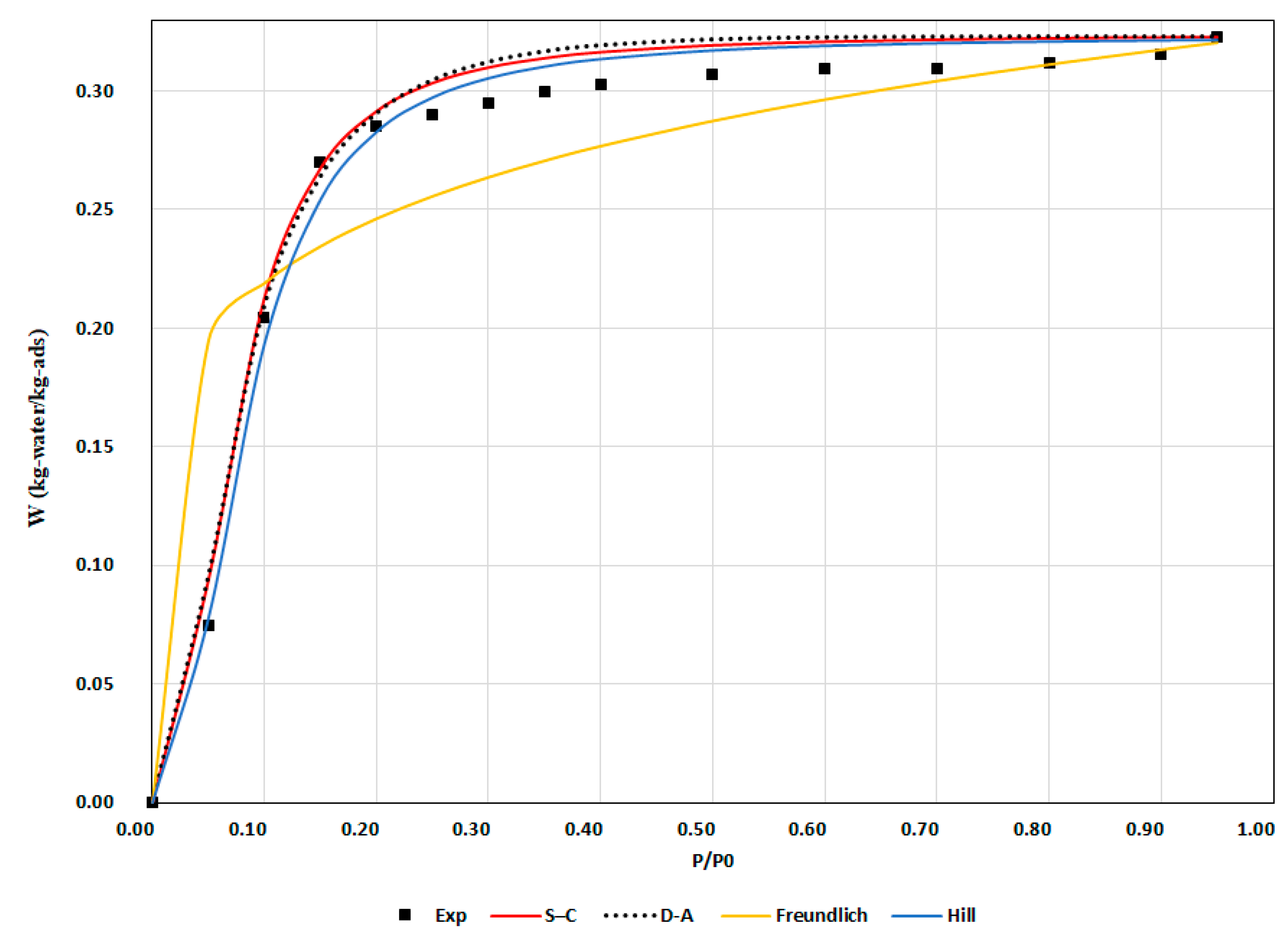
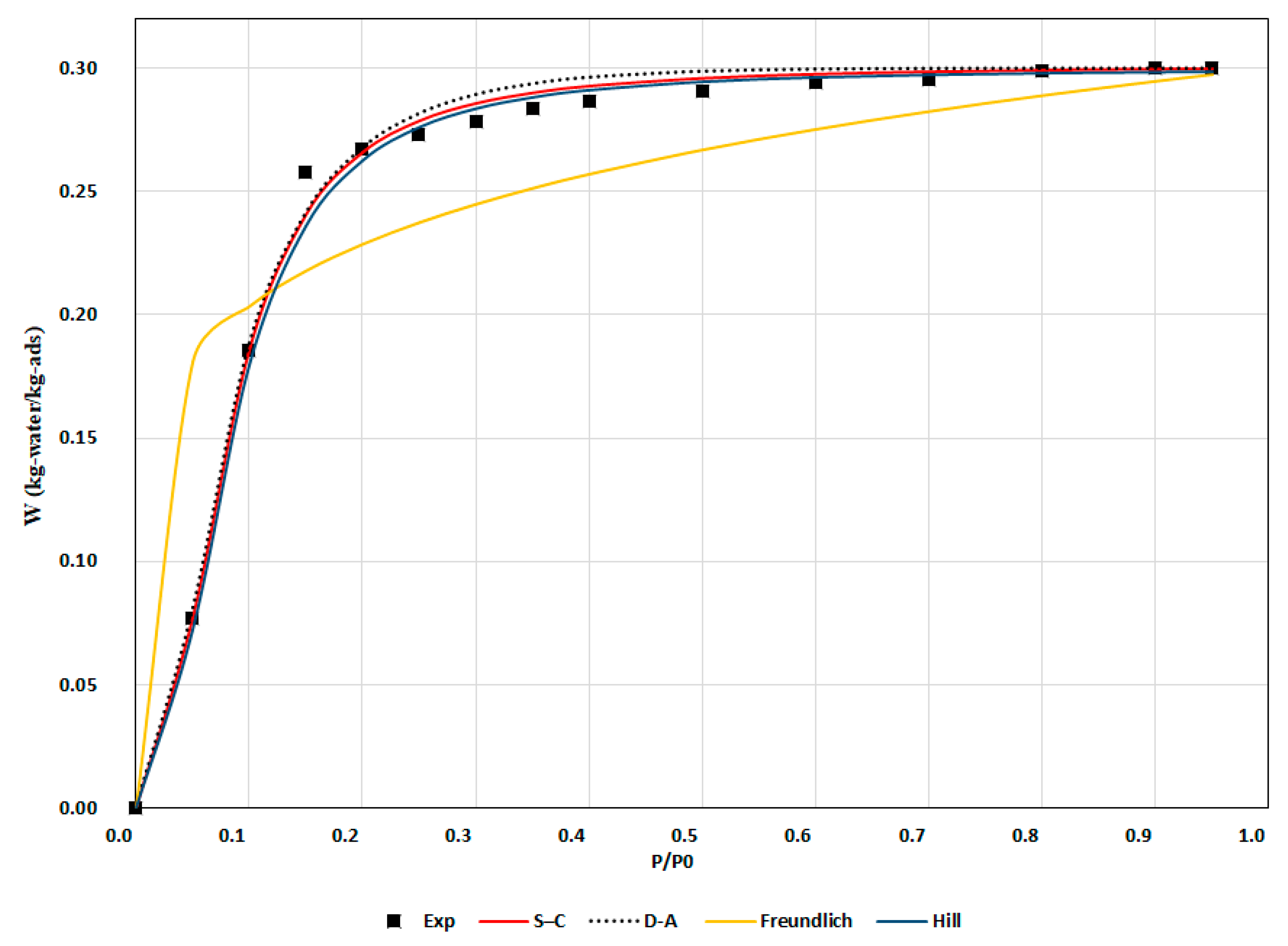
Figure 9, Figure 10 and Figure 11 present the experimental results of water-vapor uptake compared with the calculated values at 34, 40, and 70 °C, respectively. The isotherm parameters for each model are listed in Table 2. As shown in Figure 6, Figure 7 and Figure 8, the D–A, Hill, and S–C models correlated well with the experimental data, whereas the Freundlich model failed to fit.
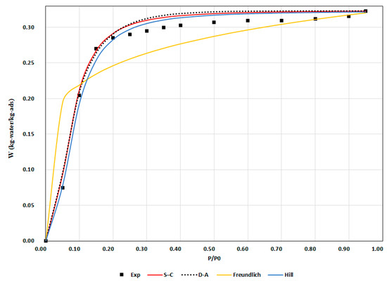
Figure 9.
Water uptake comparison between experimental and isotherm model results at 34 °C.
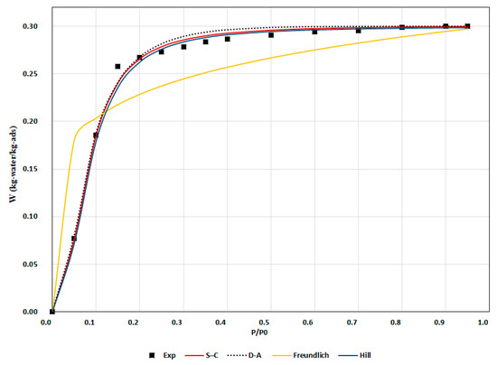
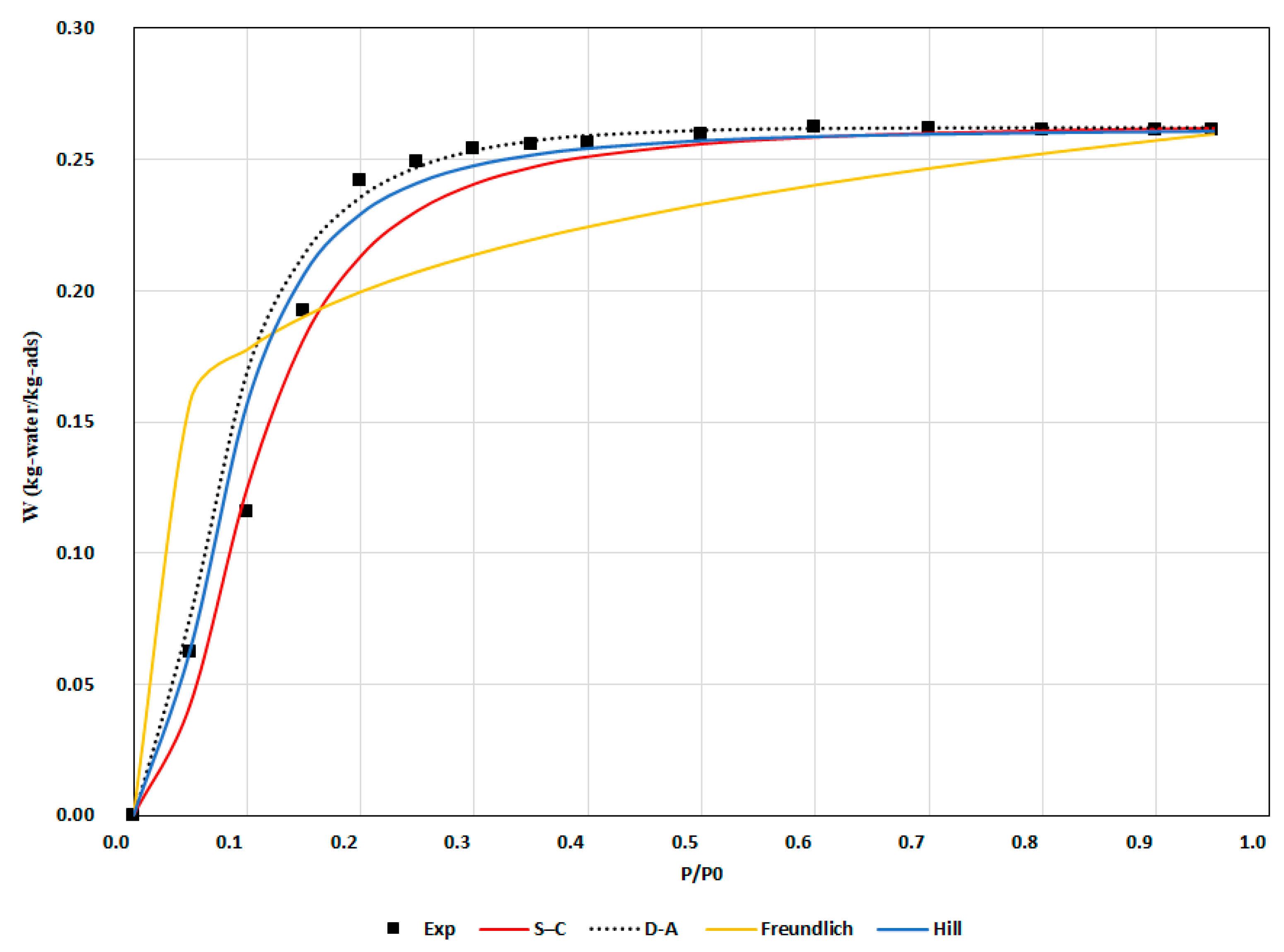
Figure 10.
Water uptake comparison between experimental and isotherm model results at 40 °C.

Figure 11.
Water uptake comparison between experimental and isotherm model results at 70 °C.
Table 2.
SAPO-34 isotherm parameters for different models.
As per the error analysis presented in Table 3, the Hill model exhibited the greatest fitting accuracy at 34 °C, followed by the D–A, S–C, and Freundlich models. At 40 °C, the Hill model achieved the highest fitting accuracy, followed by the S–C, D–A and Freundlich models. The D–A model exhibited the greatest fitting accuracy at 70 °C, followed by the S–C, Hill, and Freundlich models. Overall, the results of the Freundlich model deviated substantially from the experimental results.
Table 3.
Errors and statistical analysis of isotherm fitting results.
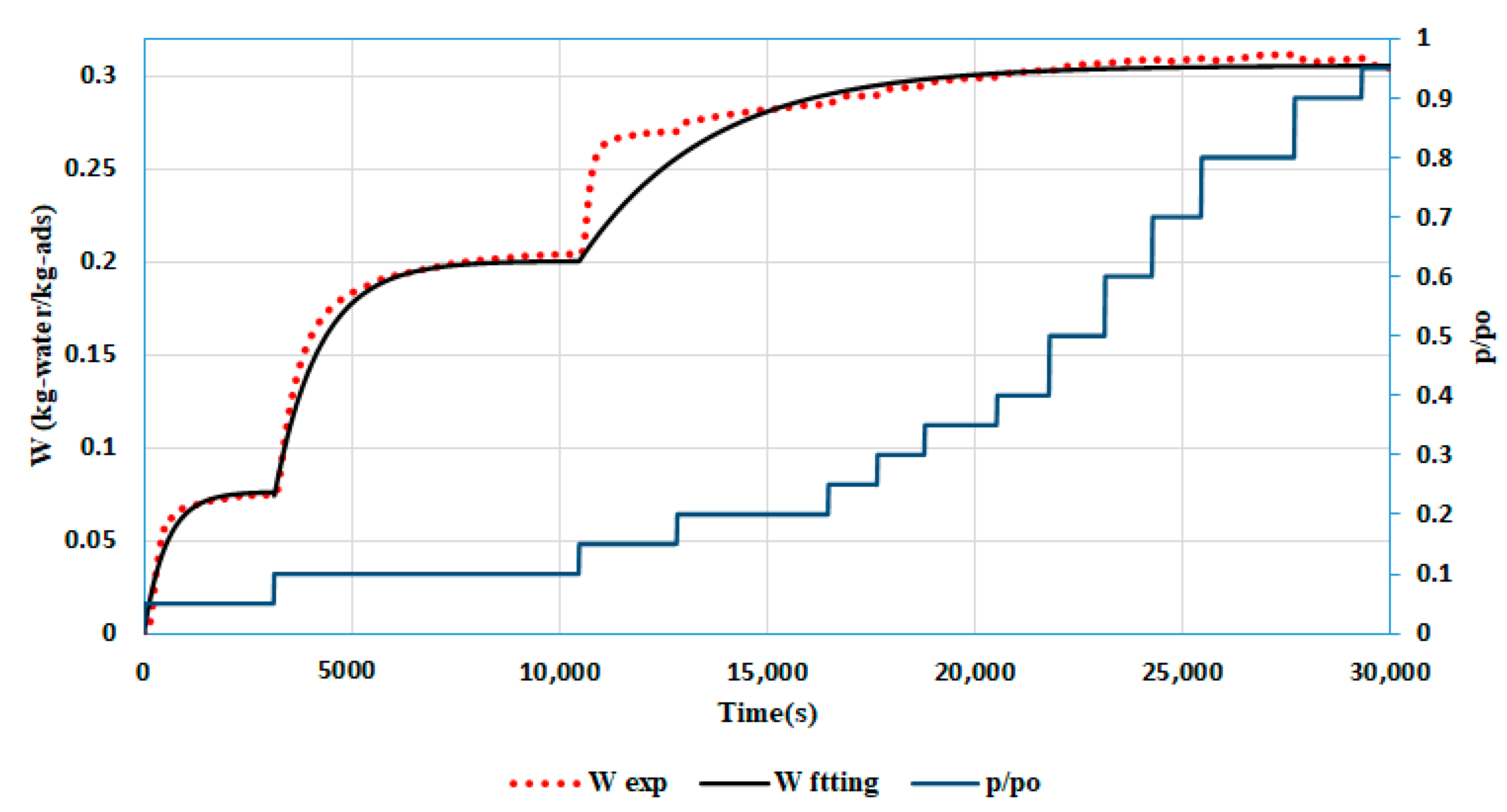
The experimental results of the adsorption kinetics included more than one curve based on the pressure ratios, as shown in Figure 12. The LDF model was fitted to the experimental results for three pressure ratio intervals: P/P0 < 5%, 5% < P/P0 < 15%, and P/P0 > 15%. The fitting results showed that the constants of the adsorption kinetics varied with the partial-pressure intervals; these results are summarized in Table 4. The LDF model was fitted satisfactorily to the experimental data, with an RMSE of 0.0046–0.0119, as shown in Table 4.
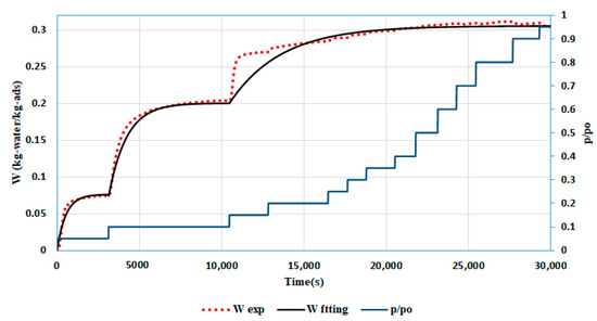
Figure 12.
Adsorption kinetics experiment and fitted results at 34 °C.
Table 4.
SAPO-34 adsorption kinetic parameters with errors and statistical analysis.
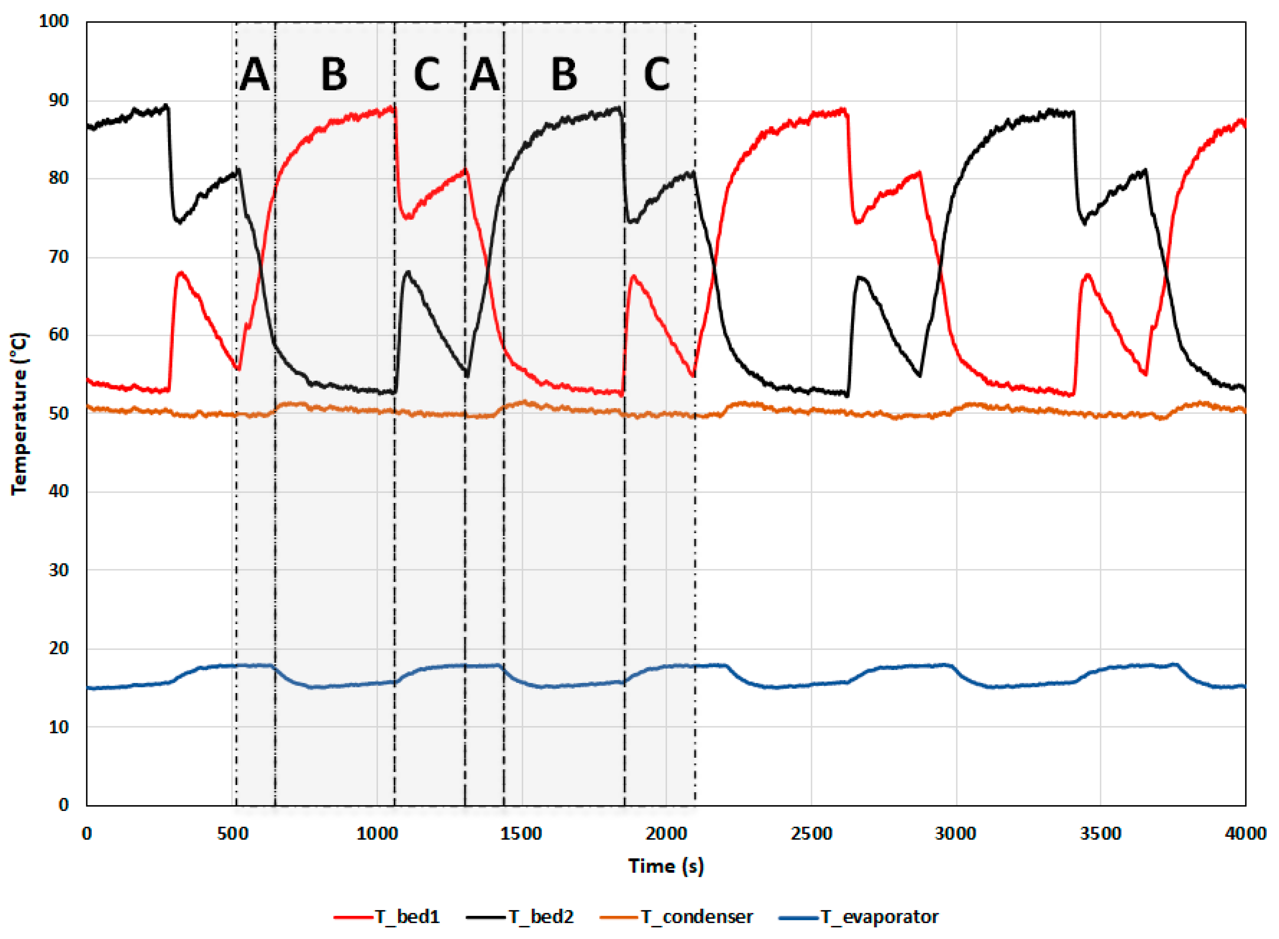
Figure 13 shows the chiller experimental temperature profile at a total cycle time of 750 s and a mass recovery time of 150 s. Areas A, B, and C indicate the preheating/pre-cooling, adsorption/desorption, and mass recovery with heating and cooling processes, respectively, where both beds were connected with no cooling effect.
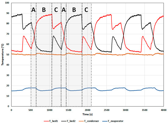
Figure 13.
Experimental temperature profile for prototype adsorption chiller with mass recovery with overall cycle time of 750 s. Thw_in = 90 °C, Tcw_in = 50 °C, and Tchw_in = 18 °C.
Figure 13 shows a cycle period range of 500–1280 s during the preheating of desorption bed 1 (area A). During this process, the temperature increased until it reached a suitable level for desorption, and the pressure increased until the condensation pressure was reached. The condenser exhibited the minimum temperature in this cycle (close to the re-cooling water inlet temperature), and no condensation occurred. Once bed 1 reached a suitable temperature (as shown in area B), the condenser temperature increased, indicating the flow of hot vapor from bed 1 (at condensation pressure or higher) to the condenser. In the pre-cooling phase, the bed 2 temperature decreased until it reached a suitable level for adsorption, and the pressure decreased to less than the evaporator pressure. During this phase, the evaporator exhibited its maximum temperature (close to the chilled water inlet temperature) and no cooling effect occurred. Once bed 2 reached a suitable temperature and pressure for adsorption, the evaporator temperature decreased and the cooling effect occurred (area B). In the mass recovery process (area C), there was a sudden drop in temperature in bed 1 (desorber) and an increase in bed 2 (adsorber). This can be attributed to the increase in adsorption and desorption rates immediately after interconnecting both beds until equilibrium pressure was reached. The desorber temperature then started to increase and the adsorber temperature started to decrease owing to the decrease in adsorption and desorption rates occurring later in the process. Therefore, the heat input became higher than the amount required for desorption, and the rejected heat increased to values higher than the heat of adsorption.
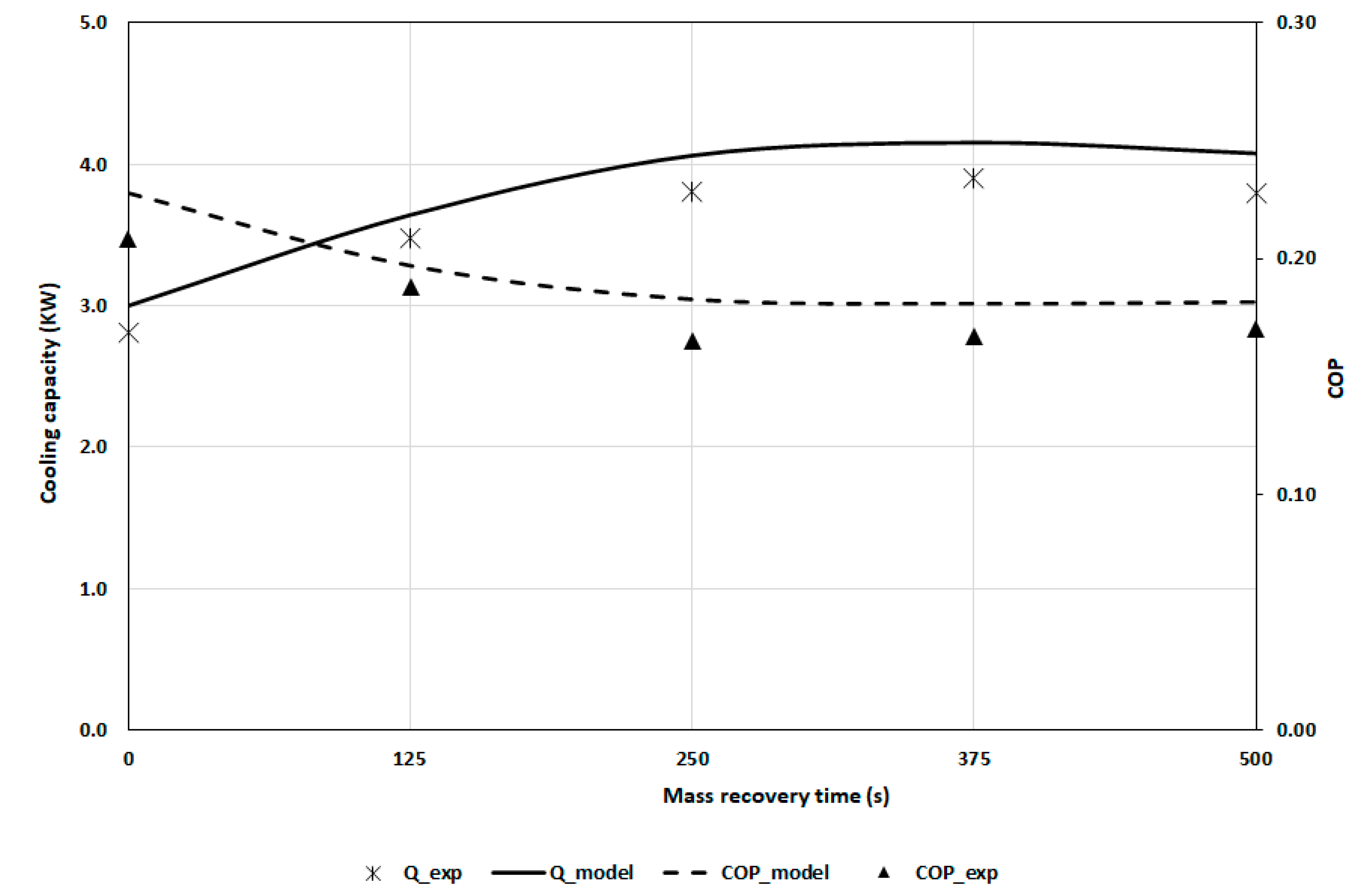
The system was investigated at a cooling cycle time of 500 s with different mass recovery times. Figure 14 shows a comparison between the COP and cooling capacity for the simulated model and the experimental measurements, which matched the predicted results and showed the same trends. The mean absolute percent errors for COP and cooling capacity were 9.5% and 6.8%, respectively. Figure 14 indicates that as the mass recovery process time increased, the COP decreased until a saturation trend was observed, where the COP remained constant. In addition, as the mass recovery time increased, the cooling capacity increased until a saturation trend was observed, where the cooling capacity was not affected by the mass recovery process time. In both cases, for COP and cooling capacity, the curve drops for high cycle times.
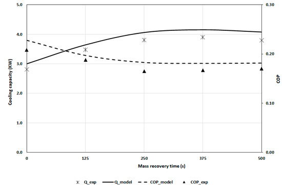
Figure 14.
Comparison between experimental and predicted COP and cooling capacity with various mass recovery times at Thw_in of 90 °C, Tcw_in of 50 °C, and Tchw_in of 18 °C.
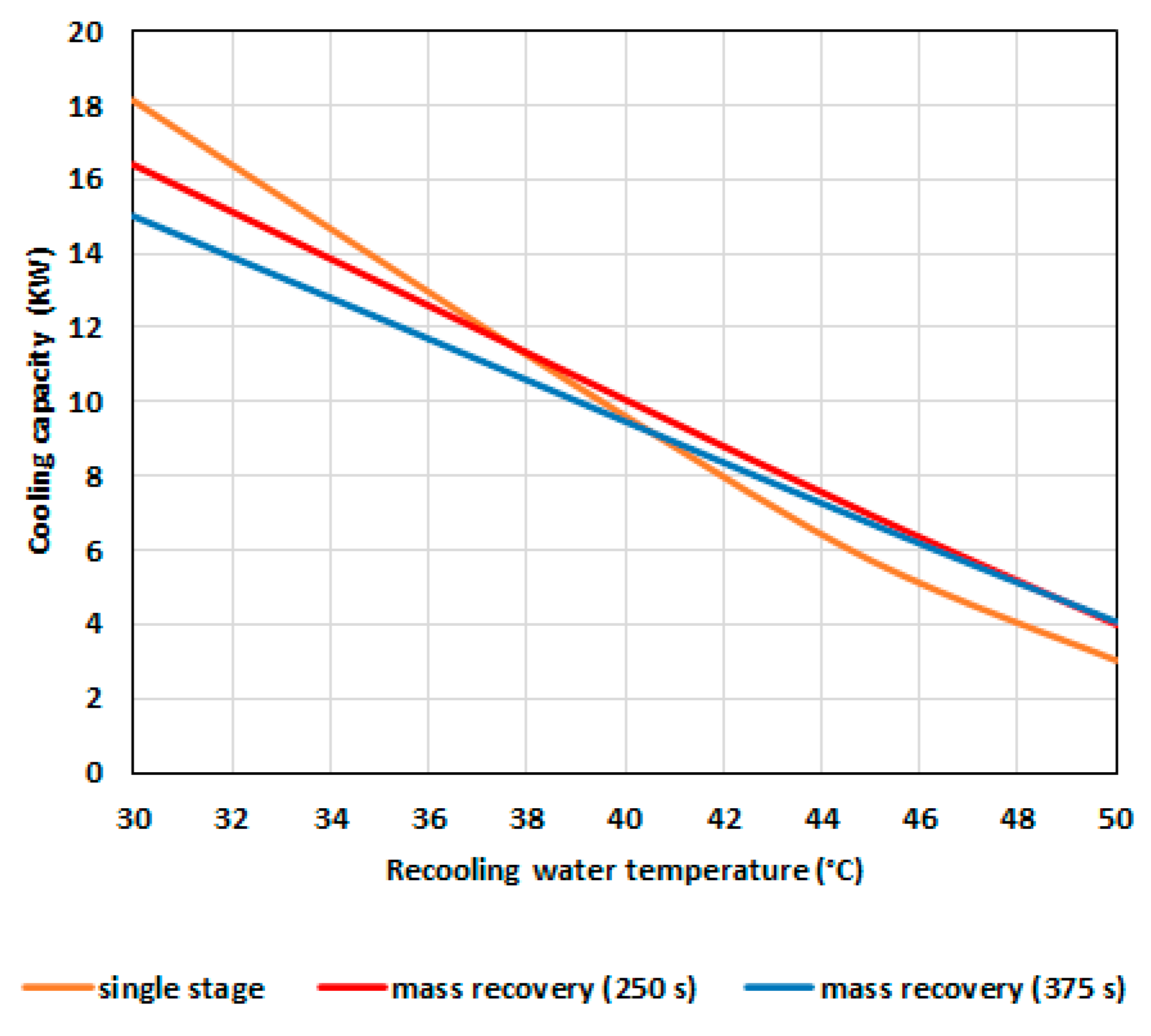
Figure 15 shows the simulation results of cycle cooling output at different recooling water temperatures, with single stage cycle and two mass recovery durations at a fixed cooling cycle duration of 500 s. The single stage cycle exhibited better cooling output at a recooling temperature below 38 °C compared to higher recooling water temperature. The mass recovery cycle of 250 s exhibited higher cooling output within a recooling water temperature range of 38–49 °C, while the mass recovery cycle of 375 s exhibited a higher output at a recooling water temperature higher than 49 °C.
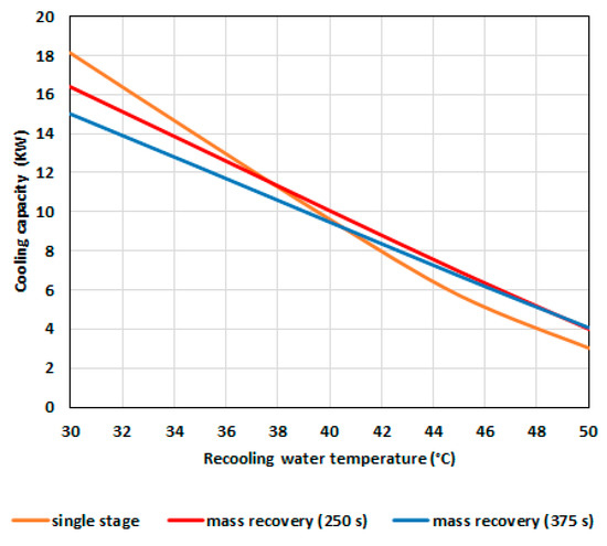
Figure 15.
Predicted cooling capacity with various mass recovery times and recooling water temperatures.
The simulated COP results are shown in Figure 16. For a fixed cycle time of 500 s, the simulation shows that the single stage cycle shows the highest COP at various recooling water temperatures. In addition, the COP of the 250 s mass recovery cycle was higher than that of the 375 s mass recovery cycle up to a recooling water temperature of 50 °C, whereas at higher temperatures, similar COP values were seen. These results prove the importance of the variable-cycle mode adsorption cooling system to optimize the chiller performance with changes in recooling temperature.
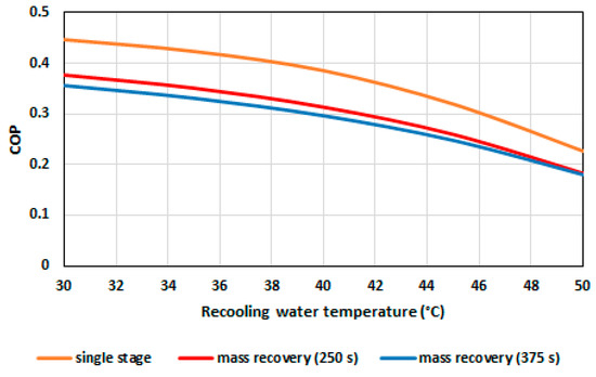
Figure 16.
Predicted COP with various cycle stages and recooling water temperatures.
The cycle time has a significant effect on cooling capacity and COP. Therefore, the variable mode cycle was simulated using the model at different cycle times and with various recooling water temperatures to further understand their effects. The mass recovery duration is defined in terms of the ratio of cooling cycle duration, reflecting its dynamic value in a comparable manner. The following four modes were investigated in this study:
- First mode: single stage.
- Second mode: mass recovery with heating and cooling; the duration was 25% of the cooling cycle duration (denoted as short mass recovery mode).
- Third mode: mass recovery with heating and cooling; the duration was 50% of the cooling cycle duration (denoted as medium mass recovery mode).
- Fourth mode: mass recovery with heating and cooling; the duration was 75% of the cooling cycle duration (denoted as long mass recovery mode).
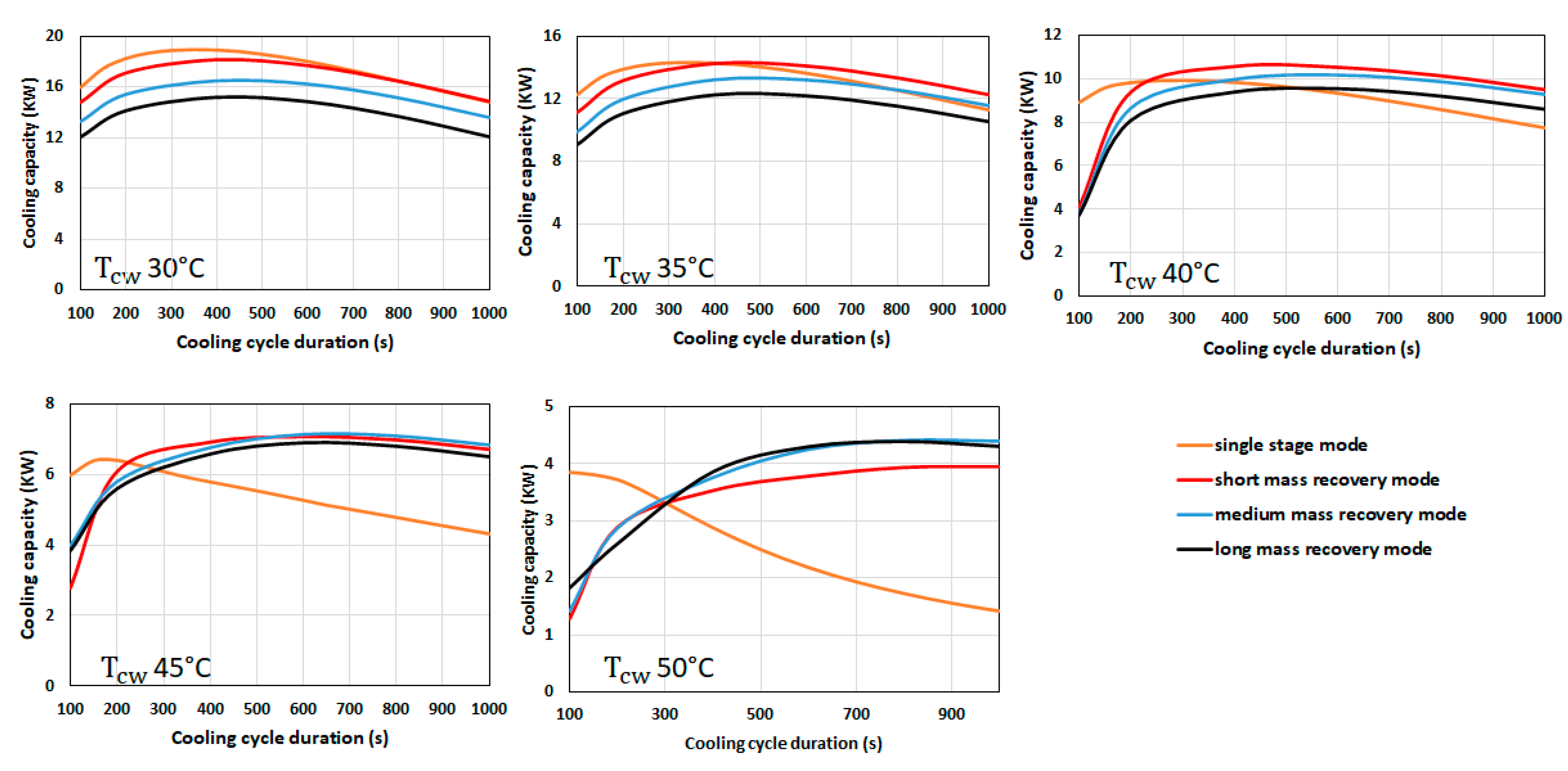
Figure 17 illustrates the modelling results at fixed inlet hot and chilled water temperatures of 90 and 18 °C, respectively. At a low recooling water temperature of 30 °C and a cycle time up to 600 s, the single stage mode exhibited higher capacity than the other modes (see Figure 17). However, at a longer cycle time (more than 600 s), the short mass recovery mode exhibited similar single-stage cooling capacity. With increased recooling water temperature, the system required longer mass recovery time to achieve higher (peak) capacity. Therefore, the uptake of the adsorber should be increased and that of the desorber should be decreased. This can be achieved by increasing the pressure in the condenser and the recooling water temperature or decreasing the adsorption pressure.
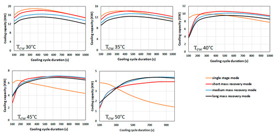
Figure 17.
Predicted cooling capacity at various cycle modes and recooling water temperatures.
There is an optimum mode for each recooling water temperature, which is related to the optimum water vapor uptake and the condensation pressure. Figure 17 shows that cooling capacity increased with increased cooling cycle time until a peak point, after which it decreased. The peak cooling capacity was obtained when sufficient time was allowed to reach the optimum water uptake. With a shorter time, the water vapor uptake and cooling capacity were low because the adsorbent bed failed to reach the minimum temperature and pressure to achieve higher adsorption rates. With a longer time, the uptake of the adsorbent bed increased, thereby leading to a lower adsorption rate and cooling capacity. At a fixed recooling temperature, the cooling capacity decreased with an increase in relative mass recovery time because the cooling time became lower than the total cycle time.
Figure 18 illustrates the COP behavior at low and high recooling water temperatures. It can be seen that the COP increased as the cycle time increased because the cooling effect increased more than the heat input during the pre-heating phase. At a low recooling water temperature, the single stage cycle had a higher relative COP compared to the mass recovery cycle at a cooling cycle time less than 900 s and at a longer cycle time the short mass recovery had a higher COP. At a higher recooling water temperature of 50 °C the single stage cycle had a higher cooling cycle time of less than 750 s. While the mass recovery cycle had a higher COP at longer cooling cycle time, the long mass recovery duration had a higher COP followed by medium and short mass recovery duration.
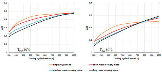
Figure 18.
Predicted COP at various cycle mode and recooling water temperatures.
During adsorption cooling, when the heat source is unlimited to waste heat or another free heat source, the cooling capacity value is higher than the COP. Therefore, in this study, the optimum mode cycle time was selected based on the maximum system cooling capacity. Table 5 shows the optimum cooling cycle time (OCCT) for each mode at various recooling water temperatures.
Table 5.
Optimum cycle time for each cycle mode.
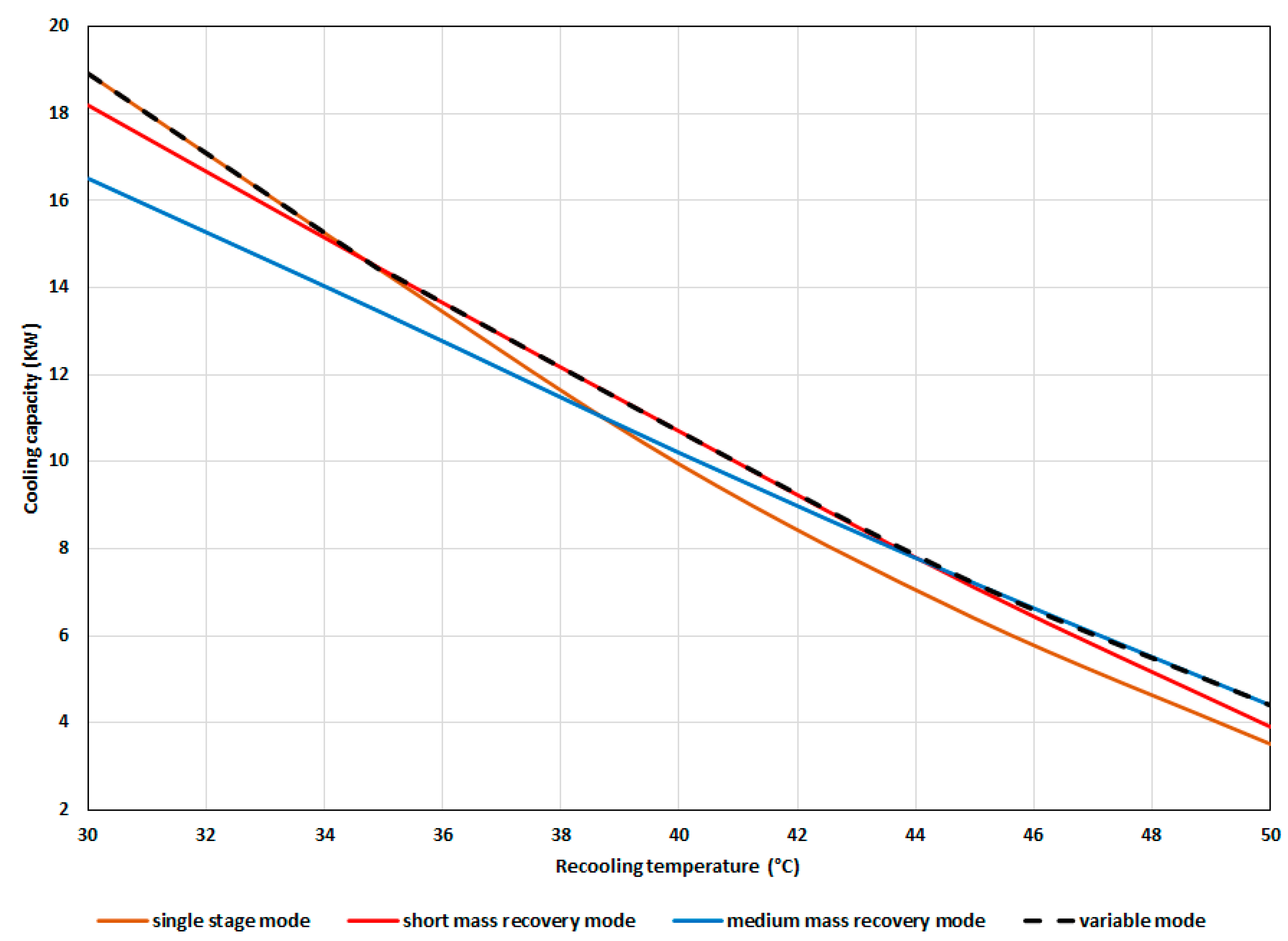
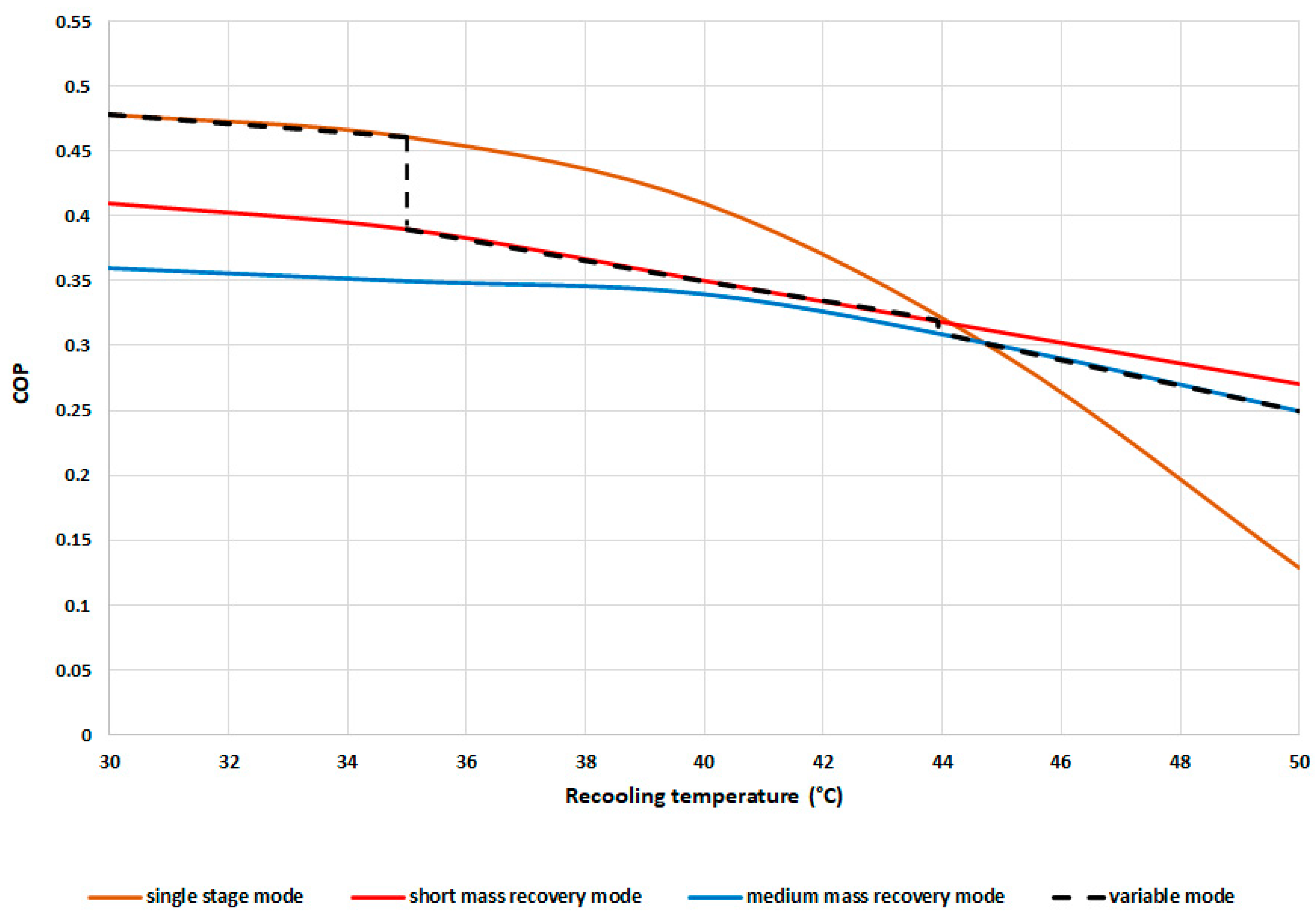
Figure 19 shows the cooling capacity at optimum cycle time for the different modes with different recooling water temperatures. The variable mode curve follows the optimum cooling capacity at different recooling water temperatures. At recooling water temperatures of 30–35, 35–44, and >44 °C, the single stage cycle, short mass recovery mode, and medium mass recovery mode, respectively, are found to be optimum modes.

Figure 19.
Predicted cooling capacity for various modes and recooling water temperatures.
Under the same conditions listed in Table 5 and Figure 19, the COP at the optimum cycle time for the single stage, short mass recovery, medium mass recovery, and variable modes at various recooling water temperatures is shown in Figure 20. As explained previously, the variable mode tracks the optimum mode based on the cooling capacity. At recooling water temperatures of 35–44 °C, the variable mode COP drops to match that of the short mass recovery mode. At recooling water temperatures of 44–50 °C, the COP drops to match the medium mass recovery cycle mode.
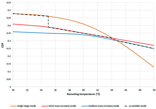
Figure 20.
Predicted COP for various modes and recooling water temperatures.
This result suggests that the working ambient and recooling water temperatures are very important factors affecting COP cycle optimization. At an ambient temperature where the recooling water temperature is less than 35 °C, the single stage mode is recommended to obtain a higher COP; at higher temperatures, the short mass recovery mode is recommended. If the system changes between the two temperature ranges, a variable mode cycle is recommended.
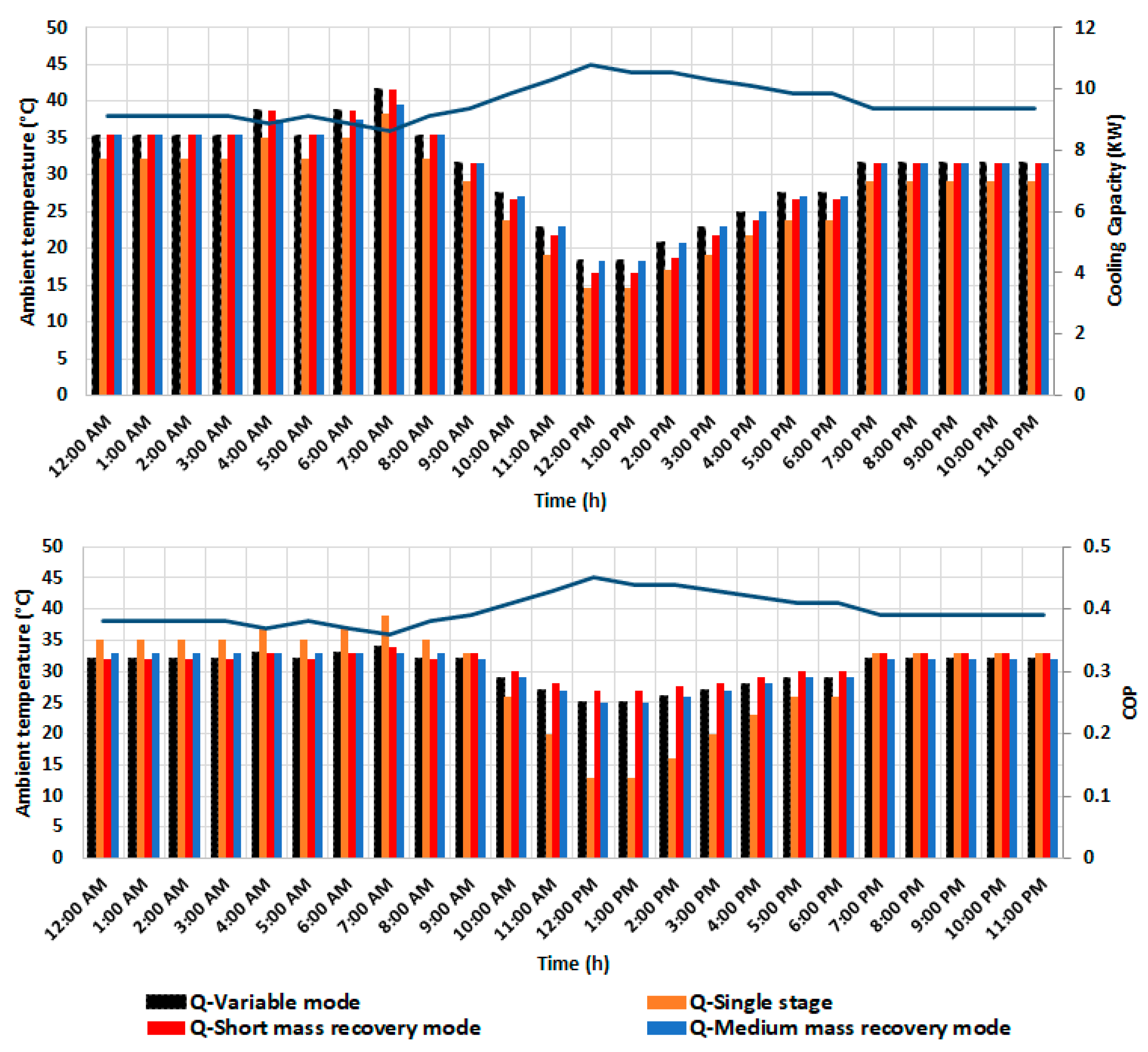
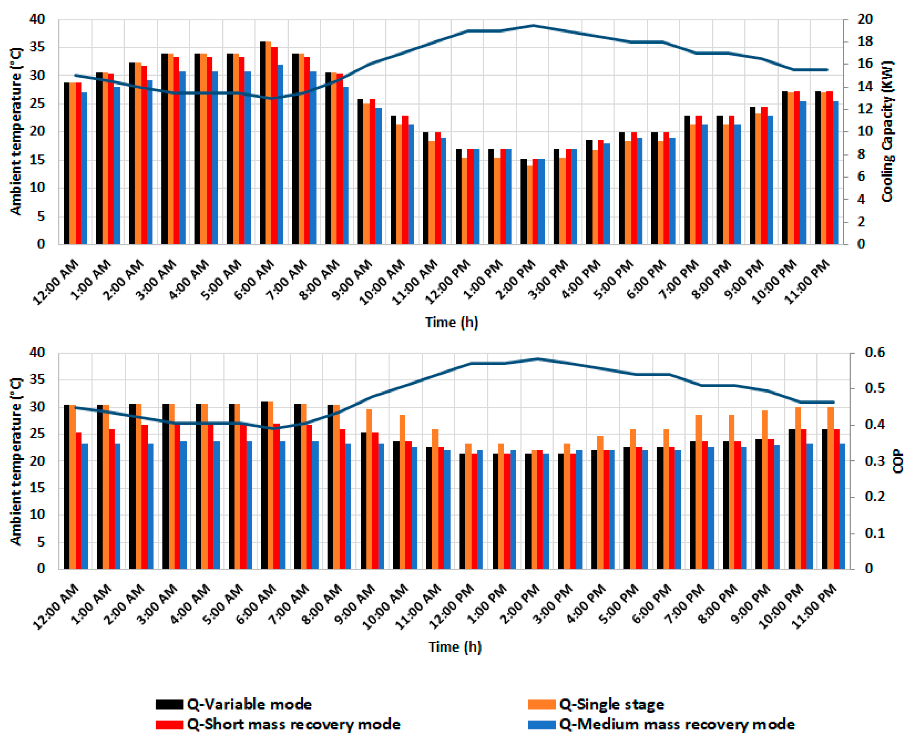
To quantify and assess the air-cooled variable mode adsorption cycle, it is important to reflect on the ambient temperature profile. Figure 21 and Figure 22 show hourly ambient temperature profiles for two days in Dubai. The figures show hourly simulation of the cooling output and COP for different modes based on the predicted chiller performance curves, assuming the temperature changes on an hourly basis and the recooling water temperature is 5 °C higher than the ambient temperature. On day 1, the variable model gives higher daily cooling capacity and COP of 12% and 3.6% compared to the single stage mode. On day 2, the variable mode gives 3.3% higher cooling capacity and 7.7% lower COP compared to the single stage mode.
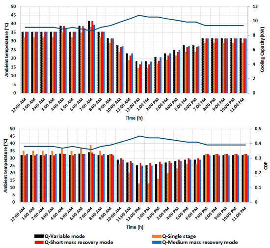
Figure 21.
Measured ambient temperature and expected cooling capacity and COP for various modes (day 1).

Figure 22.
Measured ambient temperature and expected cooling capacity and COP for various modes (day 2).
5. Conclusions
In this study, we experimentally evaluated the adsorption isotherms and kinetics of a SAPO 34-coated heat exchanger. The adsorption isotherms were predicted at three temperatures using the Dubinin–Astakhov, Freundlich, Hill, and Sun and Chakraborty models. The experimental results fit well with the results obtained using these models, except for the Freundlich model. In addition, the adsorption kinetics parameters were calculated using a linear driving force model that was fitted to the experimental data with high correlation coefficients. The results showed that the kinetics of the adsorption parameters were dependent on the partial pressure ratio.
This study proposed and investigated a variable mode adsorption cooling cycle for single stage and different mass recovery durations, which exhibited several advantages compared to other fixed-stage adsorption cooling systems. This system reached optimum cooling capacity and performance at various ambient temperatures in hot and humid areas.
A prototype of the adsorption chiller was designed and experimentally and numerically investigated using the lumped model. The experimental and simulated results showed good agreement and similar trends.
Both experimental and simulation results at a constant cooling cycle time of 500 s indicated that, as the mass recovery time increased, the cooling capacity increased until there was a saturation trend, and as the mass recovery process time increased, the COP decreased until there was a saturation trend.
Four modes were investigated: single stage and three mass recovery modes of short, medium, and long duration. The cycle time was optimized based on the maximum cooling capacity. The single stage, short mass recovery, and medium mass recovery modes were found to be the optimum modes at lower recooling temperatures of less than 35 °C, a medium temperature of 35–44 °C, and higher temperatures of more than 44 °C. Therefore, the variable mode cycle can improve cooling capacity, and the improvement depends on the ambient temperature and recooling water temperature profile.
Author Contributions
Conceptualization, A.A.A.; methodology, A.A.A. and A.A.-M.; software, A.A.-M.; validation, A.A.A. and A.A.-M.; formal analysis, A.A.A.; investigation, A.A.A.; resources, A.A.-M.; data curation, A.A.A.; writing—original draft preparation, A.A.A.; writing—review and editing, A.A.-M.; visualization, A.A.A.; supervision, A.A.-M., M.A. and H.-J.B. All authors have read and agreed to the published version of the manuscript.
Funding
This research received no external funding.
Institutional Review Board Statement
Not applicable.
Informed Consent Statement
Not applicable.
Data Availability Statement
Not applicable.
Acknowledgments
This research was supported by the Precision Industries Specialized Power Generation Company, Dubai, UAE.
Conflicts of Interest
The authors declare no conflict of interest.
References
- Goyal, P.; Baredar, P.; Mittal, A.; Siddiqui, A.R. Adsorption refrigeration technology—An overview of theory and its solar energy applications. Renew. Sustain. Energy Rev. 2016, 53, 1389–1410. [Google Scholar] [CrossRef]
- De Boer, J.H.; Custers, J.F.H. Adsorption by van der Waals forces and surface structure. Physica 1937, 4, 1017–1024. [Google Scholar] [CrossRef]
- Ambarita, H.; Kawai, H. Experimental study on solar-powered adsorption refrigeration cycle with activated alumina and activated carbon as adsorbent. Case Stud. Therm. Eng. 2016, 7, 36–46. [Google Scholar] [CrossRef] [Green Version]
- Núñez, T.; Mittelbach, W.; Henning, H.-M. Development of an adsorption chiller and heat pump for domestic heating and air-conditioning applications. Appl. Therm. Eng. 2007, 27, 2205–2212. [Google Scholar] [CrossRef]
- Wang, R.Z. Adsorption refrigeration research in Shanghai Jiao Tong University. Renew. Sustain. Energy Rev. 2001, 5, 1–37. [Google Scholar] [CrossRef]
- Restuccia, G.; Freni, A.; Vasta, S.; Aristov, Y. Selective water sorbent for solid sorption chiller: Experimental results and modelling. Int. J. Refrig. 2004, 27, 284–293. [Google Scholar] [CrossRef]
- Xia, Z.Z.; Chen, C.J.; Kiplagat, J.; Wang, R.Z.; Hu, J.Q. Adsorption Equilibrium of Water on Silica Gel. J. Chem. Eng. Data 2008, 53. [Google Scholar] [CrossRef]
- Habib, K.; Saha, B.B.; Koyama, S. Study of various adsorbent-refrigerant pairs for the application of solar driven adsorption cooling in tropical climates. Appl. Therm. Eng. 2014, 72, 266–274. [Google Scholar] [CrossRef] [Green Version]
- Shi, B. Development of an MOF Based Adsorption Air Conditioning System for Automotive Application. Ph.D. Thesis, University of Birmingham, Birmingham, UK, 2015. [Google Scholar]
- Sayılgan, Ş.Ç.; Mobedi, M.; Ülkü, S. Effect of regeneration temperature on adsorption equilibria and mass diffusivity of zeolite 13x-water pair. Microporous Mesoporous Mater. 2016, 224, 9–16. [Google Scholar] [CrossRef] [Green Version]
- Elsayed, E.; Al-Dadah, R.; Mahmoud, S.; Elsayed, A.; Anderson, P.A. Aluminium fumarate and CPO-27(Ni) MOFs: Characterization and thermodynamic analysis for adsorption heat pump applications. Appl. Therm. Eng. 2016, 99, 802–812. [Google Scholar] [CrossRef]
- Chen, H.J.; Cui, Q.; Li, Q.G.; Zheng, K.; Yao, H.Q. Adsorption-desorption characteristics of water on silico-alumino-phosphate-34 molecular sieve for cooling and air conditioning. J. Renew. Sustain. Energy 2013, 5, 053129. [Google Scholar] [CrossRef]
- Sing, K.S.W. Reporting physisorption data for gas/solid systems with special reference to the determination of surface area and porosity (Recommendations 1984). Pure Appl. Chem. 1985, 57, 603–619. [Google Scholar] [CrossRef]
- Sun, B.; Chakraborty, A. Thermodynamic formalism of water uptakes on solid porous adsorbents for adsorption cooling applications. Appl. Phys. Lett. 2014, 104, 201901. [Google Scholar] [CrossRef]
- Youssef, P.G.; Mahmoud, S.M.; AL-Dadah, R.K. Performance analysis of four bed adsorption water desalination/refrigeration system, comparison of AQSOA-Z02 to silica-gel. Desalination 2015, 375, 100–107. [Google Scholar] [CrossRef]
- Wang, R.Z.; Wu, J.Y.; Xu, Y.X.; Wang, W. Performance researches and improvements on heat regenerative adsorption refrigerator and heat pump. Energy Convers. Manag. 2001, 42, 233–249. [Google Scholar] [CrossRef]
- Ghilen, N.; Gabsi, S.; Benelmir, R.; El Ganaoui, M. Performance Simulation of Two-Bed Adsorption Refrigeration Chiller with Mass Recovery. J. Fundam. Renew. Energy Appl. 2017, 7. [Google Scholar] [CrossRef]
- Al-Maaitah, A.A.S.; Al-Maaitah, A.A. Two-Stage Low Temperature Air Cooled Adsorption Cooling Unit. U.S. Patent No. 8,479,529, 9 July 2013. [Google Scholar]
- Alsarayreh, A.; Albaali, A.; Alkatib, G. Performance Analysis of Solar Air Cooling (Two-Stage Adsorption Chiller) in Jordan. In Proceedings of the 1st International Conference & Exhibition on the Applications of Information Technology in Developing Renewable Energy Processes and Systems, IT-DREPS 2013, Amman, Jordan, 29–31 May 2013. [Google Scholar]
- Al-Maaitah, A.A.; Hadi, F.M. Experimental Investigation of Two Stages Adsorption Chiller with Four Generators Utilizing Activated Carbon and Methanol as Working Pair. Int. J. Curr. Eng. Technol. 2017, 7, 43–54. [Google Scholar]
- Baiju, V.; Muraleedharan, C. Investigations on Two Stage Activated Carbon R134a Solar Assisted Adsorption Refrigeration System. In Proceedings of the Internationa Conference on Mechanical, Nanotechnology and Cryogenics Engineering, Kuala Lumpur, Malaysia, 25–26 August 2012; pp. 223–227. [Google Scholar]
- Alam, K.C.A.; Khan, M.; Uyun, A.; Hamamoto, Y.; Akisawa, A.; Kashiwagi, T. Experimental study of a low temperature heat driven re-heat two-stage adsorption chiller. Appl. Therm. Eng. 2007, 27, 1686–1692. [Google Scholar] [CrossRef]
- Wirajati, I.; Akisawa, A.; Ueda, Y.; Miyazaki, T. Experimental Investigation Of A Reheating Two-Stage Adsorption Chiller Applying Fixed Chilled Water Outlet Conditions. Heat Transf. Res. 2015, 46, 293–309. [Google Scholar] [CrossRef]
- Akahira, A.; Alam, K.C.A.; Hamamoto, Y.; Akisawa, A.; Kashiwagi, T. Experimental investigation of mass recovery adsorption refrigeration cycle. Int. J. Refrig. 2005, 28, 565–572. [Google Scholar] [CrossRef]
- Wang, K.; Vineyard, E. Vineyard. New opportunities for solar adsorption refrigeration. ASHRAE 2011, 53, 14–24. [Google Scholar]
- Chan, K.C.; Tso, C.Y.; Chao, C.Y.H. Simulation Study of the Heat and Mass Recovery on the Performance of Adsorption Cooling Systems. In Proceedings of the ASME 2014 8th International Conference on Energy Sustainability Collocated with the ASME 2014 12th International Conference on Fuel Cell Science, Engineering and Technology, Boston, MA, USA, 30 June–2 July 2014. [Google Scholar]
- Wang, R.Z. Performance improvement of adsorption cooling by heat and mass recovery operation. Int. J. Refrig. 2001, 24, 602–611. [Google Scholar] [CrossRef]
- Kabir, K.M.A.; Alam, K.C.A.; Sarker, M.M.A.; Rouf, R.A.; Saha, B.B. Effect of Mass Recovery on the Performance of Solar Adsorption Cooling System. Energy Procedia 2015, 79, 67–72. [Google Scholar] [CrossRef] [Green Version]
- Uyun, A.S.; Miyazaki, T.; Ueda, Y.; Akisawa, A. Experimental Investigation of a Three-Bed Adsorption Refrigeration Chiller Employing an Advanced Mass Recovery Cycle. Energies 2009, 2, 531–544. [Google Scholar] [CrossRef] [Green Version]
- Duong, X.Q.; Cao, N.V.; Hong, S.W.; Ahn, S.H.; Chung, J.D. Numerical Study on the Combined Heat and Mass Recovery Adsorption Cooling Cycle. Energy Technol. 2018, 6, 296–305. [Google Scholar] [CrossRef]
- Muttakin, M.; Islam, M.A.; Malik, K.S.; Pahwa, D.; Saha, B.B. Study on optimized adsorption chiller employing various heat and mass recovery schemes. Int. J. Refrig. 2021, 126, 222–237. [Google Scholar] [CrossRef]
- Al-Maaitah, A.A.; Alsarayreh, A.A.; Aldaour, M.M.; Precision Industries. Multiple Cycles Smart Adsorption chiller for High Ambient Temperatures. GCC Patent Office 48423, 12 October 2020. [Google Scholar]
- Tabata, D.; Okamoto, K.; Taniguchi, K.; Kubokawa, S.; Mitsubishi Chemical Corp. Adsorptive Member and Apparatus Using the Same. U.S. Patent 8,795,418B2, 5 August 2014. [Google Scholar]


Publisher’s Note: MDPI stays neutral with regard to jurisdictional claims in published maps and institutional affiliations. |
© 2021 by the authors. Licensee MDPI, Basel, Switzerland. This article is an open access article distributed under the terms and conditions of the Creative Commons Attribution (CC BY) license (https://creativecommons.org/licenses/by/4.0/).