Communication

Measurement Uncertainty Estimation for Laser Doppler Anemometer

by
Karolina Weremijewicz
1 and
Andrzej Gajewski
2,*
1
Students’ Scientific Society “Heat Engineer”, Faculty of Civil Engineering and Environmental Sciences, Bialystok University of Technology, Wiejska Street 45 A, 15-351 Białystok, Poland
2
Department of HVAC Engineering, Faculty of Civil Engineering and Environmental Sciences, Bialystok University of Technology, Wiejska Street 45 A, 15-351 Białystok, Poland
*
Author to whom correspondence should be addressed.
Energies 2021, 14(13), 3847; https://doi.org/10.3390/en14133847
Submission received: 26 May 2021 / Revised: 21 June 2021 / Accepted: 23 June 2021 / Published: 25 June 2021
(This article belongs to the Special Issue Innovations-Sustainability-Modernity-Openness in Energy Research 2021)

Abstract

:
Twenty percent of global electricity supplied to the buildings is used for preventing air temperature increase; its consumption for this prevention will triple by 2050 up to China’s present needs. Heat removed from the thermal power plants may drive cold generation in the absorption devices where mass and heat transfer are two-phase phenomena; hence liquid film break-up into the rivulets is extensively investigated, which needs knowledge of the velocity profiles. Laminar flow in a pipe is used in the preliminary study, velocity profile of developed flow is used as a benchmark. The study account writes the applied apparatus with their calibration procedure, and the uncertainty estimation algorithm. The calibration regression line with the slope close to one and a high Pearson’s coefficient value is the final outcome. Therefore, the apparatus may be applied in the principal research.

1. Introduction

Crisis in cold generation approaches the world’s economy, for the air conditioners and electric fans working against air temperature increase need nearly 20% of the total electrical energy used in buildings in the world. Electricity demands for these purposes is forecasted to triple by 2050, which would equal China’s present usage [1]. These demands reach the winter and summer peaks. Figure 1 shows the former in December and January and the latter in July and August; these seasonal peaks concern total energy production and its part generated in thermal power plants, from fossil fuels combustion, or radioactive decay [2].
Thermal power plants, in accordance with the second law of thermodynamics, need to remove heat to a heat sink which can be either surface water or a district heating system. However, in summer time, these systems supply heat only for generating domestic hot water, which may be insufficient; this insufficiency might be overcome with cold production, in the absorption refrigeration systems, from the removed heat temperatures of at least 80 °C [3]. In other words, the absorption refrigeration system might utilize heat that is removed from the thermal power plant during electricity generation. Absorption refrigeration systems might alternate from the traditional ones if they are equipped with compact and high-performance heat and mass exchangers [4]. A low usage of the absorption refrigeration systems stems from high ratio between the volume and the cooling capacity [5]. For this reason, they are also experimentally studied [6,7]. An absorption refrigerator uses two fluids, which change phases, and concentration flowing through the absorber, generator, evaporator, and condenser [8,9].
The change of phase or concentration occurs due to heat and mass transfer in thin liquid layers, which flow down a solid surface (cf. Figure 3 in [4]). Firstly, these layers were investigated because of the burnout in the steam boilers or distillatory equipment. Hartley and Murgatroyd [10] investigated liquid film break away into the rivulets using two approaches: the first one is mechanical equilibrium in the highest point of the dry patch, which results in the force balance in this point named stagnation point; the other method employs energy minimization, assuming the sum of kinetic energy across a plane and the surface energy approaches minimum. Bankoff [11] balanced flow rates and energies of the film and rivulets at the critical film thickness; it was assumed that a segment of circle as a cross-section of the rivulet, and the velocity profiles in film, and in each slice of the rivulet, are the same. Mikielewicz and Moszynski [12,13] applied minimization of energy extended by surface energy of the solid-gas interface. A common feature of the investigations presented above, in this paragraph, is assumed laminar velocity profile derived by Nusselt (1916) (cf. Madejski [14]); additionally, Hartley and Murgatroyd [10] assumed a linear laminar profile for film, motivated by surface shear only or a von Karman universal velocity profile for turbulent flow.
El-Genk and Saber [15] continued research into film breakdown, applying the energetic approach; their analysis includes a two-dimensional velocity profile solved using Ritz method. Perazzo and Gratton [16] derived another two-dimensional velocity profile, which is solved in closed form, for both the rivulet and film, flowing along a vertical plate; the contact angle was assumed to be either perpendicular to the plate for the rivulet or parallel for the film. While Tanasijczuk et al. [17] derived a two-dimensional velocity profile for a rivulet pending from a horizontal plate.
Ataki and Bart [18] applied a velocity profile for a gravity driven rivulet along an inclined plate in the analysis of their experiments. Another assumption was the static contact angle value 56°.
Charogiannis et al. [19] experimentally determined laminar velocity profile for a gravity driven rivulet along an inclined plate for a Reynolds number less than 5.9 and Kapitza number equal to 1.4 following its definition:
K a = σ ρ ( g sin α ν 4 ) 1 / 3
where σ is surface tension, g is gravitational acceleration, α is an inclination of film to the horizon, and ν is kinematic viscosity; they also obtain a profile for wavy flow forced with frequencies 2 and 6 Hz, when the Reynolds number was about 5.2.
The very familiar configurations of the absorbers, applied in the absorption cooling systems, consists of the horizontal tubes, which are covered with falling liquid film; this film is an absorbent solution that, flowing across the tubes, absorbs the vapor of a refrigerant [4]. The flow divides into three regimes: falling-film flowing around the tubes, droplet-formation flow that occurs on, and in, the vicinity of the lowest tube generatrix, and the droplet-fall flow that appears between two tubes; these regimes exist for LiBr/water [20] and aqueous alkaline nitrate solution [4].
When the absorbent solution is overflowing the tubes, two phenomena are occurring simultaneously: heat and mass exchange, which are mathematically modeled using two different algorithms; modelling heat exchange needs a knowledge of film thickness, which is computed from a velocity profile. Despite different geometry, both Alvarez and Bourouis [4] and Jeong and Garimella [20] apply, in their models, a laminar velocity profile derived by Nusselt, mentioned above, derived for a flow along the vertical plate. Accordingly, the film thickness δ is obtained from formula
δ ( α ) = [ 3 μ Γ ρ 2 g sin α ] 1 / 3 .
where μ is dynamic viscosity, Γ is mass flowrate per unit of wetted tube, ρ is solution density.
Reynolds number for flowing film is defined by Equation [21]
R e = 4 Γ μ
Combining Equations (2) and (3) we obtain a formula for film thickness as a function of the Reynolds number:
δ ( α ) = [ 3 μ 2 R e 4 ρ 2 g sin α ] 1 / 3 .
Figure 2 shows a solution of Equation (4) for two Reynolds numbers: 100 and 1600; the latter is thought as the critical Reynolds number for films [21] which, under laminar flow, seems to be very thin, e.g., 0.5 mm or less under vertical flow; for the thicker films, a flow should not be laminar.
Therefore, an in-depth research into the velocity profiles of thin liquid layers would be helpful in modelling absorbers; it should indicate whether the velocity profile, beyond laminar flow, is two dimensional, turbulent, and whose formula models best model the flows. The experimental investigations of the velocity profiles in the rivulets and liquid films, for a Reynolds number in range from 400 to 3000 and Kapitza number 3000–6000, determined with laser Doppler anemometer (LDA) usage, is the main area of the investigation, which will be done for water flows along copper, aluminum, brass, and stainless steel plates. The particular goal of the published preliminary studies is measurement uncertainty estimation and calibration of an applied LDA system.

2. Materials and Methods

The presented experimental investigations are carried out with an existing pipeline [22] that is shown as an internal loop in Figure 3. A researcher plugs in a pump (10) supplying water, through a discharge pipe (11), an upper tank (12), and an inlet pipe (13), to a transparent pipe (15). When the upper tank (12) is full and water is overflowing the brim of a pipe (22), and returning to a bottom tank (21), a valve (16) is opening. Then the assumed flow is fixed using the needle valve (19) and the flow meter (20). Afterwards the researcher runs a computer program, which sends out the proper signals to the Burst Spectrum Analyzer (BSA) (5) and the stepper motor controller (6). BSA (5) sends, through an optical fiber (3), two coherent laser beams to the flow explorer (2). These beams intersect in the assumed point after crossing the lens system in the front part of the flow explorer (2). Positioning the intersecting beam in the assumed points is provided by the stepper motor controller (6) sending the signals, through the wires (7), to the spindle drives; these drivers shift assembled elements of linear stroke (8) along x, y, and z axis. It turned out that milk is the most effective seeding substance.
Forasmuch as the velocity profile of the laminar flow is derived theoretically, and proved experimentally, it is used as a benchmark for the fluids flow velocity measurements; a velocity profile is determined with a Hagen-Poiseuille equation
v b = 1 4 μ ( p x ) ( r 2 R 2 ) ,
where ( p x ) means pressure gradient, r is radial distance, and R is the internal tube radius.

2.1. The Optics System Adjustment

After a connection of the system of apparatus the laser beams intersect in any point; their intersection in the desired points is obtained as follows. Figure 4 shows the laser beams refract four times, from right to left, passing three isotropic media: air, Plexiglas, and water, so the basic equations system results from the law of refraction:
n a sin θ a 2 = n p sin θ p 2 ,
n p sin θ p 2 = n w sin θ w 2 ,
where na, np, nw are the refractive indexes in air, Plexiglas, and water, respectively; θa, θp, and θw, are the angles between the laser beams in these media.
The angle between the laser beams in air θa is obtained from the equation
t a n θ a 2 = 1 2 d f = d 2 f ,
where d is a distance between the laser beams in the optics, f is the focal length of the optics in air.
After solving the Equations (6)–(8) we obtain the half angles of inclination in each medium:
θ a 2 = arctan d 2 f ,
θ w 2 = arcsin ( n a n w sin θ a 2 ) ,
θ p 2 = arcsin ( n a n p sin θ a 2 ) .
Figure 4 shows every beam to intersect must cover a fixed length d/2 along x axis
d 2 = y a t a n θ a 2 + w t a n θ p 2 + d i n t a n θ w 2 + w t a n θ p 2 + a t a n θ a 2 ,
where di = 30 mm is the internal tube diameter, and w = 5 mm is the tube wall thickness.
Substituting Equations (8)–(12) we obtain
d 2 = y a d 2 f + w t a n θ p 2 + d i n t a n θ w 2 + w t a n θ p 2 + ( a 2 w d i n ) d 2 f ,
where a = 116.11 mm is measured with calipers.
Since d, f, w, di are known from the manufacturers’ data, a is measured, and the half angles are computed earlier Equation (13) is solved for ya.
y a = f 2 f d ( 2 · w · t a n θ p 2 + d i n t a n θ w 2 ) ( a 2 w d i n ) d 2 f .
Then the ordinate yl0 is read on the linear stroke element (8) shown in Figure 3. The beams intersect in the point y1 when a distance from the optics (2) is equal to the focal length f. Thus, a base ordinate yl1 on the linear stroke element (8) is calculated from the formula
y l 1 = y l 0 ( f y a ) .
Figure 5 shows the course of the beams that intersect in an assumed measurement point in water at the distance yw from the internal wall, so every beam has to cover the fixed length:
d 2 = y a t a n θ a 2 + w t a n θ p 2 + y w t a n θ w 2 .
Equation (16) is solved for another ya:
y a = f 2 f d ( w · t a n θ p 2 + y w t a n θ w 2 ) .
Then the corresponding ordinate yl on the linear stroke element (8) is computed from the formula
y l = y l 1 + ( f y a ) .

2.2. Uncerainty Estimation

Overall uncertainty estimation follows the Moffat [23] approach. A fixed error Binst is equal to a difference of a benchmark laminar velocity vb (yi) and a mean of 30 velocity measurements v ¯ m ( y i ) in each point of an ordinate yi along the tube diameter:
B i n s t ( y i ) = v b ( y i ) v ¯ m ( y i ) .
Standard deviation σ for the arithmetic mean v ¯ m ( y i ) is defined by an equation
σ ( y i ) = 1 30 ( j = 1 30 ( v ¯ m ( y i ) v j ( y i ) ) 2 ) 1 / 2 .
An overall uncertainty value δv (yi) is the square root of outsummed squares of the fixed error and doubled standard deviation because 95% confidence level is assumed.
δ v ( y i ) = [ ( B i n s t ( y i ) ) 2 + ( 2 σ ( y i ) ) 2 ] 1 / 2 .
The inverse of the squared the overall uncertainty value is a weight wi
w i = 1 ( δ v ( y i ) ) 2 .
Since, in the lack of a flow, both velocities equal zero, a weighted regression line must cross origin; for that reason, the intercept b = 0 and the slope a is obtained with a formula [24]:
a = w i v ¯ m ( y i ) v b ( y i ) w i [ v ¯ m ( y i ) ] 2 ,
and Pearson’s correlation coefficient r is determined using an equation [24]:
r = w i v ¯ m ( y i ) v b ( y i ) { w i [ v ¯ m ( y i ) ] 2 w i [ v b ( y i ) ] 2 } 1 / 2 .

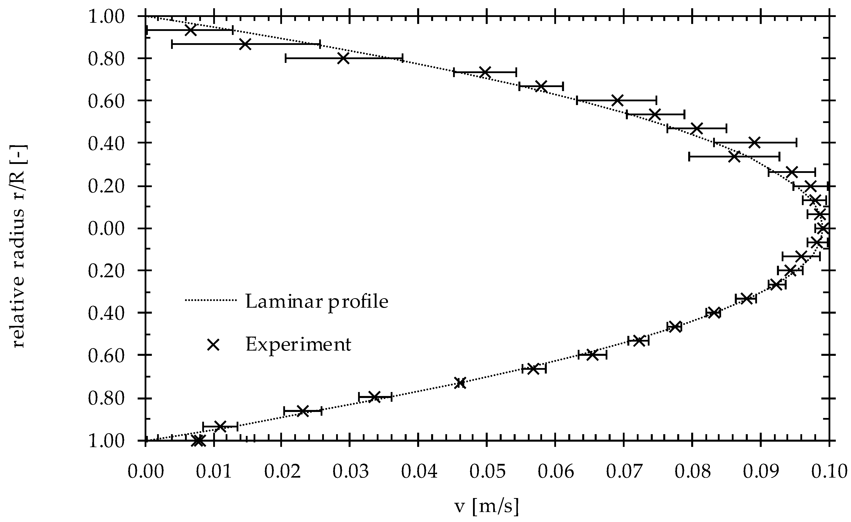
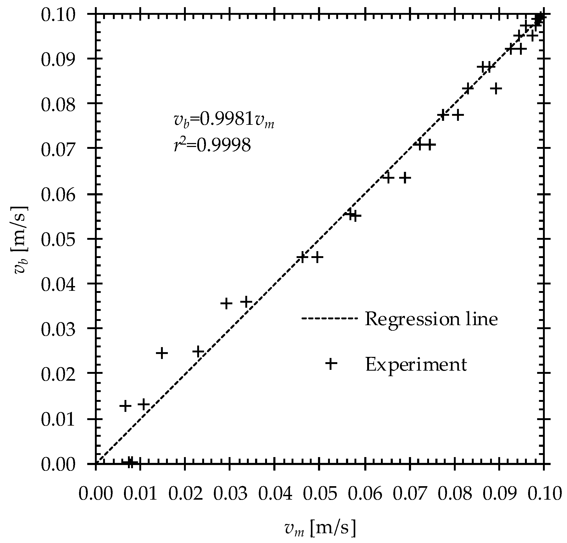
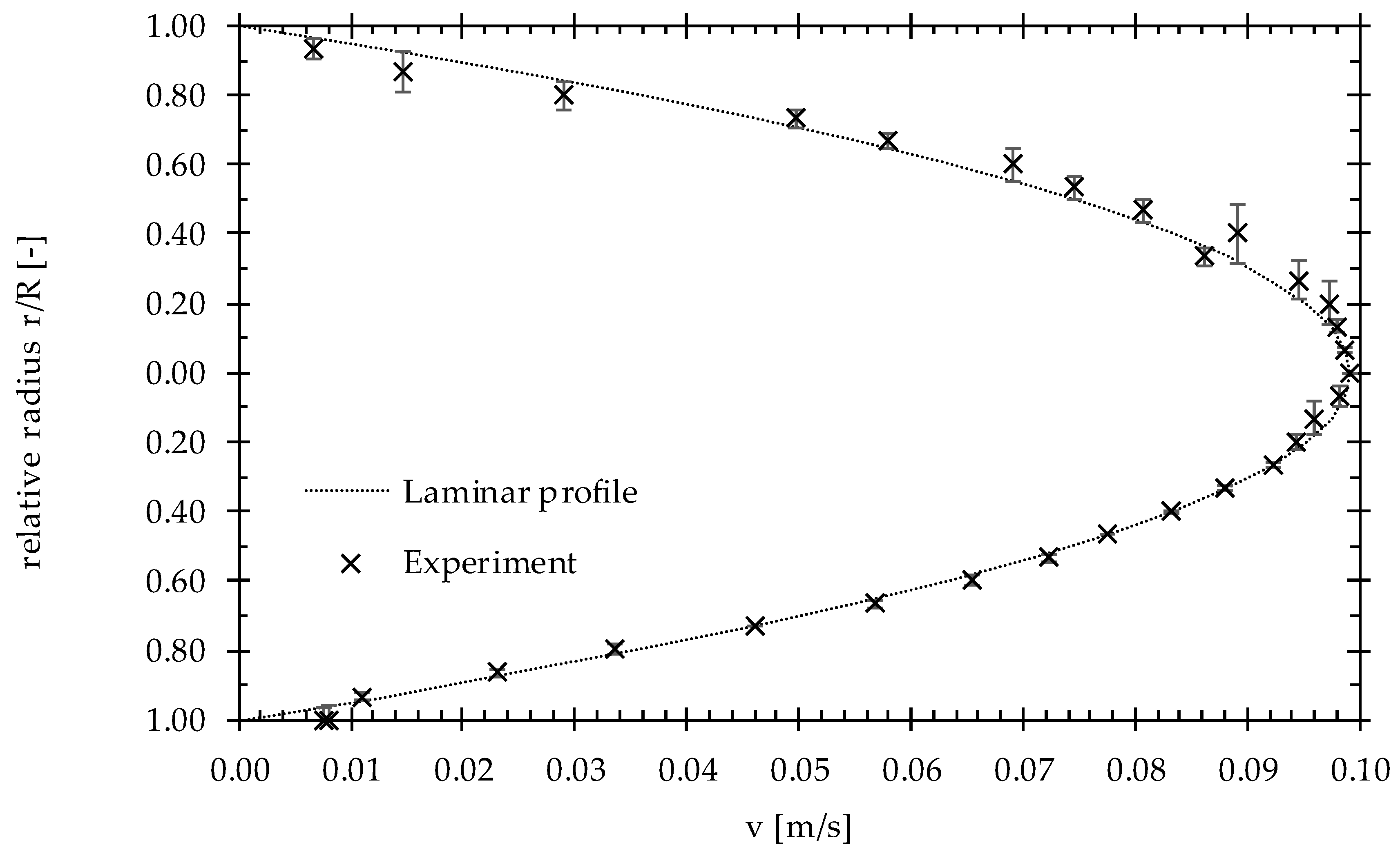
3. Results and Discussion

The researcher adjusts the linear stroke element (8) at the location computed from Equation (18) for each of 31 measurement points along the diameter of the tube (15), and carries out the velocity measurements in these points; then, the researcher repeats the measurement procedure 29 times. Figure 6 shows the velocity profile from the averaged experimental results compared with the benchmark laminar flow for Re = 2137.
To assess quality of the experiments the regression line computed from Equation (23) is plotted in Figure 7 with the Pearson’s coefficient value computed from Equation (24).
The great discrepancies occur in a close vicinity to one tube wall where the velocities in laminar flow vb are close to zero, and the measured velocities vm are about 30 times higher (cf. Figure 7); it may result from the thinner wall in this place, which, unfortunately, may not be checked with the simple measurements because of the long distance from the tube ends.
Figure 8 shows an impact of radial distance determination on the velocity profile measurements; there are plotted vertical errors bars that are the differences between radial distance of the measured velocity and the coordinate of laminar velocity profile. The differences in the first half of the diameter that is closer to the LDA system, which corresponds to the lower part of Figure 8, are significantly less than in the second half beyond the tube axis; the one exception is the first point that was discussed above. The bigger discrepancies arise when the measurement volume approaches the axis, and the maximum is reached 6 mm beyond the tube axis (r/R = 0.4).
The errors in radial distance determination may be caused by other tube thickness in the measurement cross section, such as a non-circular cross section caused by several years of usage in the set-up, inappropriate adjustment of the element of linear stroke, different value of the refractive index, which might have been changed by the seeding particles.
Summarizing the discrepancies, between the benchmark laminar flow profile and the measured velocity profile, are an uncertain combination of the velocity and radial distance determination.

4. Conclusions

For as much as the gradient of the regression line is almost one, and the Pearson’s correlation coefficient is greater than minimal value, which is equal to 0.3557 for 29 degrees of freedom at 95% confidence level, it might be said, in conclusion, that the preliminary experiments are performed in a proper way, and the high quality of the further principal research may be maintained.

Author Contributions

Conceptualization, A.G.; methodology, K.W. and A.G.; validation, K.W. and A.G.; formal analysis, K.W. and A.G.; investigation, K.W.; resources, A.G.; data curation, K.W.; writing—original draft preparation, K.W. and A.G.; writing—review and editing, A.G.; visualization, K.W.; supervision, A.G.; project administration, A.G.; funding acquisition, A.G. and K.W. All authors have read and agreed to the published version of the manuscript.

Funding

The paper was prepared at Students’ Scientific Society “Heat Engineer” at Bialystok University of Technology and were financed by this university. The research was carried out at the Bialystok University of Technology at the Department of HVAC Engineering as the project WZ/WB-IIŚ/4/2019 and was subsidised by the Ministry of Science and Higher Education of the Republic of Poland from funding for statutory R&D activities. The research was conducted using equipment which was purchased thanks to either “INNO—EKO—TECH” Innovative research and didactic centre for alternative energy sources, energy efficient construction and environmental protection—project implemented by the Technical University of Bialystok (PB), co-funded by the European Union through the European Regional Development Fund under the Programme Infrastructure and Environment or “Research on the efficacy of active and passive methods of improving the energy efficiency of the infrastructure with the use of renewable energy sources”—project was co-financed by the European Regional Development Fund under the Regional Operational Programme of the Podlaskie Voivodship for the years 2007–2013.

Institutional Review Board Statement

Not applicable.

Informed Consent Statement

Not applicable.

Data Availability Statement

Not applicable.

Conflicts of Interest

The founding sponsors had no role in the design of the study; in the collection, analyses, or interpretation of data; in the writing of the manuscript, and in the decision to publish the results.

References

  1. IEA. The Future of Cooling: Opportunities for Energy-Efficient Air Conditioning; IEA: Paris, France, 2018. [Google Scholar]
  2. International Energy Agency. OECD Electricity Production by Fuel Type. Available online: https://www.iea.org/data-and-statistics/charts/oecd-electricity-production-by-fuel-type (accessed on 25 March 2021).
  3. Abed, A.M.; Alghoul, M.A.; Sopian, K.; Majdi, H.S.; Al-Shamani, A.N.; Muftah, A.F. Enhancement aspects of single stage absorption cooling cycle: A detailed review. Renew. Sustain. Energy Rev. 2017, 77, 1010–1045. [Google Scholar] [CrossRef]
  4. Álvarez, M.E.; Bourouis, M. Modelling of Coupled Heat and Mass Transfer in a Water-Cooled Falling-Film Absorber Working with an Aqueous Alkaline Nitrate Solution. Energies 2021, 14, 1804. [Google Scholar] [CrossRef]
  5. Asfand, F.; Bourouis, M. A review of membrane contactors applied in absorption refrigeration systems. Renew. Sustain. Energy Rev. 2015, 45, 173–191. [Google Scholar] [CrossRef]
  6. Chan, J.; Best, R.; Cerezo, J.; Barrera, M.; Lezama, F. Experimental Study of a Bubble Mode Absorption with an Inner Vapor Distributor in a Plate Heat Exchanger-Type Absorber with NH3-LiNO3. Energies 2018, 11, 2137. [Google Scholar] [CrossRef] [Green Version]
  7. Suárez López, M.-J.; Prieto, J.-I.; Blanco, E.; García, D. Tests of an Absorption Cooling Machine at the Gijón Solar Cooling Laboratory. Energies 2020, 13, 3962. [Google Scholar] [CrossRef]
  8. Sehgal, S.; Alvarado, J.L.; Hassan, I.G.; Kadam, S.T. A comprehensive review of recent developments in falling-film, spray, bubble and microchannel absorbers for absorption systems. Renew. Sustain. Energy Rev. 2021, 142, 110807. [Google Scholar] [CrossRef]
  9. Lima, A.A.; de NP Leite, G.; Ochoa, A.A.; dos Santos, C.A.; dos Costa, J.A.; da Michima, P.S.; Caldas, A. Absorption Refrigeration Systems Based on Ammonia as Refrigerant Using Different Absorbents: Review and Applications. Energies 2021, 14, 48. [Google Scholar] [CrossRef]
  10. Hartley, D.E.; Murgatroyd, W. Criteria for the break-up of thin liquid layers flowing isothermally over solid surfaces. Int. J. Heat Mass Transf. 1964, 7, 1003–1015. [Google Scholar] [CrossRef]
  11. Bankoff, S.G. Minimum thickness of a draining liquid film. Int. J. Heat Mass Transf. 1971, 14, 2143–2146. [Google Scholar] [CrossRef]
  12. Mikielewicz, J.; Moszynski, J.R. Minimum thickness of a liquid film flowing vertically down a solid surface. Int. J. Heat Mass Transf. 1976, 19, 771–776. [Google Scholar] [CrossRef]
  13. Mikielewicz, J.; Moszynskl, J.R. An improved analysis of breakdown of thin liquid filmse. Arch. Mech. 1978, 30, 489–500. [Google Scholar]
  14. Madejski, J. (Ed.) Theory of Heat Transfer; Technical University of Szczecin Press: Szczecin, Poland, 1998. (In Polish) [Google Scholar]
  15. El-Genk, M.S.; Saber, H.H. Minimum thickness of a flowing down liquid film on a vertical surface. Int. J. Heat Mass Transf. 2001, 44, 2809–2825. [Google Scholar] [CrossRef]
  16. Perazzo, C.A.; Gratton, J. Navier–Stokes solutions for parallel flow in rivulets on an inclined plane. J. Fluid Mech. 2004, 507, 367–379. [Google Scholar] [CrossRef]
  17. Tanasijczuk, A.J.; Perazzo, C.A.; Gratton, J. Navier–Stokes solutions for steady parallel-sided pendent rivulets. Eur. J. Mech. B/Fluids 2010, 29, 465–471. [Google Scholar] [CrossRef]
  18. Ataki, A.; Bart, H.-J. Experimental Study of Rivulet Liquid Flow on an Inclined Plate. In International Conference on Distilation & Absorpiton; GVC- VDI-Society of Chemical and Process Engineering: Baden, Germany, 2002; pp. 1–13. [Google Scholar]
  19. Charogiannis, A.; An, J.S.; Markides, C.N. A simultaneous planar laser-induced fluorescence, particle image velocimetry and particle tracking velocimetry technique for the investigation of thin liquid-film flows. Exp. Therm. Fluid Sci. 2015, 68, 516–536. [Google Scholar] [CrossRef] [Green Version]
  20. Jeong, S.; Garimella, S. Falling-film and droplet mode heat and mass transfer in a horizontal tube LiBr/water absorber. Int. J. Heat Mass Transf. 2002, 45, 1445–1458. [Google Scholar] [CrossRef]
  21. Trela, M.; Mikielewicz, J. Ruch cienkiego filmu w warunkach adiabatycznych. In Ruch i Wymiana Ciepła Cienkich Warstw Cieczy; Burka, E.S., Ed.; Zakład Narodowy im. Ossolińskich Wydawnictwo Polskiej Akademii Nauk: Wrocław, Poland, 1998; p. 391. ISBN 83-04-04474-9. [Google Scholar]
  22. Teleszewski, T.J. Experimental investigation of the kinetic energy correction factor in pipe flow. E3S Web Conf. 2018, 44, 177. [Google Scholar] [CrossRef] [Green Version]
  23. Moffat, R.J. Describing the uncertainties in experimental results. Exp. Therm. Fluid Sci. 1988, 1, 3–17. [Google Scholar] [CrossRef] [Green Version]
  24. Szydłowski, H. (Ed.) Regression. In Theory of the Measurements; Państwowe Wydawnictwo Naukowe: Warszawa, Poland, 1981; p. 267. ISBN 83-01-01843-7. (In Polish) [Google Scholar]
Figure 1. A report of International Energy Agency [2] into monthly electricity production.
Energies 14 03847 g001
Figure 2. Film thickness δ as a function of surface inclination towards the horizon.
Energies 14 03847 g002
Figure 3. The applied setup: 1—intercrossing laser beams, 2—flow explorer with optics system, 3—optical fiber, 4—signal wire to photo-multiplier, 5—The Burst Spectrum Analyzer, 6—the stepper motor controller, 7—x,y,z movement signal wires, 8—the elements of linear stroke along x,y,z axis with spindle drives, 9—personal computer, 10—pump, 11—discharge pipe, 12—upper tank, 13—inlet pipe, 14—straight pipe coupler, 15—transparent tube, 16—valve, 17—temperature meter, 18—outlet pipe, 19—needle valve, 20—float meter, 21—bottom tank, 22—overflow pipe.
Energies 14 03847 g003
Figure 4. A fragment of the horizontal cross-section in the experimental space.
Energies 14 03847 g004
Figure 5. A course of the laser rays from the optics to a measurement point.
Energies 14 03847 g005
Figure 6. A comparison between laminar velocity profile Equation (5) and the experimental results with marked velocity uncertainty.
Energies 14 03847 g006
Figure 7. The plot of the experimental results and regression line Equation (23).
Energies 14 03847 g007
Figure 8. A comparison between laminar velocity profile Equation (5) and the experimental results with marked differences between radial distances.
Energies 14 03847 g008
Publisher’s Note: MDPI stays neutral with regard to jurisdictional claims in published maps and institutional affiliations.

