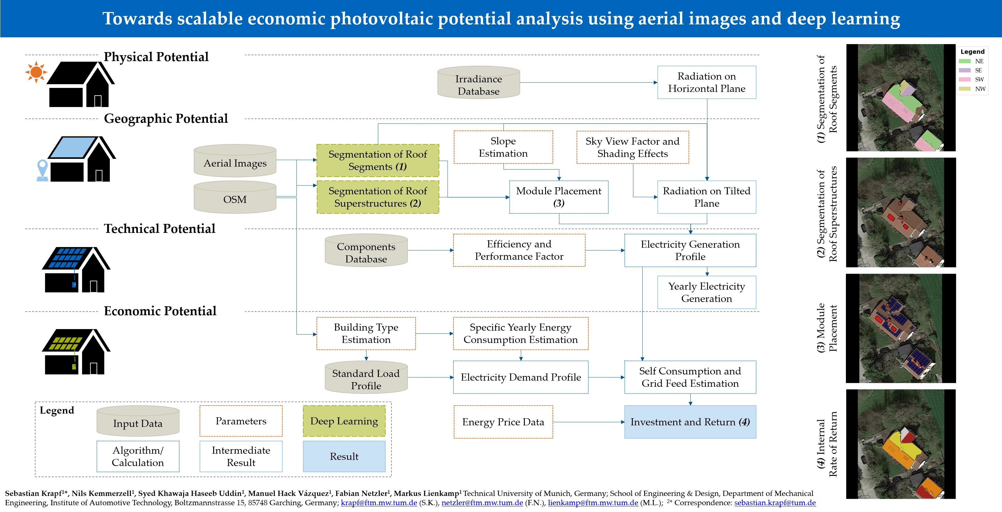
Towards Scalable Economic Photovoltaic Potential Analysis Using Aerial Images and Deep Learning

Abstract

Roof-mounted photovoltaic systems play a critical role in the global transition to renewable energy generation. An analysis of roof photovoltaic potential is an important tool for supporting decision-making and for accelerating new installations. State of the art uses 3D data to conduct potential analyses with high spatial resolution, limiting the study area to places with available 3D data. Recent advances in deep learning allow the required roof information from aerial images to be extracted. Furthermore, most publications consider the technical photovoltaic potential, and only a few publications determine the photovoltaic economic potential. Therefore, this paper extends state of the art by proposing and applying a methodology for scalable economic photovoltaic potential analysis using aerial images and deep learning. Two convolutional neural networks are trained for semantic segmentation of roof segments and superstructures and achieve an Intersection over Union values of 0.84 and 0.64, respectively. We calculated the internal rate of return of each roof segment for 71 buildings in a small study area. A comparison of this paper’s methodology with a 3D-based analysis discusses its benefits and disadvantages. The proposed methodology uses only publicly available data and is potentially scalable to the global level. However, this poses a variety of research challenges and opportunities, which are summarized with a focus on the application of deep learning, economic photovoltaic potential analysis, and energy system analysis.

1. Introduction

The world is increasing efforts to move towards renewable energy production. Solar power is one important pillar in this endeavor for the massive reduction in carbon dioxide emissions. Large-scale, free-standing photovoltaic (PV) plants achieve a low levelized cost of energy (LCOE) and can outperform fossil power plants in this matter [1,2,3]. Though more expensive, rooftop PV systems play a major role in a sustainable energy system because they do not seal additional land area. In the past, the introduction of PV was enabled and accelerated by subsidies. To support policymakers, researchers have conducted rooftop PV potential analyses ranging from city-scale to country-scale. This paper extends existing approaches by presenting a method for a scalable, individual building economic PV potential estimation using publicly available data sources and deep learning approaches. We first present the results and discuss experiences with the implemented methodology to outline challenges and research opportunities in this interdisciplinary field.

1.1. Existing PV Potential Analysis with Respect to Potential Type

PV potential can be divided into physical, geographic, technical, and economic potential, whereas the level of information increases for each type [4,5,6,7,8]. Figure 1 visualizes the PV potential qualitatively.

The physical potential is the solar radiation at a geographic location and consists of direct, diffuse, and reflected radiation of the real-sky global irradiance. PV-GIS [9,10] or the Copernicus Atmosphere Monitoring Service data [11] provide estimations of Europe’s physical potential via Application Programming Interfaces (APIs). Some researchers focus on geographic PV potential, which is the available solar radiation on roofs considering the roof planes’ orientation and shadowing effects of surrounding structures [12,13]. Publications determine the technical potential, which takes the PV system efficiency into account and represents the actual energy generation [5,8,14,15,16,17,18,19,20,21].

The fourth type of potential is the economic potential. Subsidies and policies have major leverage on the economic potential. Furthermore, a positive business case of a PV system is one of the most important drivers for installing PV systems. Therefore, for policymakers, it is important to know the technical potential, but it is even more critical to understand the economic potential. Hence, analyses should be extended from technical potential to economic potential. Recent studies include the economic potential to incorporate only the share of the PV potential, which is economically viable [4,7,22,23,24,25,26,27]. The economic potential can be assessed by the LCOE, a common benchmarking measure for energy generation, which represents the cost per generated kWh over the lifetime of PV systems [28]. A comparison of the generation costs (e.g., LCOE) with an income threshold such as the feed-in-tariffs can determine the economic viability of a PV installation [4,7,22,23]. In addition, publications consider revenue and calculate the return on investment [25,26], the net present value [24], and the payback period [24,25,26,27]. This approach provides a more detailed profitability estimation. It also enables comparing economic potential internationally because it can include different feed-in-tariffs or additional revenue considerations, such as self-consumption models. In Germany, with decreasing feed-in-tariffs, PV systems are increasingly designed for self-consumption purposes and are coupled with stationary battery storages [29]. While it is common for studies on site-level to consider a mix of self-consumption and grid feed-in [29,30,31], few studies, such as the ones from Lee et al. [25,26], consider it on system level.

1.2. Existing PV Potential Analysis with Respect to Method

Besides categorizing publications with respect to potential type, they can also be grouped based on their method for estimating the PV potential. Reviews on methods for PV potential estimation are published by Melius et al. [32] and Freitas et al. [33]. Additionally, a review by Assouline et al. [34] distinguished six types of methods for large-scale PV potential estimation: Physical/empirical, geostatistical, constant values, sampling, Geographic Information System (GIS)/Light Detection and Ranging (LiDAR), and machine learning. The chosen method is strongly dependent on the available data. Therefore, we slightly adapted the categorization from Assouline et al. [34] to integrate the input data perspective. We differentiated four groups with increasing detail of information: statistical, geospatial, aerial image, and 3D. The approaches can also use multiple input data sources. In this case, we assigned the literature to the group with the highest level of detail. The category statistical uses statistical data to estimate the available roof area by assuming roof area per capita. Furthermore, the effects of roof orientation, shadow, or roof superstructures are considered using constant factors. Statistical approaches often examine large study areas such as the European Union [21,35] or Brazil [23] and take a top-down perspective. The geospatial approach determines available roof areas based on geospatial vector data such as building cadasters or maps. Hence PV potential is estimated bottom-up. Those studies applied constant factors to account for decreasing PV potential due to shadow and superstructures. The study areas are typically larger, such as Spain [8], the Canary Islands [22], or the Fujian Province [24].

With the availability of 3D models, PV potential can be assessed with higher accuracy and a higher resolution. Three-dimensional models usually contain buildings on the city level and can be created using stereo photos or LiDAR. The approaches using existing semantic 3D city models based on the CityGML standard [36] were also explored [37,38]. Studies on the city level were conducted for Feldkirch [13], Lisbon [14], Uppsala [20], Cambridge [39], and the Chao Yang District in Beijing [40], among others [12,15,38]. Hong et al. presented a 3D method for potential technical estimation of the Gangnam district in Seoul, which included a hill shade analysis based on geospatial vector shapes of building and elevation information [17]. Lee et al. extended the results with a potential economic analysis [25]. Margolis et al. [16] analyzed 128 cities in the USA using LiDAR data. Gagnon et al. [41] expanded this study to the whole USA by statistically extrapolating the results of the 3D approach. Other mixed approaches were presented by Assouline et al. in several publications [18,42]. The authors used 3D data and machine learning methods to extrapolate the technical potential estimated with high detail data from Geneva to the whole of Switzerland. A study for Switzerland by Walch et al. [5] used a similar approach and determined its uncertainty.

The LiDAR-based 3D approaches can be considered the best methods with regard to the level of detail of the input data [34]. Furthermore, they can be coupled with machine learning methods such as random forests to extrapolate findings from a smaller to a larger study area. This combination shows high accuracy and relatively low computational time [5,42]. The examples of existing LiDAR-based solar cadasters were made available in recent years by Mapdwell [43], Google’s Project Sunroof [44], or tetraeder.solar [45]. However, even though LiDAR data are becoming increasingly available, there is still no exhaustive coverage. Therefore, some researchers propose alternative methods for extracting roof information based on aerial images.

The task of roof segment segmentation was investigated outside of the context of PV potential analysis. For example, Hazelhoff [46] used a line detection approach [47] to detect the roof ridge and gutters. Fan et al. used image processing methods to determine roof planes from LiDAR data [48]. Merabet et al. [49] presented a building roof segmentation method that is based on the watershed segmentation technique.

To estimate the technical PV potential of the city of Turin, Bergamasco et al. [19] explored a methodology that extracts roof segments by clustering an image’s pixels into bins based on their color tones. Their qualitative validation revealed an accuracy level of around 90% for their dataset. Mainzer et al. [7] assessed the economic potential of the city of Freiburg. They used image processing to detect roof ridges and roof outlines and estimate the azimuth correctly for over 70% of the roofs. Additionally, the authors proposed an approach based on contour detection [50] to identify roof superstructures that decrease the usable roof area. Furthermore, they used convolutional neural networks (CNN) to identify existing PV modules. The reported accuracy reaches over 90% on their dataset, indicating the high potential of CNNs for this task [7].

In recent years, deep CNNs outperformed the state-of-the-art in many image-recognition tasks [51]. Therefore, deep learning has gained significant relevance in the remote sensing field [52]. For example, CNNs were successfully used for the task of building footprint segmentation [53,54]. In the PV context, studies exploited the advances in deep learning for image recognition tasks. One application of CNNs is the mapping of existing solar modules by semantic segmentation. Yu et al. [55] constructed a solar deployment database for the USA using their developed deep learning framework DeepSolar. Mayer et al. extended the DeepSolar framework to Germany and applied it to the German state of North Rhine-Westphalia [56]. Castello et al. [57] demonstrated the applicability of CNNs for mapping PV modules in Switzerland. Furthermore, CNNs are used for the estimation of available roof areas. A study from Huang et al. [58] estimated the geographic potential of Wuhan, China using semantic segmentation of roof footprints. The authors only detected the whole roof and did not consider individual roof segments and their orientation. To the best of our knowledge, the DeepRoof project presented by Lee et al. [59] is currently the only publication that extracted roof segments, including their azimuth values, from aerial images using CNNs. The authors labeled their own dataset containing 2274 buildings from six US cities. The comparison of their 2D approach for potential technical estimation with the LiDAR-based Google Project Sunroof results [44] demonstrates small mean errors of the estimated available PV installation area. This indicates that the PV potential analysis using deep learning and aerial images has a great potential to be a viable, scalable alternative to 3D LiDAR methods.

1.3. Contributions of the Paper

The literature analysis shows that currently, only a few publications consider the economic PV potential. Furthermore, the state-of-the-art bottom-up approaches are based on 3D data, with the drawback of fragmentarily available data. Hence, this paper combines the latest scientific developments and proposes a methodology for bottom-up economic PV potential analysis using aerial images and deep learning. To the best of our knowledge, there is currently only one paper that used aerial images and deep learning to extract roof segments for PV potential analysis [59]. This paper applies the same approach and adds to the state of the art by exploring the application of deep learning for the task of roof superstructure segmentation. The methodology only relies on publicly available data, making it potentially scalable on a global level. The potential economic assessment calculates the internal rate of return (IRR) instead of LCOE, which contains more information due to revenue and cost considerations. This paper’s contributions are:

• A methodology for scalable, bottom-up, economic PV potential analysis using aerial images and deep learning as well as publicly available data;
• The application of CNNs for semantic segmentation of roof segments and roof superstructure. Initial results are discussed to point out the advantages and disadvantages of the methodology;
• A comprehensive summary of research challenges and opportunities for this novel approach.

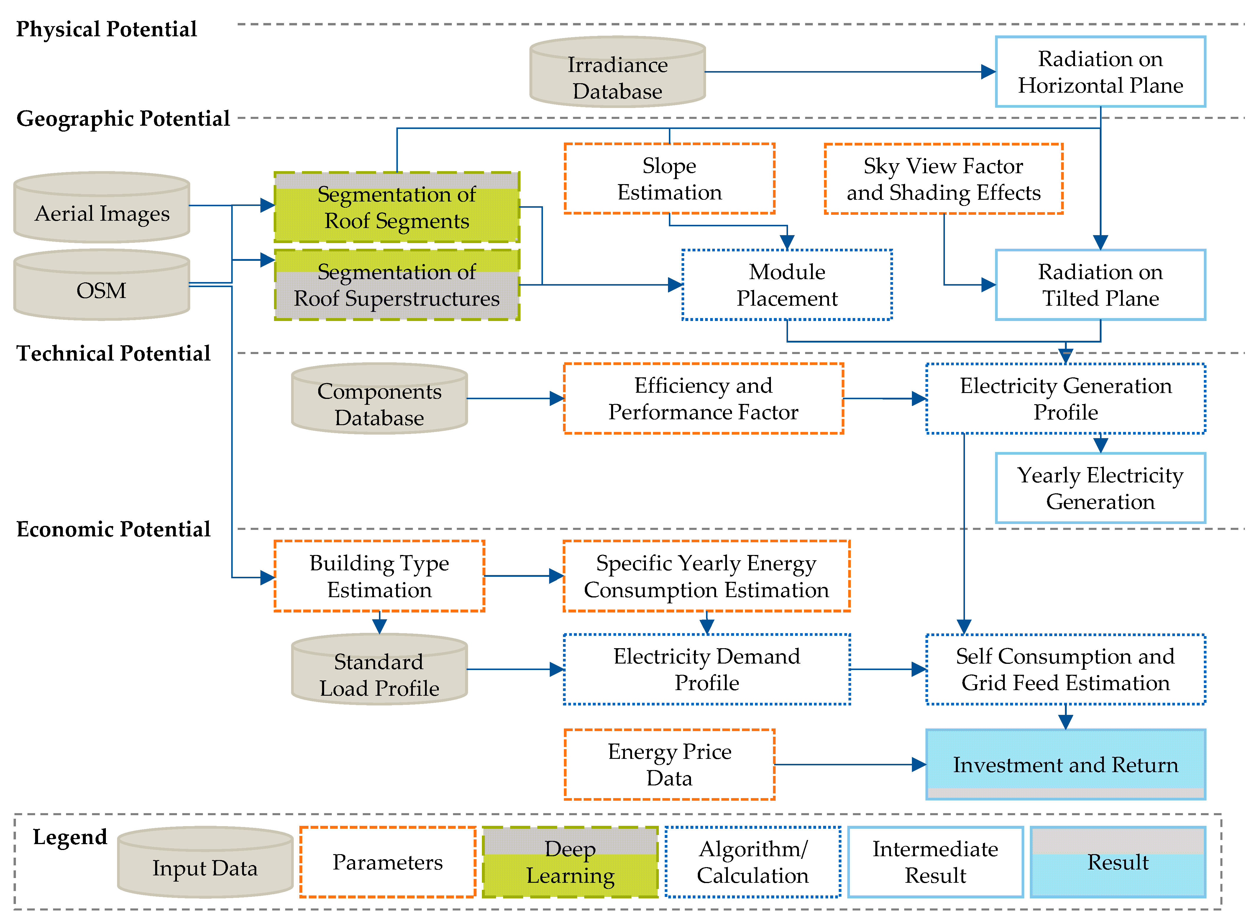
2. Materials and Methods

This section describes the methodology for the scalable, large-scale economic PV potential analysis based on aerial images and deep learning. Figure 2 visualizes the respective steps grouped by the four potential types. The input data mainly rely on public data from Copernicus [11], Open Street Maps (OSM) [60], technical specifications of PV systems, as well as aerial images accessed from google maps static API [61]. Furthermore, some steps require input parameters that have been derived from the literature or online sources. The core element of deep learning-based extraction of roof information from aerial images is highlighted in green in the Section 2.2. The other data processing steps use simple algorithms or calculations and are open for expansion in the future. Each potential type is calculated as an intermediate result and consecutively used to estimate the final result, the economic potential in the form of the IRR.

2.1. Physical Potential

This paper’s approach used data of solar radiation on the horizontal plane from the Copernicus Atmosphere Monitoring Service [11]. The radiation data were provided with a continuous spatial resolution by interpolation [62]. We downloaded the data for one representative location in the small study instead of each individual roof. This simplification is viable because of the neglectable variance of the radiation within the small study area.

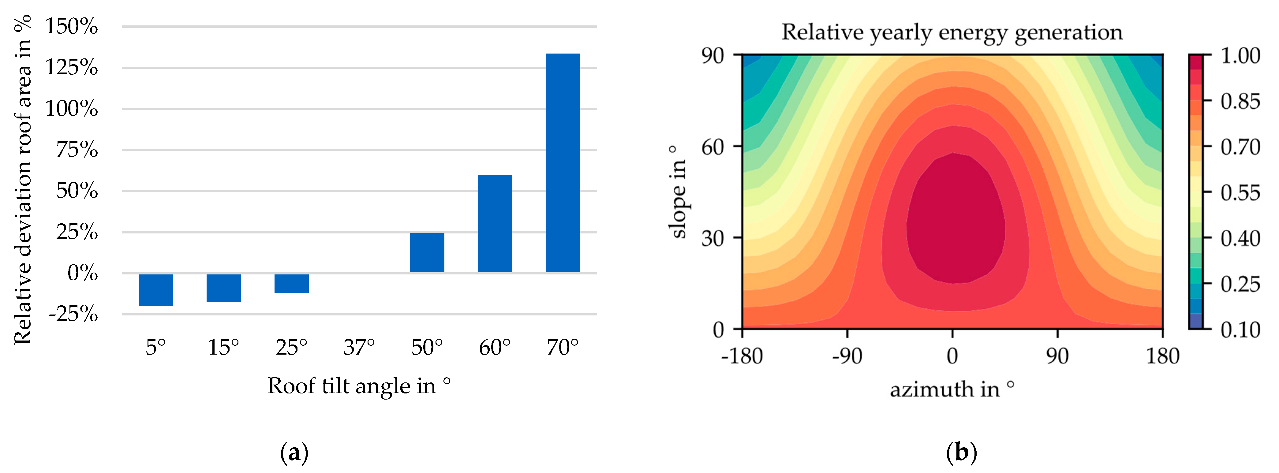
2.2. Geographic Potential

As described in the overview of this paper’s contributions, a novel approach for determining the geographic potential based on aerial images is presented.

First, we requested all building footprints of a study area from OSM [60] to create a list of buildings for the potential analysis. By this, we avoided analyzing areas without buildings, and we made sure to cover all mapped roofs. Although OSM offers high completeness and spatial accuracy of 1.5 m [63], incorrect map data can lead to misestimations of the potential on aggregated city level. Alternatively, other map services with higher data quality could be used. Furthermore, a CNN trained for building footprint segmentation could supply a tailored roof object list. The second input data source is the Google Maps static API [64] which provides the aerial images with a resolution of up to 0.15 m/px [61]. High-resolution imagery is a prerequisite for detecting relatively small roof superstructures.

The input data are used for the semantic segmentation of roof segments and roof superstructures. The CNNs’ outputs are further processed to pass roof segment polygons, their orientation, and the respective superstructure polygons to the module placement algorithm. On inclined roof segments, the modules are projected onto the horizontal plane as a function of the tilt angle, assuming an orthogonal aerial image. Then, a grid of modules is placed onto the segment aligning its longest side. Finally, modules intersecting with superstructure are deleted. On flat roofs, the placement has more degrees of freedom. Modules can be oriented south, east, west, or aligned with the building. On flat roofs, space for maintenance or fire protection is considered. The usable area is the sum of all successfully placed modules.

A critical factor for the module placement and the calculation of the irradiation is the inclination angle of the roof. Its inference from 2D image data provides a serious challenge due to missing height information. To cope with this problem, the slope angle is determined statistically using a normal distribution with a mean of 37° and a standard deviation of 15° as proposed by Mainzer et al. [7]. Hereby, the same angle is assumed for all roof segments of the same building. This assumption holds true, especially for gabled roofs, which are very common in Germany, but also for hip and pyramid roofs. However, more complex roof types may deviate from this assumption. Flat roofs are recognized by the CNN. The statistical slope estimation leads to the erroneous calculation of the available roof area and the irradiation on the roof. Figure 3 shows the relative deviation of the roof area and the yearly energy generation compared to a 37°, south-facing roof. While the difference of a 5° to a 37° tilted area is only 20%, the error becomes large for higher slopes. A 70° slope would mean a deviation of more than 125% from the 37° area. The effect of the slope on the irradiance on a tilted surface is visualized by the relative yearly energy generation. A 60° tilted, south-facing PV module yields around 5% less energy than a 37° module. This effect becomes larger for east- or west-facing roofs, where this difference is around 10%. The use of statistical slope estimation results in a higher variance of PV system configurations but also leads to greater deviations from the real PV potential, especially if a flat roof is assigned with a high slope value and vice versa. This approach could be improved by adding limiting the slope range with respect to additional roof information such as building type or roof area. For example, this could avoid assigning high slope values to industry or larger office buildings.

The solar irradiation on a tilted surface is calculated for each roof segment. It is split into a direct, diffuse, and ground-reflected component. The direct and ground-reflected components are calculated using isometric approaches, which rely on the trigonometric relationship between the radiation beams and the roof surface. We applied the model by Perez et al. [65] to calculate the diffuse radiation component using pvlib [66]. It has shown high accuracy in comparison to other models [67]. Hence, it was already used in connection with PV potential analysis [39,68,69]. Shadowing effects and reduced sky view factors pose the same challenge as the slope estimation. This is considered with a constant value of 15%, whereas in the literature, values between 15% and 30% were applied [19,70,71,72,73]. It was applied to the whole PV system and not to each module individually.

In the next sections, the core steps of this paper, the semantic segmentation for roof information extraction, are described in more detail.

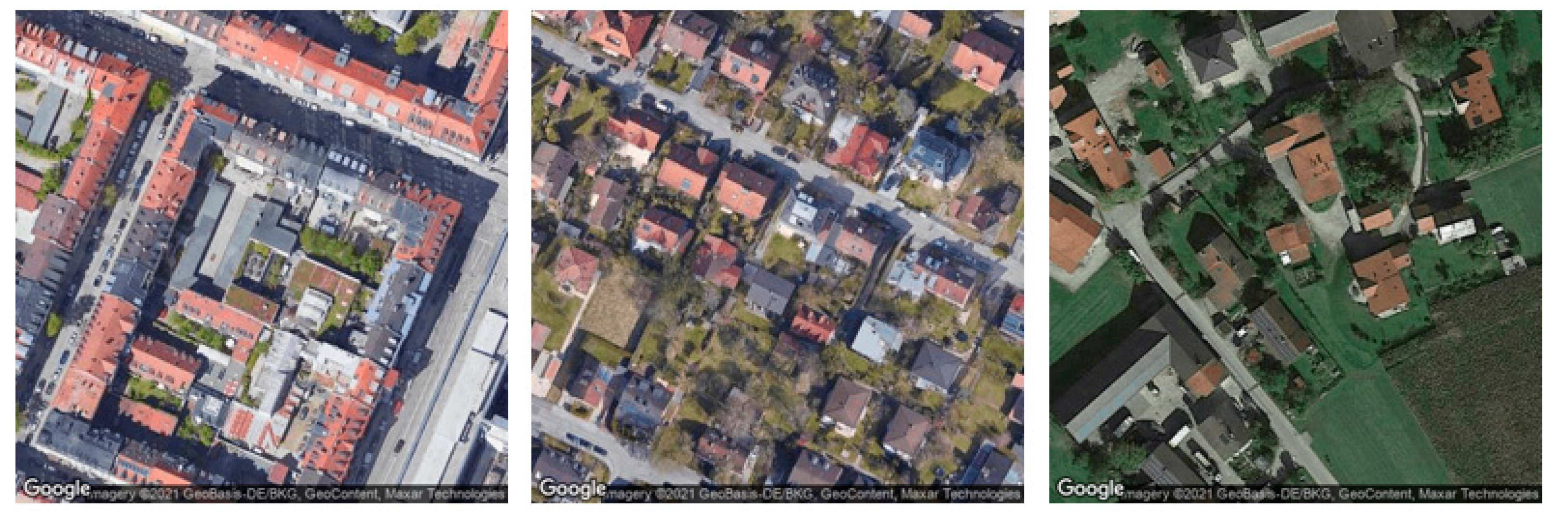
2.2.1. Datasets for Semantic Segmentation

CNNs benefit from large training datasets. In the remote sensing context, such datasets exist, for example, for building footprints [74,75] or existing PV modules [76]. Lee et al. published a smaller dataset consisting of 444 images and 2274 buildings along with the DeepRoof paper [59]. We used this data in this paper for the roof segment training. There are 20 different label classes, including 16 for azimuth directions, as well as one for flat roofs and domes, respectively. Each azimuth class, e.g., north, covers a span of 22.5 degrees. An additional label classifies nearby trees. Pixels that do not belong to any class are labeled as background. Currently, to the best of our knowledge, there is no label dataset for roof superstructures. Therefore, we created our own preliminary dataset from aerial images of a small municipality in Bavaria, Germany. A total of 407 images with a size of 512 × 512 pixels were annotated as polygons with six semantic superstructure classes: window, dormer, chimney, ladders, PV modules, and unknown/others.

2.2.2. Performance Evaluation of Semantic Segmentation

This paper uses the Intersection over Union (IoU) or Jaccard Index for evaluating the semantic segmentation result, as it is the most commonly used metric [77]. This IoU measures the fraction of the intersection of the actual and predicted values to the Union for a specific class.

$$\mathrm{IoU}=\frac{\mathrm{Area}\mathrm{of}\mathrm{overlap}}{\mathrm{Area}\mathrm{of}\mathrm{Union}}$$

(1)

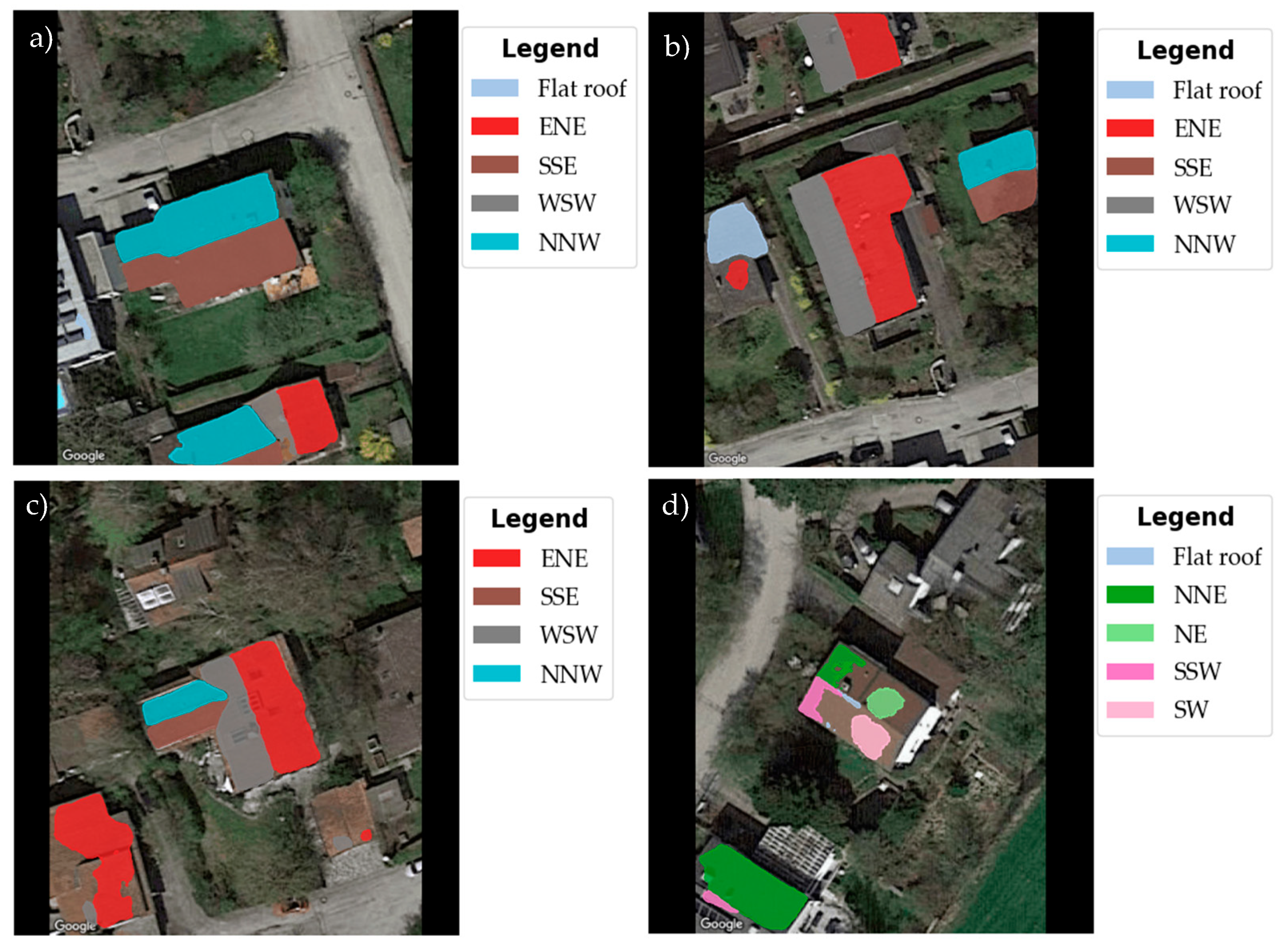
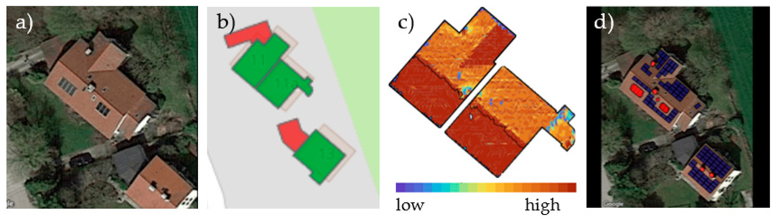
2.2.3. Semantic Segmentation for Roof Segments

The first semantic segmentation step is the identification of individual roof segments and their orientation, similarly to Lee et al. [59]. For this purpose, we train a CNN using a U-Net architecture [78] with a ResNet−152 [79] backbone. The DeepRoof dataset is randomly split into 60% training, 20% validation, and 20% test data. To increase the size of the dataset, each image is rotated by 30 degrees 12 times. The training is performed in two stages. At first, the weights of the encoder are frozen, and only the decoder weights are optimized using Adam optimizer [80]. The stage lasts for 55 epochs at 66 iterations and a batch size of 64 images. The learning rate starts at 4 × 10⁻⁴ and is divided in half after 40 epochs. The second training phase incorporates all existing weights lasting for 100 epochs. It starts at a learning rate of 4 × 10⁻⁵ which is divided in half after 60 and 80 epochs, respectively. During the training process, random augmentations are applied to the images to artificially increase the dataset and make the network less prone to overfitting [81]. The augmentations can be split into three different categories, which can be applied at the same time. Initially, the image is mirrored on the horizontal or vertical center axis. Afterward, the image can be randomly cropped to 80% of its size. Lastly, the image is changed on a pixel level by varying its brightness, contrast, gamma, or saturation. On the test set, we achieve an IoU of 0.89 averaged over all classes and 0.84 only focusing on roof classes.

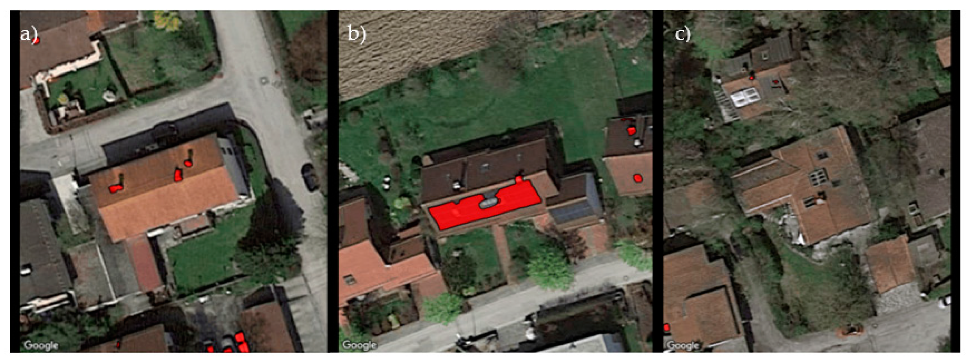
2.2.4. Semantic Segmentation for Roof Superstructures

The second semantic segmentation step uses a deep learning approach for roof superstructure segmentation, which is inspired by the PV mapping approaches [55,56,57]. A CNN based on the U-Net is used because of its superior performance on small datasets [78]. We compared the backbone architectures EfficientNet-B3 [82], Inception-resnet-v2 [83] and VGG-19 [84]. We chose Inception-resnet-v2 because of better performance. Due to the small size of the dataset with only 407 images, a split of 86%, 7%, and 7% was used for training, validation, and testing, respectively. Mirroring and cropping were applied to the superstructure dataset, similarly to the roof segments dataset augmentation. Furthermore, we merged all six superstructure classes into one superstructure class. In general, it would be preferable to detect each superstructure class individually, which leads a more challenging training.

The network is trained with an initial learning rate of ${10}^{-4}$. The learning rate is decreased using an exponential decay rate scheduling. We initialized the weights applying He initialization, which is the preferred choice for ReLU activated neural networks [85]. The Adam optimizer is used for the training process and a dropout with a skip probability of 0.5 is conducted after each layer [80].

Figure 4 visualizes the class representation of roof pixels, superstructure pixels, and background pixels. All six superstructure classes combined make up only 1.44% of all pixels. Jadon [86] provided an overview of loss functions for semantic segmentation and recommended the use of Focal Loss for highly imbalanced classes. Therefore, we implemented a combination of Focal Loss with weighted Dice Loss. This led to better performance than the Cross-Entropy Loss function.

2.3. Technical Potential

The technical potential is the electricity generation considering losses caused by the technical properties of the solar system (

Table A1. Equations for technical and economic potential calculation.

Calculation of the Technical Potential
Physical Potential	$E_{phy}=I_{hor,glob}=I_{hor,dir}+I_{hor,diff}$
Geographic Potential	$E_{geo}=I_{tilt,eff} A_{usable}N{F}_S$
Global Irradiation on Tilted Surface	$I_{tilt,glob}=I_{tilt,dir}+I_{tilt,diff}+I_{tilt,Ground}$
Effective Irradiation on Tilted Surface	$I_{gen,eff}=I_{gen,glob} U_{irr}$
Module Area on a Tilted Surface	$A_{mod,proj}=w_{Module} l_{Module} \cos {\theta }_T$ $A_{usable}=n A_{mod,proj}$
Technical Potential	${\mathrm{E}}_{\mathrm{tech}}=E_{geo} {\eta }_{Module} PR$
Calculation of the Economic Potential
Investment Costs	$C_{Invest}=\left(P_{PV,max} c_{pv}\right) \left(1+VAT\right)$
Maintenance Costs	$C_{Maint}={\displaystyle {\displaystyle \sum }_{t=1}^T}\left(C_{Maint,fix}+P_{PV,max}{c}_{Maint,var}\right) {\left(1+i_{inf}\right)}^t {\left(1+i\right)}^{-t}$
Weighted Average Cost of Capital	$WACC=\frac{Equity}{Equity+Debt} i_{Equity}+\frac{Debt}{Equity+Debt} i_{Debt}$
Self-Consumption Ratio	$sc\left(t\right)=\frac{E_{sc}\left(t\right)}{E_{tech}\left(t\right)}$
Fed-In Electricity Within One Year	$E_{Feed-in}={\displaystyle {\displaystyle \sum }_{t=1}^{N_{Year}}}\left(1-sc\left(t\right)\right) E_{tech}\left(t\right)$
Self-Consumed Electricity Within One Year	$E_{sc}={\displaystyle {\displaystyle \sum }_{t=1}^{N_{Year}}}sc\left(t\right) E_{tech}\left(t\right)$
Net Present Value	$NPV=R_{Feed-in}+R_{sc}-C_{Invest}-C_{Maint}-C_{EEG}$
Revenues from Feed-In	$R_{Feed-in}={\displaystyle {\displaystyle \sum }_{t=1}^T}{E}_{Feed-in} e_{tariff}{\left(1-b\right)}^t {\left(1+i\right)}^{-t}$
Revenues from Self-Consumption	$R_{sc}={\displaystyle {\displaystyle \sum }_{t=1}^T}{E}_{sc} p_{Electricity} {\left(1+\Delta p_{Electricity}\right)}^t {\left(1-b\right)}^t {\left(1+i\right)}^{-t}$
EEG-levy (Levy for self-consumption in Germany)	$C_{EEG}=\{\begin{array}{ll}0,& P_{PV,max}<10kWp\\ {\displaystyle {\displaystyle \sum }_t^T}0.4E_{sc}{c}_{eeg}{\left(1+\Delta c_{eeg}\right)}^t {\left(1+i\right)}^{-t},& 10kWp\le P_{PV,max}\le 750 kWp\\ {\displaystyle {\displaystyle \sum }_t^T}{E}_{sc} c_{eeg}{\left(1+\Delta c_{eeg}\right)}^t {\left(1+i\right)}^{-t},& else\end{array}$

). Following [87], the framework differentiates between the technical efficiency of the single module and the performance ratio on the plant level. The efficiency is a unique characteristic of a certain module type. In contrast, the performance ratio is a constant factor that comprises multiple aspects reducing the power output of the entire solar plant. It considers losses from dirt, turndown, temperature dependencies, partial load operation, conduction losses, and shadowing effects. Quaschning [87] proposed a performance ratio of 0.7. Instead, we used a performance ratio of 0.8 (

Table A3. Summary of technical assumptions.

Factor	Variable	Value
Module Placement on Flat Roofs		South-Orientation
Area Usage on Flat Roofs	F	1:2
Module Slope on Flat Roofs	-	36°
Shadow Utilization Factor	$N{F}_S$	0.85
Performance Ratio	$PR$	0.80
Module Peak Power	$P_{module}$	300 Wp
Efficiency	${\eta }_{module}$	20.0%
Module Length	$l_{module}$	1650 mm
Module Width	$b_{module}$	992 mm

) because we considered shadowing losses separately in the geographic potential.

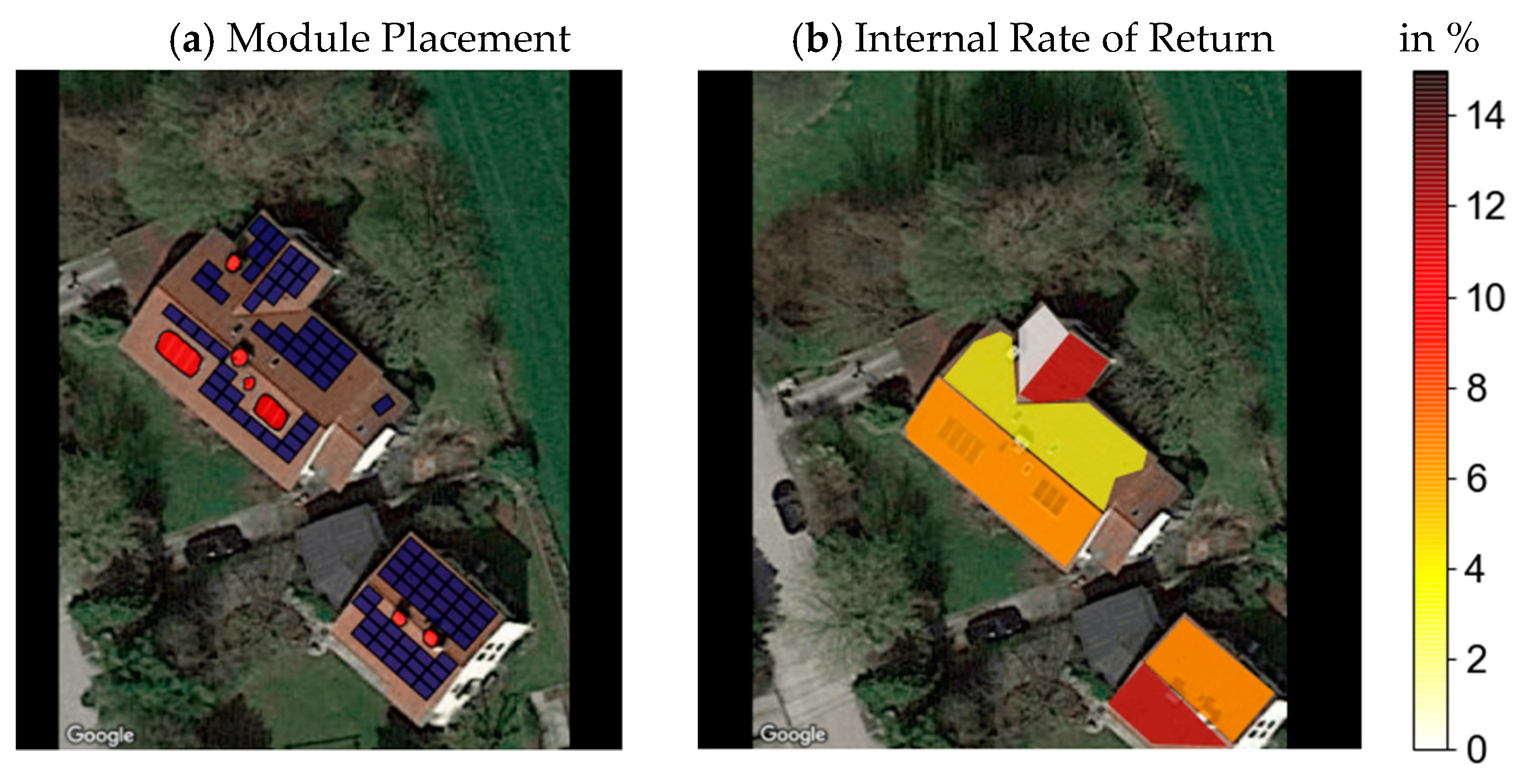
2.4. Economic Potential

This paper extends existing economic potential estimations [7,23] from LCOE to net present value. In addition to costs, the approach includes savings and revenues and thus has more explanatory value than LCOE. However, it requires estimating the electricity consumption of buildings.

The first step is extracting building types from OSM building tags. We differentiated between residential, industrial, commercial, and public buildings because of their specific electricity consumption characteristics and electricity prices. According to standard load profiles for German buildings [88], commercial buildings exhibit their peak load at noon; meanwhile, residential consumption peaks in the morning and evening. Additionally, commercial energy prices are lower than residential ones. The load profile of the building is determined by applying the methodology of Alhamwi et al. [89]. The yearly energy consumption is estimated by multiplying the building area with the specific consumption per square meter. Consequently, standard load profiles [88] are used to obtain a consumption time series.

Following Bertsch et al. [90], the economic return of a solar plant is calculated using the IRR. The share of self-consumption and grid feed is calculated dependent on the technical potential and energy consumption. The revenues differ between the two cases. The feed-in tariff stays constant over the entire lifetime of the plant while the electricity price increases based on historical data [21], which makes self-consumption even more attractive. The costs are divided into initial investment costs and yearly maintenance costs. Additionally, the fee on self-consumption for larger PV systems can be considered (Table A1). The economic potential can be described as the share of technical potential for which the IRR exceeds a given threshold. This publication uses the weighted average cost of capital as the threshold.

2.5. Case Study and Parameterization

In this paper, we conducted a case study to discuss the applicability of the proposed method. The method analyzes each building individually and takes 1–2 min per building on a laptop with an Intel i7-7820HQ processor. Scaling this building-specific analysis to a whole city or region would require optimization of the program. The computation can be parallelized well to decrease the overall runtime. We selected a small residential area as a case study and chose the town Grafing bei München, because of the availability of potential solar information from a LiDAR-based cadaster [91]. The number of buildings was limited to 71 to allow for manual in-depth examination and comparison. The suburban setting was chosen because of the similarity to the training data. The equations for the technical and economic calculations are given in Table A1 and

Table A2. Overview of variables used for technical and economic potential calculation.

Variable	Unit	Description	Variable	Unit	Description
$A_{mod,proj}$	m²	Projected Horizontal Module $A=\pi r^2$	$\mathrm{ev}$	-	Self-Consumption Rate
$A_{usable}$	m²	Area all Modules on Segment	$Debt$	€	Debt
$b$	-	Degradation Rate	$h$	-	Hurdle Rate
$w_{Module}$	m	Module Width	$I_{tilt,Ground}$	kWh/m²	Ground-Reflected Irradiation on a Tilted Surface
$C_{Maint}$	€	Maintenance Costs	$I_{tilt,diff}$	kWh/m²	Diffuse Irradiation on a Tilted Surface
$C_{Maint,fix}$	€	Fix maintenance Costs	$I_{tilt,dir}$	kWh/m²	Direct Irradiation on a Tilted Surface
$c_{Maint,var}$	€/kWp	Variable maintenance Costs	$I_{tilt,eff}$	kWh/m²	Effective Irradiation on a Tilted Surface
$C_{EEG}$	€	Costs from EEG Levy	$I_{tilt,glob}$	kWh/m²	Global Irradiation on a Tilted Surface
$C_{Invest}$	€	Investment Costs	$I_{hor,diff}$	kWh/m²	Diffuse Irradiation on a Horizontal Surface
$c_{eeg}$	€/kWh	EEG Levy	$I_{hor,dir}$	kWh/m²	Direct Irradiation on a Horizontal Surface
$\Delta c_{eeg}$	-	Yearly Change EEG Levy	$I_{hor,glob}$	kWh/m²	Global Irradiation on a Horizontal Surface
$c_{pv}$	€/kWp	Specific Investment Costs	$i$	-	Internal Rate of Return
$E_{sc}$	kWh	Self-Consumption	$i_{Equity}$		Interest Rate (Equity)
$E_{Feed-in}$	kWh	Feed-In Electricity	$i_{Ebt}$		Interest Rate (Debt)
$E_{geo}$	kWh	Geographic Potential	$i_{inf}$	-	Inflation Rate
$E_{eco}$	kWh	Economic Potential	$NPV$	€	Net Present Value
$E_{phy}$	kWh/m²	Physical Potential	$l_{Modul}$	m	Length of pv Module
$E_{tech}$	kWh	Technical Potential	$VAT$	-	Value Added Tax
$E_{Consumption}$	kWh	Electricity Consumption	$U_{irr}$	-	Utilization Factor Irradiation
$Equity$	€	Equity	$P_{PV,max}$	kWp	Plant Size
$e_{Tariff}$	€/kWh	Feed-In Tariff

of Appendix A. Appendix B also summarizes technical and economic assumptions in Table A3 and

Table A4. Summary of economic assumptions.

Factor	Variable	Value	Source
Specific Investment Costs (incl. Value-added tax, VAT)	$c_{pv}$	1071 €/kWp	[3] + VAT
Maintenance Costs Variable	$c_{Maint,var}$	22.50 €/kWp	[3,100]
Maintenance Cost Fix	$C_{Maint}$	100.00 €	[3,100]
Electricity Price	$p_{Electricity}$	30 ct/kWh	Assumption
Yearly Change of Electricity Price	$\Delta p_{Electricity}$	2.0%	Assumption
Feed-In Tariff up to 10 kWp	$e_{feed-in}$	7.81 ct/kWh	[101]
Feed-In Tariff up to 40 kWp	$e_{feed-in}$	7.59 ct/kWh	[101]
Feed-In Tariff up to 100 kWp	$e_{feed-in}$	5.95 ct/kWh	[101]
EEG-Levy	$c_{eeg}$	6.50 ct/kWh	[102]
Interest Rate Equity	$i_{Equity}$	6.0%	[103] (p 159)
Interest Rate Debt	$i_{Debt}$	2.0%	[104]
Debt Ratio	$l$	80.0%	[3]
Inflation Rate	$i_{inf}$	1.5%	Assumption
Degradation	$b$	0.25%	[105,106]
Time Horizon	$T$	20a	[3,107,108]

.

3. Results and Discussion

3.1. Results Convolutional Neural Networks

The IoU of the trained networks for semantic segmentation of roof segments and roof superstructures are 0.84 and 0.64, respectively. These values are in the range of similar other publications, the DeepRoof paper [59] for roof segmentation and a paper on PV module detection [57]. However, these values represent preliminary results and cannot be used as a benchmark. In deep learning, the selection or variation of the training, validation, and test data induce significant effects on the training results. Within the scope of this paper, we did not carry out a deeper analysis of those effects. Therefore, the next sections focus on qualitative discussion of example images within the study area.

The roof segmentation is a critical step in the methodology because the rest of the PV potential analysis is based on the roof geometry. Figure 5 presents four examples of the resulting roof segments for the selected case study area. Examples (a) and (b) show a correct segmentation result. The buildings in the center are covered entirely by two segments. Most of the surrounding building area is detected as well. The azimuth classes of the segments are correctly labeled. In Figure 5a, a small part of a flat roof remains undetected. In Figure 5b, the roof segment of the building in the left-center was labeled with two classes, but only the east–north-east (ENE) azimuth would be correct. Figure 5c displays a mediocre result. The center building is more complex than the gable roofs of (a) and (b) and was segmented well. Both coverage and azimuth classes are correct. However, the surrounding buildings were detected only partly or not at all. Possibly because of trees covering parts of the roof. The last Figure 5d shows a building with incorrect results, although gabled roof structures are usually detected well. The network proposes five different classes instead of two, and the roof is not covered well. A possible explanation could be the ladder on the roof, which could be interpreted as a separating line between two buildings. The building in the upper right is not detected at all. The results confirm the potential of using deep learning PV potential analysis demonstrated by the DeepRoof paper [59]. However, the number of misclassified buildings is still too high to estimate the PV potential for a whole area with the high accuracy of each individual building. Additional training for the roof segmentation network or quality control would be required.

The second CNN was trained to detect roof superstructures. We trained the network on a single superstructure class, as well as on multiple classes such as windows, PV modules, chimneys, and dormers, and achieved better results for the single class training. Figure 6 exhibits examples.

Figure 6a shows a correct semantic segmentation for the center building. A superstructure of the top-left building is also detected. The network labeled superstructures in the bottom, which are parked cars. The network is also able to detect existing PV modules as superstructures, as displayed in Figure 6b. However, additional modules on the smaller building attachment are not recognized. Further superstructures on the center building, such as the chimney or windows, remain unlabeled. Figure 6c shows the same building as Figure 5c. There are five superstructures on the center roof, but none of them are detected. Similar to the roof segmentation network, the superstructure segmentation network indicates the potential for correctly labeling obstructions on the roof.

3.2. Results Economic Potential

Based on the correct outputs of the network, the next steps of the methodology calculate the geographic potential, the module placement, the technical potential, and the economic potential using the building’s assumed energy consumption. The result is an IRR calculated for each roof segment. Figure 7 shows an example of the module placement and the IRR. The existing modules are likely solar thermal models, and they were successfully detected as superstructures on the larger roof. The highest IRR of more than 10% is achieved by the small south-east facing roof segment. Due to the assumed constant system cost of 1071 €/kWp, small segments profit from high self-consumption and consecutively high IRR. Furthermore, the larger south-west roof segment shows a higher IRR of 7% than the north-east facing segment with an IRR of less than 5%, as expected. The segment’s individual IRR does not represent the optimal PV system solution for an entire building because of the possibility of combining multiple segments. The cost dependency of the system design needs to be considered to transform the economic potential of each segment into an economically optimal PV system. For example, installation on multiple roof segments might be more time-consuming and, therefore, more costly.

3.3. Comparison of Aerial Image and LiDAR Based Approach

As described in the state of the art, solar cadaster based on LiDAR data are available to promote solar systems to citizens. We compared our results to a German solar cadaster from tetraeder.solar [91] to discuss the benefits and challenges of the aerial image-based methodology. Therefore, the same example from Figure 7 was used. Figure 8 shows an extract from the solar potential map (b) and the respective solar radiation (c). Additionally, the roof superstructures and module placement (d) from our tool are displayed. Without additional knowledge, the building is classified as one address because of the information from OSM and Google Maps. However, tetraeder.solar uses official cadaster data from the state, which divides the building into two addresses (b). Furthermore, auxiliary buildings such as garages are mapped, too. The LiDAR data allow estimating the roof inclination and detecting protruding roof superstructures. This can be anticipated by the different color at the location of the chimney in Figure 8c. However, flat obstructions such as windows or the existing solar modules are not detected. Therefore, the solar potential is displayed as high, and the solar cadaster proposes placing 16 modules each on the south-west facing roof parts, respectively. Figure 8d shows the resulting module placement from our tool, which proposes 16 modules in total for the whole south-west facing roof. Based on the LiDAR data, the roof slope is estimated at 20°, while the statistical roof slope assignment of our tool allocated a slope of 27.4° to the roof. Using the assumptions (Table A3), 16 modules have a peak power of 4.8 kWp. They produce 4123 kWh/a, according to the tetraeder.solar’s cadaster and 4884 kWh/a according to our tool.

Furthermore, we compared our aggregated results for the whole study area of 71 buildings in

Table 1. Comparison of presented methodology and LiDAR approach.

Value	This Paper	LiDAR	Difference	Diff. in%
Total Area in m2	9188.97	10,185.4	−996.43	−10.84
Total Modules	3211	5637	−2426	−75.55
Mean Modules	45.22	79.39	−34.17	−75.55
Total Potential in MWh/Year	625.18	1364.57	−739.39	−118.27
Mean Potential in kWh/Year	8805.35	19,219.27	−10,413.92	−118.27
Mean Slope in Deg	30.94	21.51	9.43	30.49

. The LiDAR dataset comprised more buildings in the study area than our analyses because of auxiliary buildings and incomplete mapping in OSM. We only selected the buildings that were both in our dataset and in the LiDAR dataset.

The comparison of the results shows that the technical potential calculated by the LiDAR approach is 118% larger than the results from this paper. The average number of placeable modules per roof differs by about 34 modules or 75%, although the difference in the average roof area is only 11%. This deviation can be explained by the used superstructures recognition since roof structures prevent the installation of PV modules on the entire area, as well as the significant influence of the assumed roof inclination. Our assumptions lead to a mean slope of 31°, which is more than 9° or 30% greater than the more accurate estimation by the LiDAR approach. Additionally, roof segmentation results such as the one displayed in Figure 5d constrain the module placement incorrectly and lead to a lower number of placed modules. The comparison shows that the application for a small study area leads to results that are of the same magnitude as a LiDAR approach. The lower technical potential can be partly attributed to superstructure recognition, slope estimation, and incorrect roof segmentation. However, the overall estimation difference of more than 118% requires further analyses. Furthermore, the comparison needs to be expanded to different areas with varying roof architecture to prove scalability.

4. Research Opportunities

Although solar potential analyses have been conducted increasingly in recent years, the use of deep learning and aerial images instead of 3D data has been sparsely researched. The challenge is evaluating building-specific potential with high accuracy. Furthermore, the economic PV potential is highly relevant for purchase decisions and policymaking but remains rarely considered in scientific studies. Therefore, many challenges remain in this and adjacent fields of research. We gathered them into three groups: (1) deep learning for roof information, (2) improving economic PV potential estimation, and (3) using economic PV potential for energy system analysis. Further research opportunities can be found in [92,93] on the related topics of PV mapping using aerial images and modeling PV power generation on a city scale, respectively.

4.1. Deep Learning for Extraction of Roof Information

Challenges for improving semantic segmentation of roof segments and roof superstructures using deep learning are increasing accuracy and generalization of the CNNs. Accordingly, future work should focus on extending the dataset, determining and increasing dataset quality, and improving the training approach.

Larger datasets covering multiple entire cities exist for the remote sensing tasks of building footprint segmentation [74,75] and PV module mapping [76]. However, with regard to roof segmentation, we are only aware of the DeepRoof dataset consisting of 2274 buildings in 444 images. To the best of our knowledge, there is no dataset for roof superstructures, so we labeled our own dataset consisting of 407 images. Besides increasing the number of images, labeling activities should also pay attention to the variety of labeled roofs. For example, roof features change with the degree of urbanization as visualized in Figure 9 for an urban, suburban, and rural area in the greater Munich area. Furthermore, there is a regional variation in roof architectures that needs to be incorporated in the dataset to enable applying the network internationally.

The annotation of labels for semantic segmentation is a labor-intense task. A higher degree of automation could accelerate the process. Rausch et al. [94] enriched 3D city models with detected PV modules. Conversely, 3D city models could also be used to generate 2D roof segment annotations for aerial images, providing high spatial alignment. This would allow transferring semantic segmentation of roof segments to areas with no available 3D models. Another option could be machine-assisted labeling, using a CNN trained on a smaller dataset to pre-label images as proposed, for example, by Bastani et al. [95]. However, the benefits of adjusting pre-label annotations as opposed to labeling from scratch need to be explored.

In addition to label quantity, dataset quality is a relevant challenge. A study by van Coilie et al. [96] shows that different labeler interprets the same image differently. Bradbury et al. [76] used two labelers per image to denote PV modules and reported that only 70% of the labels come from both labelers, meaning that 30% of the labels were missed by one labeler. Furthermore, the Jaccard Index of two annotations was lower than 0.86 for half of the labels. This indicates a high likelihood for erroneous ground truth data used for training, validation, and testing the CNNs, even if labels are created carefully. The effect of these errors in semantic segmentation tasks is sparsely studied. Besides the ground truth quality, the image quality can also vary. Google Maps provides different resolutions depending on the region. Furthermore, the images are not orthorectified. The effect of resolution and distortion on the roof segmentation task could be quantified to understand the required image quality.

There is also the potential to improve the training of CNNs. In this publication, we applied the approach from Lee et al. [59] and used 16 classes, labeling a roof segment according to their azimuth group. A higher number of classes increases challenges for the CNN to decide on one class. Therefore, a different approach could be explored, detecting only one roof segment class and postprocessing the labels to calculate an azimuth value based on the segment’s outline and orientation. Additionally, gables and gutters could be detected to support the azimuth calculation.

Superstructure pixels make up only 1.4% of pixels in our dataset. Therefore, a cascaded network approach could be explored to reduce the dominance of background pixels in the images. Using the available building footprint datasets, an additional network can be trained to output the roof area. For this task, high IoUs of more than 0.9 are achieved [53]. The footprint output can then be fed into the roof segmentation or superstructure segmentation network as an additional layer to promote an area of interest.

Finally, the networks and data for semantic segmentation of roof segments and roof superstructures can be transferred to other application areas. For example, existing 3D city models usually do not include superstructures. The networks can be used to enrich 3D models with superstructures similar to the approach presented by Rausch et al. [94], enabling research opportunities for the built environment field or architecture.

4.2. Improving Economic PV Potential Estimation Based on Aerial Images

Moreover, the economic PV potential estimation poses research opportunities. Improving the accuracy of aerial image-based PV potential is challenging. The drawback of 2D data is the absence of correct slope values and the inability to conduct shadow analysis. Based on 3D data for one region, characteristic roof types and respective inclinations could be derived statistically. Potentially, machine learning approaches could be utilized to transfer slope estimation to new regions similar to existing extrapolation approaches [5,42]. This paper implemented the superstructure segmentation for one class. However, when multiple classes are annotated, characteristic structure dimensions for chimneys, dormers, and air conditioning ducts can be assumed, allowing an approximation of 3D roof representations for shadow analyses. Furthermore, the type of building and its utilization plays a key role in the site’s energy consumption and economical PV potential. A challenge remains determining building types from OSM or other map providers due to sparse annotation. More than 80% of buildings in the German state of Bavaria are labeled with the type “yes”. Figure 10 shows the remaining most frequent building type labels excluding “yes” from a dataset of more than 5 million labels in Bavaria.

The building type could be classified using aerial images and CNN [97] or a combination of GIS data and aerial images [98]. The building dimensions also play a role in estimating the energy consumption, but height information is not publicly available. Using existing 3D data, machine learning methods could be applied to correlate geo-features with the building height, too. Furthermore, estimating building energy consumption poses a challenging task, even if sufficient geospatial data are given. The usage of German standard load profiles neglects site-specific variations and cannot be transferred on a European or global level. Especially for larger buildings with higher energy consumption, such as industrial buildings, the standard load profiles become less valid. Another challenge is validating the results of the economic PV potential. The presented framework builds on previous, validated APIs for physical and technical potential. However, the real economic potential can only be validated with customer data, which is not publicly available. The results of the PV potential analysis should be compared to existing studies based on other approaches. Since few studies regard the economic aspects, a comparison can focus on the technical potential. We presented preliminary results which assigned an IRR to each roof segment. An optimization could be added to the framework to determine the most economical solution per building. Combining the PV systems with energy storages can increase the economic benefit [29,30,31] and should be considered in the optimization.

4.3. Using Economic PV Potential for Energy System Analysis

The analysis of the economic PV potential for cities, regions, or nations offers research opportunities on a system scale. Assuming economic potential related penetration rates, roll-out scenarios can be investigated with a high geospatial resolution. The impact on the electricity grid and the requirements for energy storage systems can be analyzed with local reference. With increasing shares of renewable energy generation, sector coupling gains relevance due to the necessary balancing of more volatile supply and demand [99]. The introduction of electric vehicles resembles a major transition in the transport sector. Using the economic PV potential, synergies between PV and electric vehicles can be studied. Current research challenges include evaluating these synergies on the city level with a high spatial and temporal resolution [93]. Furthermore, policy measures play an important for the PV adaption rate. Their influence could be evaluated to support policy decision-making similar to [25]. This is especially interesting for new markets and regions with low PV coverage. Finally, increasing interest in the usage of aerial and satellite images evokes the necessity for ethical considerations and the discussion of privacy aspects.

5. Conclusions

Roof-mounted PV systems play an important role in the global transition to renewable energy generation. PV potential analysis is an important tool to support decision-making and to incentivize new installations. Research in this area has evolved from calculating the physical potential, geographic potential, and technical potential. The analysis of economic potential implies the most practical relevance and has been adapted by few studies. Existing publications with a high spatial resolution and a high level of detail are usually based on 3D data. Recent deep learning advances allow exploring an approach based on aerial images which are built on publicly available data. This paper presents a methodology for economic PV potential analysis using aerial images and deep learning. Two CNNs are trained for semantic segmentation of roof segments and superstructures. The CNNs achieve Intersection over Union values of 0.84 and 0.64, respectively. We calculated the internal rate of return of each roof segment for 71 buildings in a small study area. A comparison of this paper’s methodology with a 3D-based analysis discusses its benefits and disadvantages. The approach is potentially scalable to a global level but poses manifold challenges along the way. Therefore, the last section of this paper collected and discussed research opportunities in the fields of deep learning, improved economic PV potential analysis, and energy system analysis.

References

1. Apostoleris, H.; Sgouridis, S.; Stefancich, M.; Chiesa, M. Evaluating the factors that led to low-priced solar electricity projects in the Middle East. Nat. Energy 2018, 3, 1109–1114. [Google Scholar] [CrossRef]
2. Apostoleris, H.; Al Ghaferi, A.; Chiesa, M. What is going on with Middle Eastern solar prices, and what does it mean for the rest of us? Prog. Photovolt. Res. Appl. 2021, 29, 638–648. [Google Scholar] [CrossRef]
3. Kost, C.; Shammugam, S.; Jülch, V.; Nguyen, H.-T.; Schlegl, T. Levelized cost of electricity renewable energy. Fraunhofer Inst. Sol. Energy Syst. ISE 2013, 144, 1–40. [Google Scholar]
4. Mavsar, P.; Sredenšek, K.; Štumberger, B.; Hadžiselimović, M.; Seme, S. Simplified Method for Analyzing the Availability of Rooftop Photovoltaic Potential. Energies 2019, 12, 4233. [Google Scholar] [CrossRef] [Green Version]
5. Walch, A.; Castello, R.; Mohajeri, N.; Scartezzini, J.-L. Big data mining for the estimation of hourly rooftop photovoltaic potential and its uncertainty. Appl. Energy 2020, 262, 114404. [Google Scholar] [CrossRef]
6. Martín-Chivelet, N. Photovoltaic potential and land-use estimation methodology. Energy 2016, 94, 233–242. [Google Scholar] [CrossRef]
7. Mainzer, K.; Killinger, S.; McKenna, R.; Fichtner, W. Assessment of rooftop photovoltaic potentials at the urban level using publicly available geodata and image recognition techniques. Sol. Energy 2017, 155, 561–573. [Google Scholar] [CrossRef] [Green Version]
8. Izquierdo, S.; Rodrigues, M.; Fueyo, N. A method for estimating the geographical distribution of the available roof surface area for large-scale photovoltaic energy-potential evaluations. Sol. Energy 2008, 82, 929–939. [Google Scholar] [CrossRef]
9. Suri, M.; Hofierka, J. A New GIS-based Solar Radiation Model and Its Application to Photovoltaic Assessments. Trans. GIS 2004, 8, 175–190. [Google Scholar] [CrossRef]
10. European Commission. Photovoltaic Geographical Information System. Available online: https://re.jrc.ec.europa.eu/pvg_tools/en/#PVP (accessed on 8 June 2021).
11. Copernicus Atmosphere Monitoring Service. Available online: https://ads.atmosphere.copernicus.eu/cdsapp#!/home (accessed on 8 June 2021).
12. Tiwari, A.; Meir, I.A.; Karnieli, A. Object-Based Image Procedures for Assessing the Solar Energy Photovoltaic Potential of Heterogeneous Rooftops Using Airborne LiDAR and Orthophoto. Remote Sens. 2020, 12, 223. [Google Scholar] [CrossRef] [Green Version]
13. Jochem, A.; Höfle, B.; Rutzinger, M.; Pfeifer, N. Automatic roof plane detection and analysis in airborne lidar point clouds for solar potential assessment. Sensors 2009, 9, 5241–5262. [Google Scholar] [CrossRef]
14. Brito, M.C.; Gomes, N.; Santos, T.; Tenedório, J.A. Photovoltaic potential in a Lisbon suburb using LiDAR data. Sol. Energy 2012, 86, 283–288. [Google Scholar] [CrossRef]
15. Hofierka, J.; Kaňuk, J. Assessment of photovoltaic potential in urban areas using open-source solar radiation tools. Renew. Energy 2009, 34, 2206–2214. [Google Scholar] [CrossRef]
16. Margolis, R.; Gagnon, P.; Melius, J.; Phillips, C.; Elmore, R. Using GIS-based methods and lidar data to estimate rooftop solar technical potential in US cities. Environ. Res. Lett. 2017, 12, 74013. [Google Scholar] [CrossRef]
17. Hong, T.; Lee, M.; Koo, C.; Jeong, K.; Kim, J. Development of a method for estimating the rooftop solar photovoltaic (PV) potential by analyzing the available rooftop area using Hillshade analysis. Appl. Energy 2017, 194, 320–332. [Google Scholar] [CrossRef]
18. Assouline, D.; Mohajeri, N.; Scartezzini, J.-L. Quantifying rooftop photovoltaic solar energy potential: A machine learning approach. Sol. Energy 2017, 141, 278–296. [Google Scholar] [CrossRef]
19. Bergamasco, L.; Asinari, P. Scalable methodology for the photovoltaic solar energy potential assessment based on available roof surface area: Further improvements by ortho-image analysis and application to Turin (Italy). Sol. Energy 2011, 85, 2741–2756. [Google Scholar] [CrossRef] [Green Version]
20. Lingfors, D.; Bright, J.M.; Engerer, N.A.; Ahlberg, J.; Killinger, S.; Widén, J. Comparing the capability of low- and high-resolution LiDAR data with application to solar resource assessment, roof type classification and shading analysis. Appl. Energy 2017, 205, 1216–1230. [Google Scholar] [CrossRef]
21. Defaix, P.R.; van Sark, W.G.J.H.M.; Worrell, E.; de Visser, E. Technical potential for photovoltaics on buildings in the EU-27. Sol. Energy 2012, 86, 2644–2653. [Google Scholar] [CrossRef] [Green Version]
22. Schallenberg-Rodríguez, J. Photovoltaic techno-economical potential on roofs in regions and islands: The case of the Canary Islands. Methodological review and methodology proposal. Renew. Sustain. Energy Rev. 2013, 20, 219–239. [Google Scholar] [CrossRef]
23. Miranda, R.F.C.; Szklo, A.; Schaeffer, R. Technical-economic potential of PV systems on Brazilian rooftops. Renew. Energy 2015, 75, 694–713. [Google Scholar] [CrossRef]
24. Sun, Y.-W.; Hof, A.; Wang, R.; Liu, J.; Lin, Y.-J.; Yang, D.-W. GIS-based approach for potential analysis of solar PV generation at the regional scale: A case study of Fujian Province. Energy Policy 2013, 58, 248–259. [Google Scholar] [CrossRef]
25. Lee, M.; Hong, T.; Jeong, K.; Kim, J. A bottom-up approach for estimating the economic potential of the rooftop solar photovoltaic system considering the spatial and temporal diversity. Appl. Energy 2018, 232, 640–656. [Google Scholar] [CrossRef]
26. Lee, M.; Hong, T.; Jeong, J.; Jeong, K. Development of a rooftop solar photovoltaic rating system considering the technical and economic suitability criteria at the building level. Energy 2018, 160, 213–224. [Google Scholar] [CrossRef]
27. Brito, M.C.; Freitas, S.; Guimarães, S.; Catita, C.; Redweik, P. The importance of facades for the solar PV potential of a Mediterranean city using LiDAR data. Renew. Energy 2017, 111, 85–94. [Google Scholar] [CrossRef]
28. Branker, K.; Pathak, M.J.M.; Pearce, J.M. A review of solar photovoltaic levelized cost of electricity. Renew. Sustain. Energy Rev. 2011, 15, 4470–4482. [Google Scholar] [CrossRef] [Green Version]
29. Weniger, J.; Tjaden, T.; Quaschning, V. Sizing of Residential PV Battery Systems. Energy Procedia 2014, 46, 78–87. [Google Scholar] [CrossRef] [Green Version]
30. O’Shaughnessy, E.; Cutler, D.; Ardani, K.; Margolis, R. Solar plus: Optimization of distributed solar PV through battery storage and dispatchable load in residential buildings. Appl. Energy 2018, 213, 11–21. [Google Scholar] [CrossRef]
31. Mariaud, A.; Acha, S.; Ekins-Daukes, N.; Shah, N.; Markides, C.N. Integrated optimisation of photovoltaic and battery storage systems for UK commercial buildings. Appl. Energy 2017, 199, 466–478. [Google Scholar] [CrossRef]
32. Melius, J.; Margolis, R.; Ong, S. Estimating Rooftop Suitability for PV: A Review of Methods, Patents, and Validation Techniques; NREL/TP-6A20-60593; U.S. Department of Energy Office of Scientific and Technical Information: Oak Ridge, TN, USA, 2013.
33. Freitas, S.; Catita, C.; Redweik, P.; Brito, M.C. Modelling solar potential in the urban environment: State-of-the-art review. Renew. Sustain. Energy Rev. 2015, 41, 915–931. [Google Scholar] [CrossRef]
34. Assouline, D.; Mohajeri, N.; Scartezzini, J.-L. Estimation of Large-Scale Solar Rooftop PV Potential for Smart Grid Integration: A Methodological Review. In Sustainable Interdependent Networks; Amini, M.H., Boroojeni, K.G., Iyengar, S.S., Pardalos, P.M., Blaabjerg, F., Madni, A.M., Eds.; Springer International Publishing: Cham, Switzerland, 2018; pp. 173–219. ISBN 978-3-319-74411-7. [Google Scholar]
35. Lehmann, H.; Peter, S. Assessment of Roof & Façade Potentials for Solar Use in Europe; Institute for Sustainable Solutions and Innovations (ISUSI): Aachen, Germany, 2003. [Google Scholar]
36. Kolbe, T.H. Representing and Exchanging 3D City Models with CityGML. In 3D Geo-Information Sciences; Cartwright, W., Gartner, G., Meng, L., Peterson, M.P., Lee, J., Zlatanova, S., Eds.; Springer: Berlin/Heidelberg, Germany, 2009; pp. 15–31. ISBN 978-3-540-87394-5. [Google Scholar]
37. Willenborg, B.; Pültz, M.; Kolbe, T.H. Integration of Semantic 3d City Models and 3d Mesh Models for Accuracy Improvements of Solar Potential Analyses. Int. Arch. Photogramm. Remote Sens. Spatial Inf. Sci. 2018, XLII-4/W10, 223–230. [Google Scholar] [CrossRef] [Green Version]
38. Romero Rodríguez, L.; Duminil, E.; Sánchez Ramos, J.; Eicker, U. Assessment of the photovoltaic potential at urban level based on 3D city models: A case study and new methodological approach. Sol. Energy 2017, 146, 264–275. [Google Scholar] [CrossRef]
39. Jakubiec, J.A.; Reinhart, C.F. A method for predicting city-wide electricity gains from photovoltaic panels based on LiDAR and GIS data combined with hourly Daysim simulations. Sol. Energy 2013, 93, 127–143. [Google Scholar] [CrossRef]
40. Song, X.; Huang, Y.; Zhao, C.; Liu, Y.; Lu, Y.; Chang, Y.; Yang, J. An Approach for Estimating Solar Photovoltaic Potential Based on Rooftop Retrieval from Remote Sensing Images. Energies 2018, 11, 3172. [Google Scholar] [CrossRef] [Green Version]
41. Gagnon, P.; Margolis, R.; Melius, J.; Phillips, C.; Elmore, R. Estimating rooftop solar technical potential across the US using a combination of GIS-based methods, lidar data, and statistical modeling. Environ. Res. Lett. 2018, 13, 24027. [Google Scholar] [CrossRef]
42. Assouline, D.; Mohajeri, N.; Scartezzini, J.-L. Large-scale rooftop solar photovoltaic technical potential estimation using Random Forests. Appl. Energy 2018, 217, 189–211. [Google Scholar] [CrossRef]
43. Mapdwell. Solar System Cambridge. Available online: https://mapdwell.com/en/solar/cambridge (accessed on 28 April 2021).
44. Google. Project Sunroof. Available online: https://www.google.com/get/sunroof/data-explorer/ (accessed on 8 June 2021).
45. Tetraeder.solar gmbh. Solar Potential Maps for Municipalities. Available online: https://solar.tetraeder.com/en_v2/municipalities/spm/ (accessed on 28 April 2021).
46. Hazelhoff, L.; With, P.N. Localization of buildings with a gable roof in very-high-resolution aerial images. In Proceedings of the IS&T/SPIE Electronic Imaging, Visual Information Processing and Communication II, San Francisco, CA, USA, 31 January 2011; Volume 7882, p. 788208. [Google Scholar] [CrossRef]
47. Guru, D.S.; Shekar, B.H.; Nagabhushan, P. A simple and robust line detection algorithm based on small eigenvalue analysis. Pattern Recognit. Lett. 2004, 25, 1–13. [Google Scholar] [CrossRef]
48. Fan, H.; Yao, W.; Fu, Q. Segmentation of Sloped Roofs from Airborne LiDAR Point Clouds Using Ridge-Based Hierarchical Decomposition. Remote Sens. 2014, 6, 3284–3301. [Google Scholar] [CrossRef] [Green Version]
49. El Merabet, Y.; Meurie, C.; Ruichek, Y.; Sbihi, A.; Touahni, R. Building roof segmentation from aerial images using a lineand region-based watershed segmentation technique. Sensors 2015, 15, 3172–3203. [Google Scholar] [CrossRef] [PubMed]
50. Suzuki, S.; Be, K. Topological structural analysis of digitized binary images by border following. Comput. Vis. Graph. Image Process. 1985, 30, 32–46. [Google Scholar] [CrossRef]
51. Krizhevsky, A.; Sutskever, I.; Hinton, G.E. ImageNet Classification with Deep Convolutional Neural Networks. In Advances in Neural Information Processing Systems; Nvidia: Santa Clara, CA, USA, 2012; pp. 1097–1105. [Google Scholar]
52. Zhu, X.X.; Tuia, D.; Mou, L.; Xia, G.-S.; Zhang, L.; Xu, F.; Fraundorfer, F. Deep Learning in Remote Sensing: A Comprehensive Review and List of Resources. IEEE Geosci. Remote Sens. Mag. 2017, 5, 8–36. [Google Scholar] [CrossRef] [Green Version]
53. Li, Q.; Shi, Y.; Auer, S.; Roschlaub, R.; Möst, K.; Schmitt, M.; Glock, C.; Zhu, X. Detection of Undocumented Building Constructions from Official Geodata Using a Convolutional Neural Network. Remote Sens. 2020, 12, 3537. [Google Scholar] [CrossRef]
54. Wei, S.; Ji, S.; Lu, M. Toward Automatic Building Footprint Delineation From Aerial Images Using CNN and Regularization. IEEE Trans. Geosci. Remote Sens. 2020, 58, 2178–2189. [Google Scholar] [CrossRef]
55. Yu, J.; Wang, Z.; Majumdar, A.; Rajagopal, R. DeepSolar: A Machine Learning Framework to Efficiently Construct a Solar Deployment Database in the United States. Joule 2018, 2, 2605–2617. [Google Scholar] [CrossRef] [Green Version]
56. Mayer, K.; Wang, Z.; Arlt, M.-L.; Neumann, D.; Rajagopal, R. DeepSolar for Germany: A deep learning framework for PV system mapping from aerial imagery. In Proceedings of the 2020 International Conference on Smart Energy Systems and Technologies (SEST), 2020/09, Istanbul, Turkey, 7–9 September 2020; IEEE: Piscataway, NJ, USA, 2020. ISBN 9781728147017. [Google Scholar]
57. Castello, R.; Roquette, S.; Esguerra, M.; Guerra, A.; Scartezzini, J.-L. Deep learning in the built environment: Automatic detection of rooftop solar panels using Convolutional Neural Networks. J. Phys. Conf. Ser. 2019, 1343, 12034. [Google Scholar] [CrossRef]
58. Huang, Z.; Mendis, T.; Xu, S. Urban solar utilization potential mapping via deep learning technology: A case study of Wuhan, China. Appl. Energy 2019, 250, 283–291. [Google Scholar] [CrossRef]
59. Lee, S.; Iyengar, S.; Feng, M.; Shenoy, P.; Maji, S. Deeproof: A data-driven approach for solar potential estimation using rooftop imagery. In Proceedings of the 25th ACM SIGKDD International Conference on Knowledge Discovery & Data Mining, Anchorage, AK, USA, 4–8 August 2019; Teredesai, A., Kumar, V., Li, Y., Rosales, R., Terzi, E., Karypis, G., Eds.; ACM: New York, NY, USA, 2019; pp. 2105–2113, ISBN 9781450362016. [Google Scholar]
60. OpenStreetMap Contributors. OpenStreetMap. Available online: https://www.openstreetmap.org (accessed on 23 June 2021).
61. Google Maps. Google Maps. Available online: https://www.google.de/maps (accessed on 8 June 2021).
62. Schroedter-Homscheidt, M.; Hoyer-Klick, C.; Killius, N.; Betcke, J.; Lefèvre, M.; Wald, L.; Wey, E.; Saboret, L. User’s Guide to the CAMS Radiation Service (CRS): Status December 2018. Available online: http://www.soda-pro.com/documents/10157/326332/CAMS72_2015SC3_D72.1.3.1_2018_UserGuide_v1_201812.pdf/95ca8325-71f6-49ea-b5a6-8ae4557242bd (accessed on 23 June 2021).
63. Brovelli, M.; Zamboni, G. A New Method for the Assessment of Spatial Accuracy and Completeness of OpenStreetMap Building Footprints. ISPRS Int. J. Geo Inf. 2018, 7, 289. [Google Scholar] [CrossRef] [Green Version]
64. Google. Google Maps Static API. Available online: https://developers.google.com/maps/documentation/maps-static/overview (accessed on 23 June 2021).
65. Perez, R.; Ineichen, P.; Seals, R.; Michalsky, J.; Stewart, R. Modeling daylight availability and irradiance components from direct and global irradiance. Sol. Energy 1990, 44, 271–289. [Google Scholar] [CrossRef] [Green Version]
66. Holmgren, W.F.; Hansen, C.W.; Mikofski, M.A. pvlib python: A python package for modeling solar energy systems. JOSS 2018, 3, 884. [Google Scholar] [CrossRef] [Green Version]
67. Loutzenhiser, P.G.; Manz, H.; Felsmann, C.; Strachan, P.A.; Frank, T.; Maxwell, G.M. Empirical validation of models to compute solar irradiance on inclined surfaces for building energy simulation. Sol. Energy 2007, 81, 254–267. [Google Scholar] [CrossRef] [Green Version]
68. Walch, A.; Castello, R.; Mohajeri, N.; Guignard, F.; Kanevski, M.; Scartezzini, J.-L. Spatio-temporal modelling and uncertainty estimation of hourly global solar irradiance using Extreme Learning Machines. Energy Procedia 2019, 158, 6378–6383. [Google Scholar] [CrossRef]
69. Brito, M.C.; Redweik, P.; Catita, C.; Freitas, S.; Santos, M. 3D Solar Potential in the Urban Environment: A Case Study in Lisbon. Energies 2019, 12, 3457. [Google Scholar] [CrossRef] [Green Version]
70. Gutschner, M.; Nowak, S.; Ruoss, D.; Toggweiler, P.; Schoen, T. Potential for building integrated photovoltaics. In IEA-PVPS Task; International Energy Agency: Paris, France, 2002; Volume 7. [Google Scholar]
71. Takebayashi, H.; Ishii, E.; Moriyama, M.; Sakaki, A.; Nakajima, S.; Ueda, H. Study to examine the potential for solar energy utilization based on the relationship between urban morphology and solar radiation gain on building rooftops and wall surfaces. Sol. Energy 2015, 119, 362–369. [Google Scholar] [CrossRef]
72. Nguyen, H.T.; Pearce, J.M. Incorporating shading losses in solar photovoltaic potential assessment at the municipal scale. Solar Energy 2012, 86, 1245–1260. [Google Scholar] [CrossRef] [Green Version]
73. Mainzer, K. Analyse und Optimierung urbaner Energiesysteme—Entwicklung und Anwendung eines übertragbaren Modellierungswerkzeugs zur Nachhaltigen Systemgestaltung. Ph.D. Dissertation, Karlsruher Institut für Technologie (KIT), Karlsruhe, Germany, 2019. [Google Scholar]
74. Chen, Q.; Wang, L.; Wu, Y.; Wu, G.; Guo, Z.; Waslander, S.L. Aerial Imagery for Roof Segmentation: A Large-Scale Dataset towards Automatic Mapping of Buildings. ISPRS J. Photogramm. Remote. Sens. 2019, 147, 42–55. [Google Scholar] [CrossRef] [Green Version]
75. Maggiori, E.; Tarabalka, Y.; Charpiat, G.; Alliez, P. Can semantic labeling methods generalize to any city? The inria aerial image labeling benchmark. In Proceedings of the 2017 IEEE International Geoscience and Remote Sensing Symposium (IGARSS), Fort Worth, TX, USA, 23–28 July 2017; IEEE: Piscataway, NJ, USA, 2017; pp. 3226–3229, ISBN 978-1-5090-4951-6. [Google Scholar]
76. Bradbury, K.; Saboo, R.; Johnson, T.L.; Malof, J.M.; Devarajan, A.; Zhang, W.; Collins, L.M.; Newell, R.G. Distributed solar photovoltaic array location and extent dataset for remote sensing object identification. Sci. Data 2016, 3, 160106. [Google Scholar] [CrossRef] [Green Version]
77. Csurka, G.; Larlus, D.; Perronnin, F. What is a good evaluation measure for semantic segmentation? In Proceedings of the British Machine Vision Conference 2013, Bristol, UK, 9–13 September 2013; Burghardt, T., Damen, D., Mayol-Cuevas, W., Mirmehdi, M., Eds.; British Machine Vision Association: Guildford, UK, 2013; pp. 32.1–32.11, ISBN 1-901725-49-9. [Google Scholar]
78. Ronneberger, O.; Fischer, P.; Brox, T. U-Net: Convolutional Networks for Biomedical Image Segmentation. arXiv 2015, arXiv:1505.04597. Available online: http://arxiv.org/pdf/1505.04597v1 (accessed on 23 June 2021).
79. He, K.; Zhang, X.; Ren, S.; Sun, J. Deep Residual Learning for Image Recognition. arXiv 2015, arXiv:1512.03385. Available online: https://arxiv.org/pdf/1512.03385 (accessed on 23 June 2021).
80. Kingma, D.P.; Ba, J. Adam: A Method for Stochastic Optimization. arXiv 2014, arXiv:1412.6980. Available online: https://arxiv.org/pdf/1412.6980 (accessed on 23 June 2021).
81. Perez, L.; Wang, J. The Effectiveness of Data Augmentation in Image Classification using Deep Learning. arXiv 2017, arXiv:1712.04621. Available online: https://arxiv.org/pdf/1712.04621 (accessed on 23 June 2021).
82. Tan, M.; Le, Q. EfficientNet: Rethinking Model Scaling for Convolutional Neural Networks. In Proceedings of the 36th International Conference on Machine Learning (PMLR), Long Beach, CA, USA, 9–15 June 2019; Chaudhuri, K., Salakhutdinov, R., Eds.; 2019; pp. 6105–6114. Available online: https://arxiv.org/abs/1905.11946 (accessed on 23 June 2021).
83. Szegedy, C.; Ioffe, S.; Vanhoucke, V.; Alemi, A. (Eds.) Inception-V4, Inception-Resnet and the Impact of Residual Connections on Learning. In Proceedings of the AAAI Conference on Artificial Intelligence, San Francisco, CA, USA, 4–9 February 2017; Available online: https://arxiv.org/abs/1602.07261 (accessed on 23 June 2021).
84. Simonyan, K.; Zisserman, A. Very deep convolutional networks for large-scale image recognition. arXiv 2014, arXiv:1409.1556. [Google Scholar]
85. He, K.; Zhang, X.; Ren, S.; Sun, J. Delving deep into rectifiers: Surpassing human-level performance on imagenet classification. In Proceedings of the IEEE International Conference on Computer Vision, Santiago, Chile, 11–18 December 2015; IEEE: Piscataway, NJ, USA; pp. 1026–1034. [Google Scholar]
86. Jadon, S. A survey of loss functions for semantic segmentation. In 2020 IEEE Conference on Computational Intelligence in Bioinformatics and Computational Biology (CIBCB), Via del Mar, Chile, 27–29 October 2020; IEEE: Piscataway, NJ, USA, 2020; pp. 1–7. ISBN 978-1-7281-9468-4. [Google Scholar]
87. Quaschning, V. Regenerative Energiesysteme: Technologie—Berechnung—Klimaschutz; Aktualisierte und Erweiterte Auflage; Hanser Fachbuchverlag: Munich, Germany, 2019; ISBN 3446461132. [Google Scholar]
88. Fünfgeld, C.; Remo, T. Anwendung derRepräsentativen VDEW-Lastprofile: Step-by-Step. Available online: https://www.bdew.de/media/documents/2000131_Anwendung-repraesentativen_Lastprofile-Step-by-step.pdf (accessed on 22 September 2020).
89. Alhamwi, A.; Medjroubi, W.; Vogt, T.; Agert, C. OpenStreetMap data in modelling the urban energy infrastructure: A first assessment and analysis. Energy Procedia 2017, 142, 1968–1976. [Google Scholar] [CrossRef]
90. Bertsch, V.; Geldermann, J.; Lühn, T. What drives the profitability of household PV investments, self-consumption and self-sufficiency? Appl. Energy 2017, 204, 1–15. [Google Scholar] [CrossRef] [Green Version]
91. Tetraeder.Solar. Solarpotenzialkataster Kreis Ebersberg. Available online: https://www.solare-stadt.de/kreis-ebersberg/Solarpotenzialkataster?s=13 (accessed on 23 June 2021).
92. De Hoog, J.; Maetschke, S.; Ilfrich, P.; Kolluri, R.R. Using Satellite and Aerial Imagery for Identification of Solar PV. In Proceedings of the e-Energy ’20: The Eleventh ACM International Conference on Future Energy Systems, Melbourne, Australia, 22–26 June 2020; ACM: New York, NY, USA, 2020; pp. 308–313, ISBN 9781450380096. [Google Scholar]
93. Shepero, M.; Munkhammar, J.; Widén, J.; Bishop, J.D.K.; Boström, T. Modeling of photovoltaic power generation and electric vehicles charging on city-scale: A review. Renew. Sustain. Energy Rev. 2018, 89, 61–71. [Google Scholar] [CrossRef] [Green Version]
94. Rausch, B.; Mayer, K.; Arlt, M.-L.; Gust, G.; Staudt, P.; Weinhardt, C.; Neumann, D.; Rajagopal, R. An Enriched Automated PV Registry: Combining Image Recognition and 3D Building Data. arXiv 2020, arXiv:2012.03690. [Google Scholar]
95. Bastani, F.; He, S.; Abbar, S.; Alizadeh, M.; Balakrishnan, H.; Chawla, S.; Madden, S. Machine-assisted map editing. In Proceedings of the SIGSPATIAL ’18: 26th ACM SIGSPATIAL International Conference on Advances in Geographic Information Systems, Seattle, WA, USA, 6–9 November 2018; Banaei-Kashani, F., Hoel, E., Güting, R.H., Tamassia, R., Xiong, L., Eds.; ACM: New York, NY, USA, 2018; pp. 23–32, ISBN 9781450358897. [Google Scholar]
96. van Coillie, F.M.B.; Gardin, S.; Anseel, F.; Duyck, W.; Verbeke, L.P.C.; de Wulf, R.R. Variability of operator performance in remote-sensing image interpretation: The importance of human and external factors. Int. J. Remote Sens. 2014, 35, 754–778. [Google Scholar] [CrossRef]
97. Zhao, W.; Du, S.; Emery, W.J. Object-Based Convolutional Neural Network for High-Resolution Imagery Classification. IEEE J. Sel. Top. Appl. Earth Obs. Remote Sens. 2017, 10, 3386–3396. [Google Scholar] [CrossRef]
98. Du, S.; Zhang, F.; Zhang, X. Semantic classification of urban buildings combining VHR image and GIS data: An improved random forest approach. ISPRS J. Photogramm. Remote Sens. 2015, 105, 107–119. [Google Scholar] [CrossRef]
99. Robinius, M.; Otto, A.; Heuser, P.; Welder, L.; Syranidis, K.; Ryberg, D.; Grube, T.; Markewitz, P.; Peters, R.; Stolten, D. Linking the Power and Transport Sectors—Part 1: The Principle of Sector Coupling. Energies 2017, 10, 956. [Google Scholar] [CrossRef] [Green Version]
100. Bergner, J.; Quaschning, V. Zehn Kilowatt, Hürde oder Grenze? Dimensionierungsempfehlung für Prosumer. In Proceedings of the PV Symposium, Albuquerque, NM, USA, 14–16 May 2019. [Google Scholar]
101. Bundesnetzagentur. Archivierte EEG-Vergütungssätze und Datenmeldungen. Available online: https://www.bundesnetzagentur.de/DE/Sachgebiete/ElektrizitaetundGas/Unternehmen_Institutionen/ErneuerbareEnergien/ZahlenDatenInformationen/EEG_Registerdaten/ArchivDatenMeldgn/ArchivDatenMeldgn_node.html;jsessionid=25CAADA929ED9360D0078A857DC5C100 (accessed on 23 June 2021).
102. Bundesnetzagentur. Entwicklung der EEG-Umlage. Available online: https://www.bundesnetzagentur.de/SharedDocs/A_Z/E/EEG_Umlage.html (accessed on 23 June 2021).
103. Quaschning, V. Erneuerbare Energien und Klimaschutz: Hintergründe—Techniken und Planung—Ökonomie und Ökologie—Energiewende; Aktualisierte Auflage; Carl Hanser Verlag GmbH & Co. KG: Munich, Germany, 2020; ISBN 3446462937. [Google Scholar]
104. KfW-Bank. Merkblatt KfW-Programm Erneuerbare Energien “Standard”. Available online: https://www.kfw.de/Download-Center/F%C3%B6rderprogramme-(Inlandsf%C3%B6rderung)/PDF-Dokumente/6000000178-Merkblatt-270-274.pdf (accessed on 17 October 2020).
105. Kiefer, K.; Farnung, B.; Müller, B.; Reinartz, K.; Rauschen, I.; Klünter, C. Degradation in PV Power Plants: Theory and Practice. In Proceedings of the 36th European Photovoltaic Solar Energy Conference and Exhibition, Marseille, France, 9–13 September 2019; pp. 1331–1335. [Google Scholar] [CrossRef]
106. Jordan, D.C.; Kurtz, S.R.; VanSant, K.; Newmiller, J. Compendium of photovoltaic degradation rates. Prog. Photovolt. Res. Appl. 2016, 24, 978–989. [Google Scholar] [CrossRef]
107. § 48 Solare Strahlungsenergie. Erneuerbare-Energien-Gesetz—EEG 2017; Bundesministerium für Wirtschaft und Energie: Berlin, Germany, 2017; Available online: http://www.gesetze-im-internet.de/eeg_2014/ (accessed on 23 June 2021).
108. Hsu, D.D.; O’Donoughue, P.; Fthenakis, V.; Heath, G.A.; Kim, H.C.; Sawyer, P.; Choi, J.-K.; Turney, D.E. Life Cycle Greenhouse Gas Emissions of Crystalline Silicon Photovoltaic Electricity Generation. J. Ind. Ecol. 2012, 16, S122–S135. [Google Scholar] [CrossRef]
Figure 1. Visualization of the four PV potential types.
Energies 14 03800 g001
Figure 2. Potential estimation methodology grouped by the four potential types.
Energies 14 03800 g002
Figure 3. Relative deviation of roof area depending on roof tilt angle (a) and relative yearly energy generation (b) in comparison to a 37° tilted, south-facing roof surface located in Munich, Germany.
Energies 14 03800 g003
Figure 4. Representation of the class imbalance in the dataset.
Energies 14 03800 g004
Figure 5. Example results of the roof segmentation, (a,b) show correct segmentation, (c) shows mediocre segmentation, and (d) show incorrect segmentation results. Labels: ENE: east-north-east, SSE: south-south-east, WSW: west-south-west, NNW: north-north-west, NNE: north-north-east, NE: north-east, SSW: south-south-west, SW: south-west.
Energies 14 03800 g005
Figure 6. Example results of the superstructure segmentation, (a) led to a correct segmentation, (b) shows mediocre segmentation, and (c) led to incorrect segmentation.
Energies 14 03800 g006
Figure 7. Image (a) detected superstructures and module placement and (b) resulting economic potential calculated as IRR for each segment.
Energies 14 03800 g007
Figure 8. Image (a) google maps aerial image, (b) solar potential map screenshot, (c) merged building outlines from solar potential map, (d) merged radiation visualization from solar potential map.
Energies 14 03800 g008
Figure 9. Examples of urban, suburban, and rural aerial images from Google Maps Static API in the greater Munich area.
Energies 14 03800 g009
Figure 10. Relative Frequency of OSM building labels in Bavaria based on 5 Mio. Labels, excluding building type “yes”.
Energies 14 03800 g010