The Sliding Window and SHAP Theory—An Improved System with a Long Short-Term Memory Network Model for State of Charge Prediction in Electric Vehicle Application

Abstract

The state of charge (SOC) prediction for an electric vehicle battery pack is critical to ensure the reliability, efficiency, and life of the battery pack. Various techniques and statistical systems have been proposed in the past to improve the prediction accuracy, reduce complexity, and increase adaptability. Machine learning techniques have been vigorously introduced in recent years, to be incorporated into the existing prediction algorithms, or as a stand-alone system, with a large amount of recorded past data to interpret the battery characteristics, and further predict for the present and future. This paper presents an overview of the machine learning techniques followed by a proposed pre-processing technique employed as the input to the long short-term memory network (LSTM) algorithm. The proposed pre-processing technique is based on the time-based sliding window algorithm (SW) and the Shapley additive explanation theory (SHAP). The proposed technique showed improvement in accuracy, adaptability, and reliability of SOC prediction when compared to other conventional machine learning models. All the data employed in this investigation were extracted from the actual driving cycle of five different electric vehicles driven by different drivers throughout a year. The computed prediction error, as compared to the original SOC data extracted from the vehicle, was within the range of less than 2%. The proposed enhanced technique also demonstrated the feasibility and robustness of the prediction results through the persistent computed output from a random selection of the data sets, consisting of different driving profiles and ambient conditions.

1. Introduction

Battery electric vehicles (BEVs) and hybrid electric vehicles (HEVs) have greater advantages over internal combustion engine vehicles (ICEVs), in regards to environmental protection and cost reduction, by making use of clean renewable electricity sources [1,2]. However, nowadays, “range anxiety” is considered a potential obstacle to the extensive usage of electric vehicles (EVs), as a result of the limited driving range due to the limited cell energy density and recharging capacity. Apart from material limitation, one common problem is the inaccurate estimation of cell’s state of charge (SOC) [3]. The SOC value in a battery-powered electric vehicle is equivalent to the fuel gauge of the conventional fuel-powered vehicle. An accurate and reliable SOC estimation is critical to the overall protection and operation of an electric vehicle. It is also an important part of the BMS system, which consists of integrated electronic circuitry, to monitor, communicate, and signal to all other working components in the power train system [4,5,6,7,8]. Unfortunately, SOC cannot be observed directly, as in the fuel-gauge system, due to the highly-non-linear and time-varying characteristics that depend on the physical performance and operating conditions of the battery cell. The inhomogeneous aging factor of every cell in a battery pack further complicates the estimation process and accuracy. Hence, the subject of a battery’s SOC estimation has been a continuous investigation in recent decades, and still remains challenging, although many reports have been published and proposed the methodology [9,10].

Some traditional SOC estimation methods, such as the ampere-hour counting (AHC) method and open circuit voltage (OCV) technique, have been widely used in industries due to their simplicity [9]. However, the robustness of these models is far from satisfactory as the cumulated error over time causes significant deviation from the actual battery SOC. As research progresses, various advanced methods based on the filtering algorithm have been proposed to improve the estimation robustness and accuracy. In the filtering algorithm, SOC is connected with measured variables, such as voltage and current, by establishing the state estimation model, and then the optimal estimation of battery SOC is obtained by using different varieties of the Kalman filtering technique to essentially improve the estimated SOC from the AHC method with the measured voltage value [11]. Although the proposed method is robust in regards to measurement noise, its performance largely depends on the accuracy of the battery model. Studies from the past showed that the accuracy of the battery model is difficult to obtain due to inconsistency in variables considered. By comparison, data driven machine learning and deep learning methods can obtain more battery feature variables and, therefore, show their potential in SOC prediction.

Hasan, et al. [12] implemented three machine-learning algorithms—neural network (NN), random forest (RF), and support vector regression (SV), and their prediction performances were compared with the regression model (RM). The results showed that deriving unconventional features from conventional features could significantly improve the prediction accuracy. In recent years, with the rapid development of graphics processing units, deep learning neural network-based methods have attracted much attention. Jiao, Wang and Qiu [11] proposed a gated recurrent unit recurrent neural network (GRU-RNN)-based momentum optimized algorithm, which verifies the effectiveness of the deep learning model in predicting SOC. Hannan, et al. [13] proposed the RNARX-LSA algorithm and incorporated it with the backpropagation neural network (RBFNN), extreme learning machine (ELM), deep recurrent neural network (DRNN), and RF. The group compared all of the algorithms and claimed that the lowest prediction error of the optimal result was 5%. Hong, et al. [14] and Song, et al. [15] used the long short-term memory (LSTM) algorithm to predict the SOC of the battery system under different temperatures and working conditions. The results showed that the model based on an offline LSTM-based model could generate fast and accurate multi-forward step prediction results for the battery SOC. The model showed good stability, flexibility, and robustness, evidenced by the errors of SOC prediction of 2.97% and 2%, respectively. Houlian and Gongbo [16] proposed an approach to predict SOC in future periods by incorporating the Kalman filtering (KF) algorithm, and the backpropagation (BP) neural network. First, the KF algorithm was used to obtain the training data. During the training, time was used as an input value while historical SOC was adopted as an output value. The Kalman filtering algorithm was used to estimate the SOC. As a result, the output from the trained network was the predicted next SOC value. The proposed method could be used to predict SOC at different lengths of training data with the maximum prediction error less than 6% in both simulations and experiments.

The majority of the deep learning studies, as mentioned above, utilized laboratory experimental data, rather than driving data collected on actual road usage. Taking the measurements from actual driving data would significantly enhance the robustness of the prediction results, as it would take into account the complexity and variations of road conditions and ambient temperature. Moreover, few (and conventional) features were considered in past studies for model training, rather than unconventional features, due to lack of data processing and feature extension.

In this study, the training data comes from five electric vehicles that drove on the actual road, within the period of a year. We proposed a set of SOC prediction processes, including the process of feature extension based on the sliding window method, and feature selection based on LightGBM and SHAP. Finally, we used the LSTM algorithm with multi-inputs and a single output (many to one LSTM chain) to learn the temporal features of fragments and predict the current SOC. Then the performance on SOC prediction was evaluated and compared with the KNN, RFR, and LightGBM methods, in regards to tracking accuracy. In addition, the model was verified for its adaptability for different vehicles, and vehicles driving in different seasons through data segregation and selection.

2. Data Processing and Methods Application

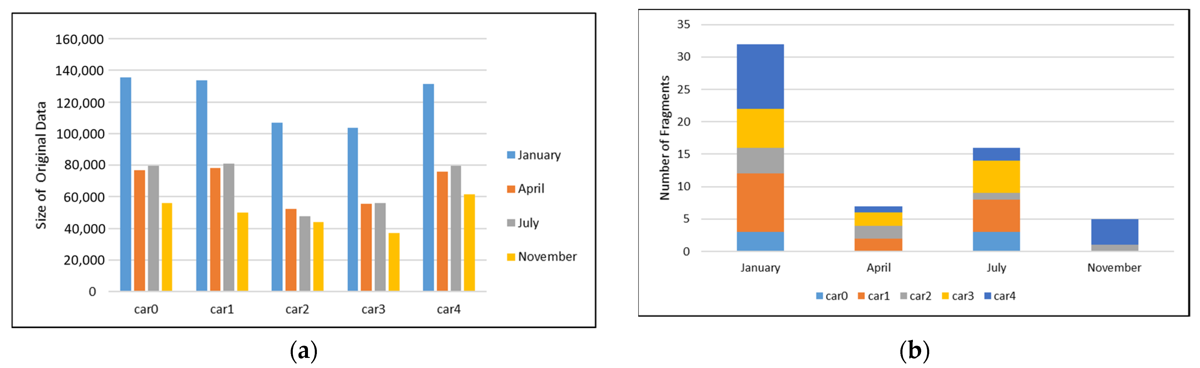
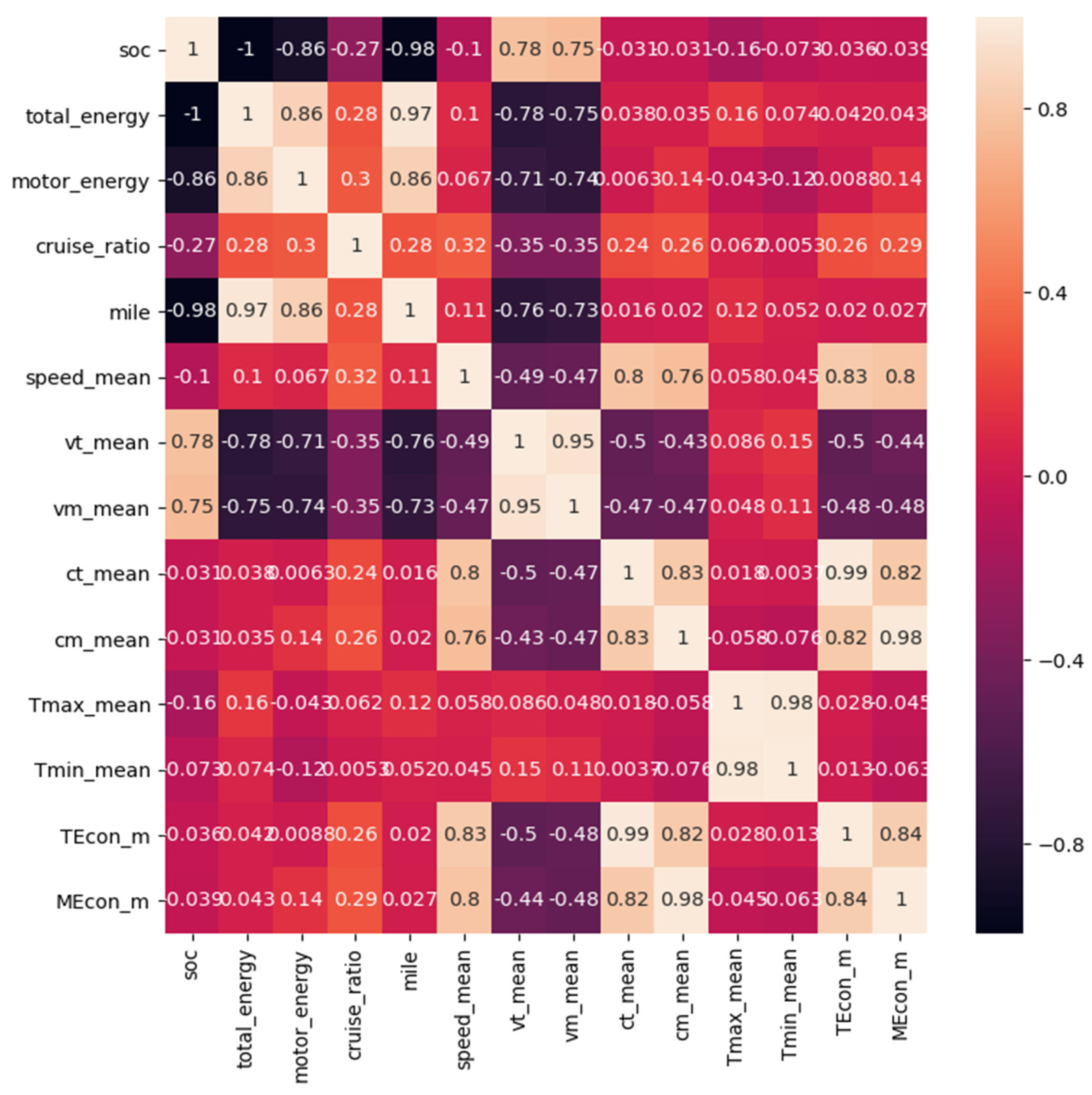
2.1. Analysis and Processing of Vehicle Driving Data

In this study, data were extracted from five vehicles (car0, car1, car2, car3, and car4) that were of the same model and size [17]. The data represented the actual on-road driving conditions within the period of a year; however, only four months (January, April, July, and November) were available for investigation. The total mileage traveled of each vehicle was between 30,000 and 80,000 km. The driving data of each electric vehicle contained both the charging process and discharging process, with 10Hz sampling data collection frequencies. Each set of data contained nine parameters to illustrate the vehicle performances over time, as listed in

Table 1. Nine measured parameters from each set of data.

Name	Sign	Unit	Notes
Time	t	s	Real-time data timestamp
Speed	speed	km/h	Real-time vehicle speed
Total voltage	vt	V	Total voltage
Total current	ct	A	Total current
Temp max	Tmax	°C	Maximum cell temperature
Temp min	Tmin	°C	Minimum cell temperature
Motor voltage	vm	V	Motor controller input voltage
Motor current	cm	A	Motor controller DC bus current
Mileage	Mile	km	Total mileage
SOC	SOC	%	State of charge

. The total number of collected data sets or sizes are shown in Figure 1a.

The data sets are fragmented in accordance to the vehicle’s SOC, in the range of 100% to 25%, and grouped into the respective month. This exercise was to ensure consistency in the prediction process and to evaluate accurately the strengths and weaknesses of the prediction methodology. Figure 1b depicts a total of 60 driving fragments distributed in accordance to the vehicles and months.

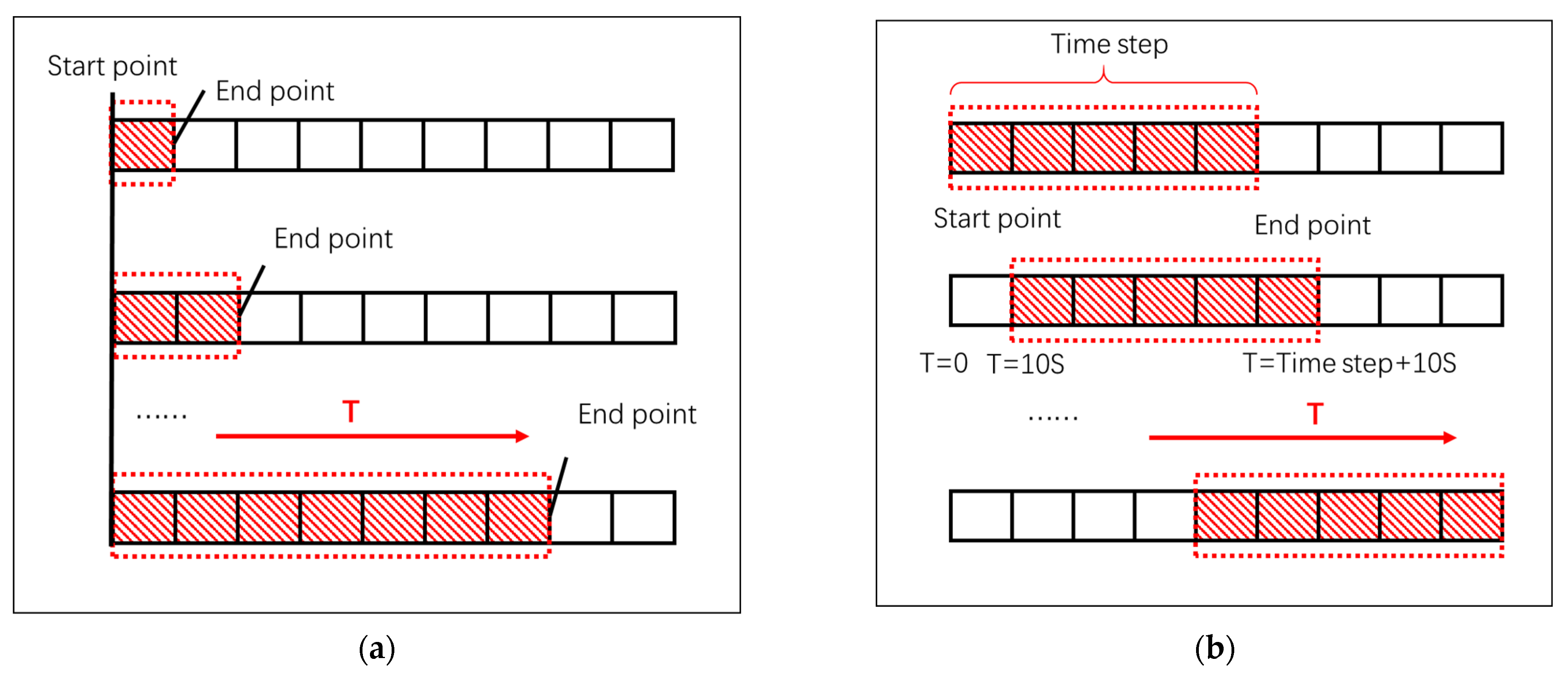
2.2. Sliding Window Method

The original data sets collected have nevertheless suffered from various data corruption problems, such as inconsistency, loss of data and segments, invalid ranges, abnormal patterns, etc. Data preprocessing is therefore crucial prior to any analysis or adoption to ensure that every data set adopted is healthy and consequential. The corrupted data were removed, and subsequently, the corresponding part was fitted by linear interpolation.

To analyze the original features of the data, the Pearson correlation coefficient was employed. By definition, the Pearson correlation coefficient measures the linear correlation between two certain features [18,19]. It is defined as the covariance of two variables, divided by the product of their standard deviations. Hence, the value is essentially the normalized measurement of the covariance, such that the result always has a value between −1 and 1. The formula is defined as follows:

$$\mathrm{r}=\frac{{{\displaystyle \sum }}_{i=1}^n\left(x_i-\overline{x}\right)\left(y_i-\overline{y}\right)}{\sqrt{{{\displaystyle \sum }}_{i=1}^n{\left(x_i-\overline{x}\right)}^2{{\displaystyle \sum }}_{i=1}^n{\left(y_i-\overline{y}\right)}^2}}$$

(1)

where r is the correlation coefficient, x_i is the values of the x-variable in a sample, $\overline{x}$ is the mean of the values of the x-variable, y_i is the values of the y-variable in a sample, $\overline{y}$ is the mean of the values of the y-variable.

Figure 2 demonstrates the weak correlation between the original features and the predicted target SOC. There are only two features “total voltage” and “motor voltage” that have relatively high correlation with SOC as compared to others; the values are, on average, 0.65 and 0.61 respectively. To further increase the correlation factors, we proposed the sliding time window (SW) method to extend the original features.

Generally, the SW method consists of a fixed-point sliding window and a dynamic sliding window. The fixed-point SW is a variable length interval sampling method with a fixed starting point and a sliding ending point along time. The illustrative principle is shown in Figure 3a. On the other hand, the dynamic SW is a sampling method that uses fixed-length temporal windows that shift to create instances. Each window position produces a fixed segment that is used to isolate data for later processing [20,21]. Figure 3b illustrates the principle.

By using the fixed-point sliding window method, the following extended features are created:

• Total energy consumption index (TE_con):

The total energy consumption measurement index of the whole vehicle battery module is defined as follows:

$$T{E}_{con}={{\displaystyle \int }}_0^t{v}_t\ast c_t dt$$

(2)

where t is the length of time window at the current time; v_t is the total voltage; c_t is the total current.

• Motor energy consumption index (ME_con):

The motor energy consumption measurement index of the motor module is calculated as follows:

$$M{E}_{con}={{\displaystyle \int }}_0^t{v}_m\ast c_m dt$$

(3)

where v_m is the motor voltage; c_m is the motor current.

The total energy consumption index ($T{E}_{con}$) and the motor energy consumption index ($M{E}_{con}$) are both time vectors. They are represented by the integral Equations (2) and (3), which show the content integral of two multiple parameters—the voltage and current. The current in this expression has both magnitude and direction, and, hence, is a vector quantity. The negative current indicates the vehicle in the regenerative or charging mode while the positive current indicates the discharging mode.

• Mileage driven (mile):

Driving distance of the vehicle in the current time window is defined as follows:

$$mile=mil{e}_t-mil{e}_0$$

(4)

• Cruise ratio (C_r):

The proportion of driving segment length in the current time window is used to measure the driving efficiency of the segments, which is defined as follows:

$$C_r=\frac{Count\left(m_c!=0\right)}{Len\left(T_{step}\right)}$$

(5)

where $Len\left(T_{step}\right)$ is the length of time window at the current time; m_c is the motor voltage.

In addition to the above, the dynamic SW allows us to obtain the mean values of some features as extended features, such as the mean values of speed ($spee{d}_m$) and total voltage ($v_{t\_m}$) in the dynamic time window. The overall extended features are summarized in

Table 2. Summary of the extended features descriptors.

Name	Sign	Unit	Notes
Total energy	TEcon	kw	Total energy consumption
Motor energy	MEcon	kw	Motor energy consumption
Mileage driven	mile	km/h	Mileage in the Fixed-point SW
Cruise ratio	Cr	%	The proportion of driving segment
Speed mean	speedm	km/h	The mean of speed in Dynamic SW
Total voltage mean	vt_m	V	The mean of vt in Dynamic SW
Motor voltage mean	vm_n	V	The mean of vm in Dynamic SW
Total current mean	ct_m	A	The mean of ct in Dynamic SW
Motor current mean	cm_m	A	The mean of cm in Dynamic SW
Temp max mean	Tmax_m	°C	The mean of Tmax in Dynamic SW
Temp min mean	Tmin_m	°C	The mean of Tmin in Dynamic SW
Total energy mean	TEcon_m	kw	The mean of TEcon in Dynamic SW
Motor energy mean	MEcon_m	kw	The mean of MEcon in Dynamic SW

.

The original data have a large degree of dispersion and asynchronous (with time delay) during data collections. By applying fixed-point and dynamic SW methods, the whole duration of the collected data can be captured and observed, and the average or cumulative values are extracted as new features, which significantly decrease the effects of the large instantaneous data dispersion and asynchronous data collection.

Figure 4 outlines the correlation of original features and extended features. After employing the SW method, the extended features have higher correlation with SOC than the original features. As illustrated, the features obtained by the fixed-point SW method have higher correlation as compared to Figure 2, with the maximum correlation value reaching 0.98. Furthermore, the dynamic SW method improves the correlation of the features “voltage” and “speed” to 0.1 and 0.78, respectively, which previously were only 0.063 and 0.65.

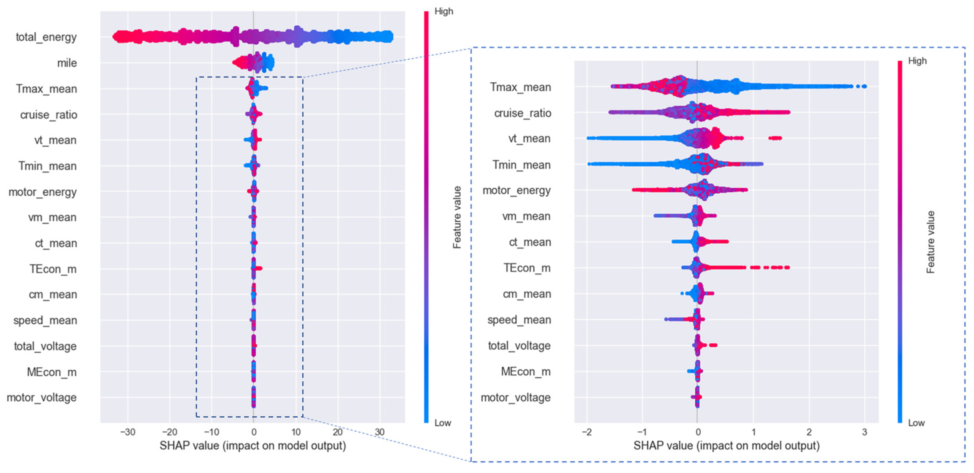
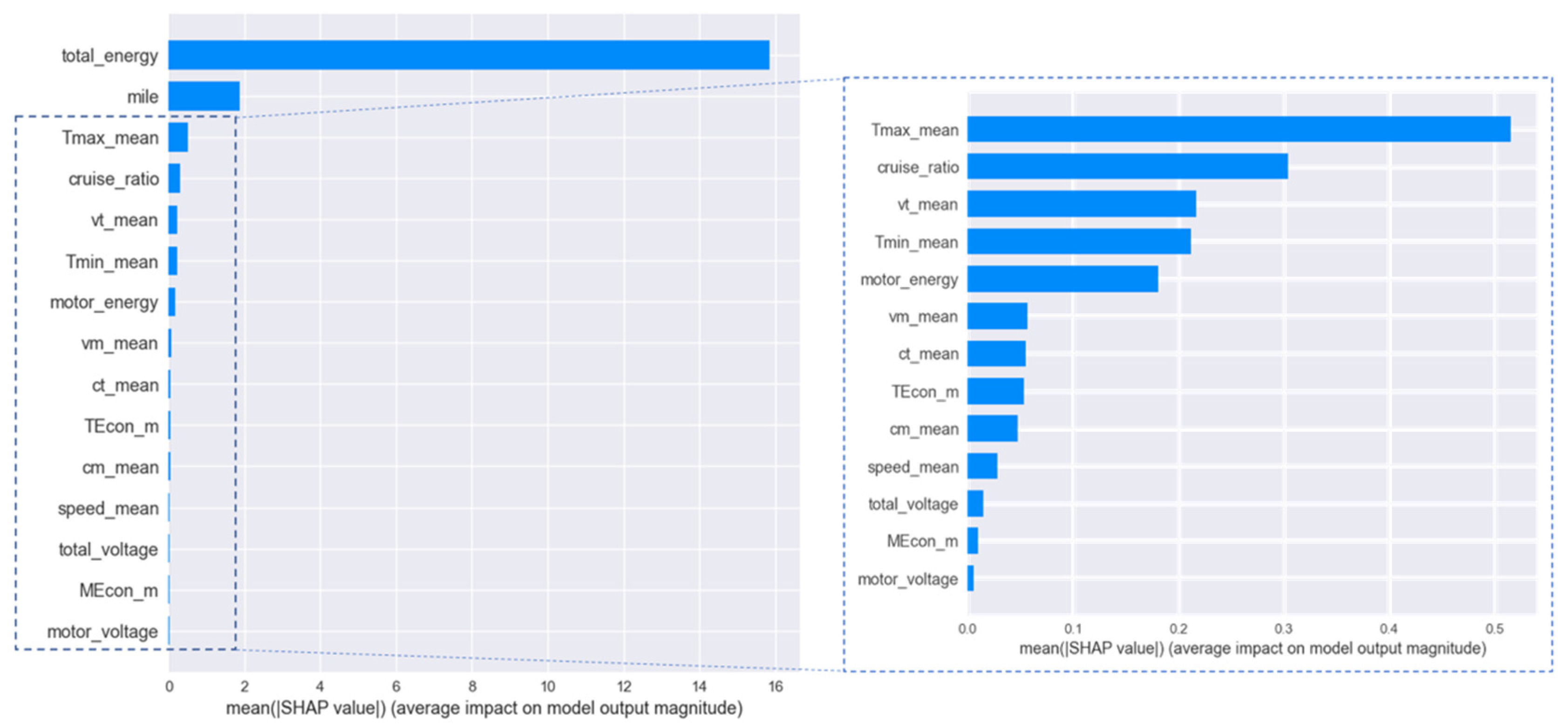
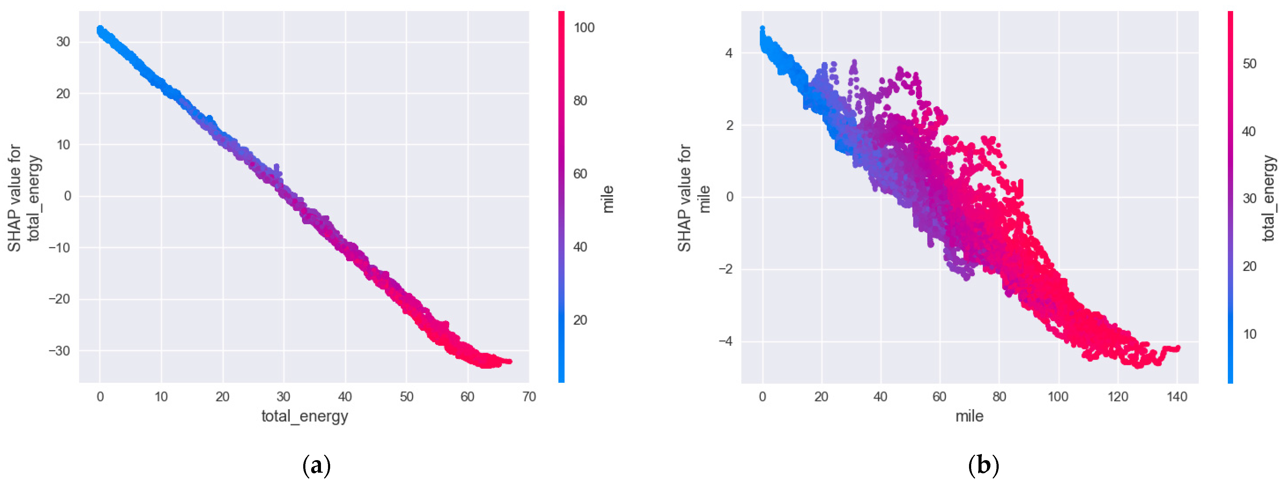
2.3. Machine Learning Algorithms and SHAP

In this section, three common traditional machine-learning algorithms were employed to learn the mapping relationship between the highly correlated features obtained in the previous section and the prediction target SOC. The three machine learning models are K-nearest neighbor algorithm (KNN), random forest (RFR) algorithm, and light gradient boosting machine algorithm (LightGBM).

The KNN algorithm can also effectively be used for regression problems [22]. KNN regression is used to predict the value of the output variable by using a local average, while KNN classification attempts to predict the class for the output variable through computing the local probability. In writing the algorithm for KNN, the regression technique only required an additional step to calculate the average value of data points as compared to the classifier. In this study, we used the KNeighborsRegressor from the machine learning scikit-learn library and its default parameters to train the model.

To evaluate the performances and perform comparison studies, three common statistical indicators were used: the coefficient of determination (R² score), mean absolute errors (MAE), and root mean square error (RMSE).

$$R^2=1-\frac{{{\displaystyle \sum }}_{i=1}^n{\left({\tilde{y}}_i-y_i\right)}^2}{{{\displaystyle \sum }}_{i=1}^n{\left(\overline{y}-y_i\right)}^2}$$

(6)

$$\mathrm{MAE}=\frac{1}{n}{\displaystyle \sum }_{i=1}^n\left|{\tilde{y}}_i-y_i\right|$$

(7)

$$\mathrm{RMSE}=\sqrt{\frac{1}{n}{\displaystyle \sum }_{i=1}^n{\left({\tilde{y}}_i-y_i\right)}^2}$$

(8)

where $y_1$,$y_2$,$\dots y_n$ are the actual values and ${\tilde{y}}_1$,${\tilde{y}}_2$,$\dots {\tilde{y}}_n$ are the predicted values, and $\overline{y}$ is the mean of $y_i$.

Here, the min–max normalization method is used to eliminate the influence of numerical differences on the prediction performance of regression models. Then, original features and extended features are applied to these machine-learning models, respectively. The results from the models are outlined in Figure 5, using both the original features (Figure 5a) and extended features (Figure 5b) as the input to the model. The comparison studies of the three models through the statistical indicators are listed in

Table 3. Performance of three machine-learning models on the dataset.

Algorithm	With Original Features			With Extended Features
	R2	RMSE	MAE	R2	RMSE	MAE
KNN	0.8127	9.0131	6.3559	0.9821	2.7796	2.0889
RF	0.8752	7.3579	5.2676	0.9923	1.8162	1.3087
LightGBM	0.8806	7.1984	5.5724	0.9941	1.5953	1.1640

.

The accuracy of the machine-learning model based on extended features is significantly improved with both the RMSE and MAE indicators reduced to at least three-fold. Further investigation also found that LightGBM algorithm has the best learning performance [23]. The LightGBM model used in this study has strong fitting capabilities due to its complex structure [24]. However, it is often regarded as a black-box model due to its large number of parameters, complex working mechanisms, and low transparency of the model.

The Shapley additive explanation (SHAP) method was used to improve the interpretability of the SOC prediction model and demonstrate the prediction of an instance x by computing the contribution of each feature to the prediction [25,26]. The SHAP value represents the contribution of each feature to the variation in the model output.

Based on the LightGBM model trained above, the impact of each feature is analyzed on the model output from a global perspective. In Figure 6, the blue indicator represents the value of the SHAP in direct proportion to the positive feedback to the output value, the same goes for the red indicator representing the negative feedback to the output value. Two features that have relatively strong correlation to the output model are “total energy” and “mile” followed by feature “Temp max mean”, as illustrated in the inset of Figure 6.

Through the SHAP explanatory analysis of the machine-learning model, we obtained the ranking of the influence degree of each feature on the output results of the model shown in Figure 7. Seven top ranked features of the SHAP value: “total energy”, “mile”, “temp max mean”, “cruise ratio”, “total voltage mean”, “temp min mean” and “motor energy mean” have apparently demonstrated more advantages over other features, which were used as the input to the LSTM model to learn time series features and predict SOC. Moreover, the two features “total energy” and “mile”, which had strong correlation with SOC, were further analyzed through the SHAP value and distributed, as portrayed in Figure 8. The two features show the inverse linear relationship with SOC, represented by the correlation value of SHAP. The dispersion in the vertical direction of a single feature can help reveal the degree of interaction with other features.

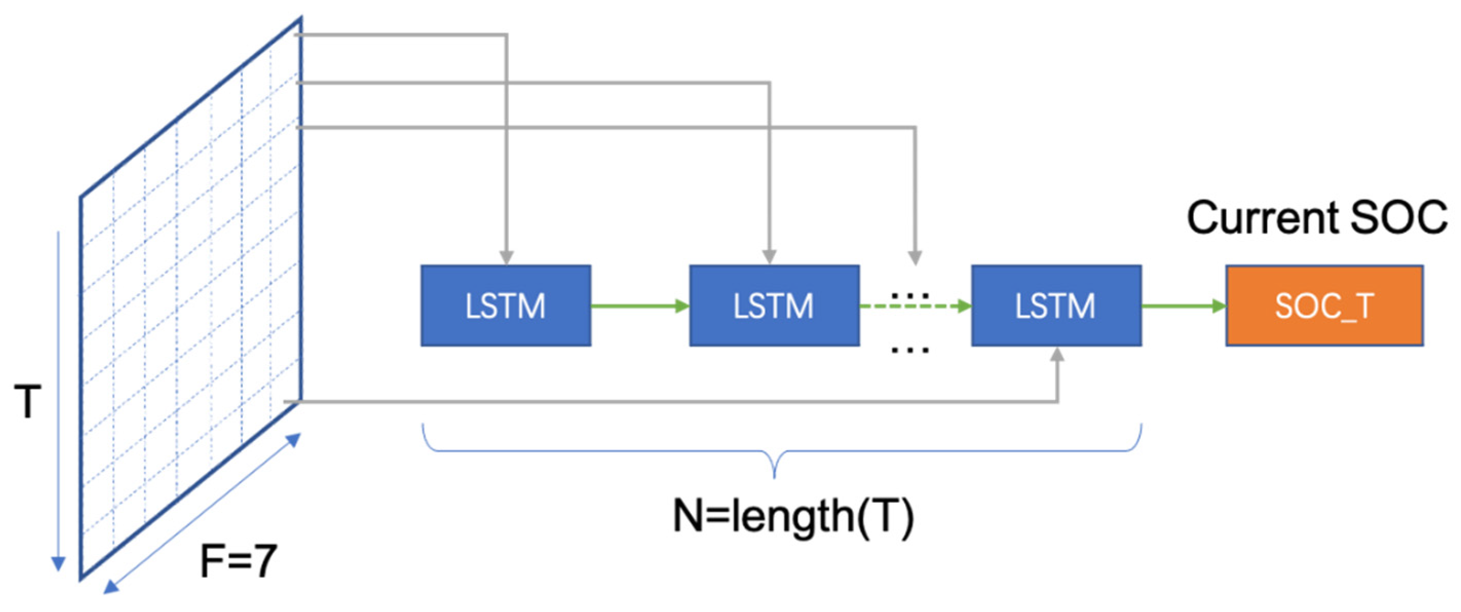
2.4. SOC Prediction with LSTM Model

In this section, we used the LSTM algorithm to predict SOC. The inputs to the LSTM model were the extended features processed by the SW and SHAP methods as described in previous sections. The long short-term memory network (LSTM) algorithm, which is an improved recurrent neural network (RNN) algorithm, is capable of learning long-term dependencies.

RNN is a kind of neural network used to process sequence data. The goal of neural network is to make neural network have memory functions, so that the current features can absorb the features from the remaining state, to improve the prediction accuracy of time series problems [27,28,29]. All RNNs have the form of a chain of repeating neural network modules. In standard RNNs, repeating modules have a simple structure, such as a single tanh layer. LSTM also contains a chain, but the repeating module has a different structure to interact, instead of having a single neural network layer [30,31,32,33].

The LSTM unit consists of three gates (input gate i, forgetting gate f, and output gate o), and several state memories: update step g, unit memory state C, and hidden state H. Input i is used to input the data of the current time step of the sequence and update the cell state. It adds the hidden state H of the previous cell and the current input X to the sigmoid function. The formula of the input gate is as follows:

$$i_t=\sigma \left(w_{xi}{x}_t+b_{xi}+W_{h_i}{h}_{t-1}+b_{h_i}\right)$$

(9)

where h_t−1 is the output of the hidden state of the last neuron; $\sigma$ is the activation function of sigmoid; w_xi is the input hidden layer weight matrix; W_hi is the hidden layer weight matrix; x_t is the input of the current neuron; b_hi is the bias that needs to be updated in the process of training; (annotation of the following formulas are similar.)

Forget gate f is used to determine the level of importance of that particular information and made decision on whether to discard of utilize the information. The input of this step is also the hidden state H of the previous unit, and the current input X. When you add them, and pass them to the sigmoid function, the formula for this step is as follows:

$$f_t=\sigma \left(w_{xf}{x}_t+b_{xf}+W_{h_f}{h}_{t-1}+b_{h_f}\right)$$

(10)

Update the process of cell memory state vector C:

$$g_t=\tanh (w_{xg}{x}_t+b_{xg}+W_{h_g}{h}_{t-1}+b_{h_g})$$

(11)

$$c_t=f_t\odot c_{t-1 }+i_t\odot g_{t }$$

(12)

where, c_t is the state vector of cell memory at time t; $\odot$ is Hadamard product.

Output gate o and hidden state H:

$$o_t=\sigma \left(w_{xo}{x}_t+b_{xo}+W_{h_o}{h}_{t-1}+b_{h_o}\right)$$

(13)

$$h_t=o_t\odot \tan \mathrm{h}\left(c_{t-1}\right)$$

(14)

The schematic diagram of LSTM network chain structure is shown in Figure 9.

The input of our LSTM model is the value of seven extended features in the latest previous time step. The time step is consistent with the length of the dynamic sliding time window, and the output is the current SOC. The proposed LSTM model is a chain structure with multiple inputs and a single output, as shown in Figure 10.

All data are input data for the LSTM model, in the unit of the time step. At each time step, seven features are input data for the LSTM model, at the same time, and then output for the predicted SOC after it is processed.

3. Results

In order to verify the accuracy and stability of the proposed SW-SHAP-LSTM method for SOC prediction, we distributed the training and test set accordingly. Approximately 90% of the fragments of each vehicle were randomly selected as the training set, and the remaining fragments were used as the test set.

Table 4. Randomly selected test set.

Vehicle	Test Set Frag Id	Month of Test Set	Total Number of Fragments
car0	4	July	6
car1	8, 9	January	16
car2	0	January	8
car3	6	April	13
car4	7, 10	November/January	17

provides the results of the random data set split.

Initial comparison was made between the original and extended features on the LSTM model to evaluate the respective performances. The plot in Figure 11 shows the prediction results of the fourth fragment of car0. The green plot represents the original features while the red one represents the extended features. As illustrated, the prediction though the extended features, after incorporating SW and SHAP methods—the accuracy is significantly improved. This is depicted in the overlapping curve between the red and blue curve.

The prediction accuracy of different models with extended features by the SW and SHAP methods were performed and evaluated with the proposed LSTM in this paper. The models generally selected for comparison are the widely used random forest regression (RFR) algorithm, light gradient boosting machine (LightGBM), and the K-nearest neighbor (KNN) algorithm. The results of the test sets are listed in

Table 5. Accuracy comparison of each model on the test set.

Model	RMSE	MAE	R2 Score (%)
KNN	2.749	2.065	98.26
RFR	1.829	1.315	99.25
LightGBM	1.631	1.180	99.39
Proposed LSTM	1.245	0.757	99.63

, with different statistical indicators, as detailed in Section 2. The proposed LSTM model returned the lowest value, which denoted higher accuracy as compared to the other three models. The notation R² in Table 5 is the coefficient of determination that is used to evaluate the performance of the linear regression model. The calculated value is directly proportional to the accuracy of the model prediction as analytically shown in Equation (6). In similar comparison studies, Figure 12 plots the percentage error resulted from each model prediction algorithm through the comparison with the actual measured SOC. The proposed LSTM model has the maximum error of 2.835%, which is the lowest among all the models employed for comparison.

Apart from the prediction accuracy studies of the proposed model, the stability or reliability of the model is also critical in ensuring repeatability and adaptability. Hence, the model is further verified through different driving fragments of different vehicles and different durations in the case months. The previously split training set data were employed, consisting of car1, car3, and car4 for the training and test groups, set from different months, as seen in Table 4. The results of the SOC prediction accuracy of fragments from different sources and durations are listed in

Table 6. Comparison of accuracy of different vehicles or seasonal test sets.

Segment	Month	Source	MSE	MAE	R2 Score (%)
car1 F8	January	Homologous	0.954	0.711	99.79
car3 F6	April	Homologous	1.072	0.707	99.64
car4 F7	November	Homologous	0.873	0.534	99.84
car0 F4	July	Heterogeneous	1.232	0.963	99.68
car2 F0	January	Heterogeneous	1.349	0.769	99.55
Car3 F6	April	Heterogeneous	1.003	0.873	99.57

. The notation ‘car i Fj’ represents the ’j’ th fragment of the ‘i’ th of the car. The column under the ‘Source’ is the data source of the test segment with ‘Homologous’, and denotes the test segment from the same vehicle, and ‘Heterogeneous’ from different vehicles.

4. Conclusions and Discussion

The SW-SHAP-LSTM method was proposed to predict the SOC of electric vehicles. The following are the investigation’s outcomes:

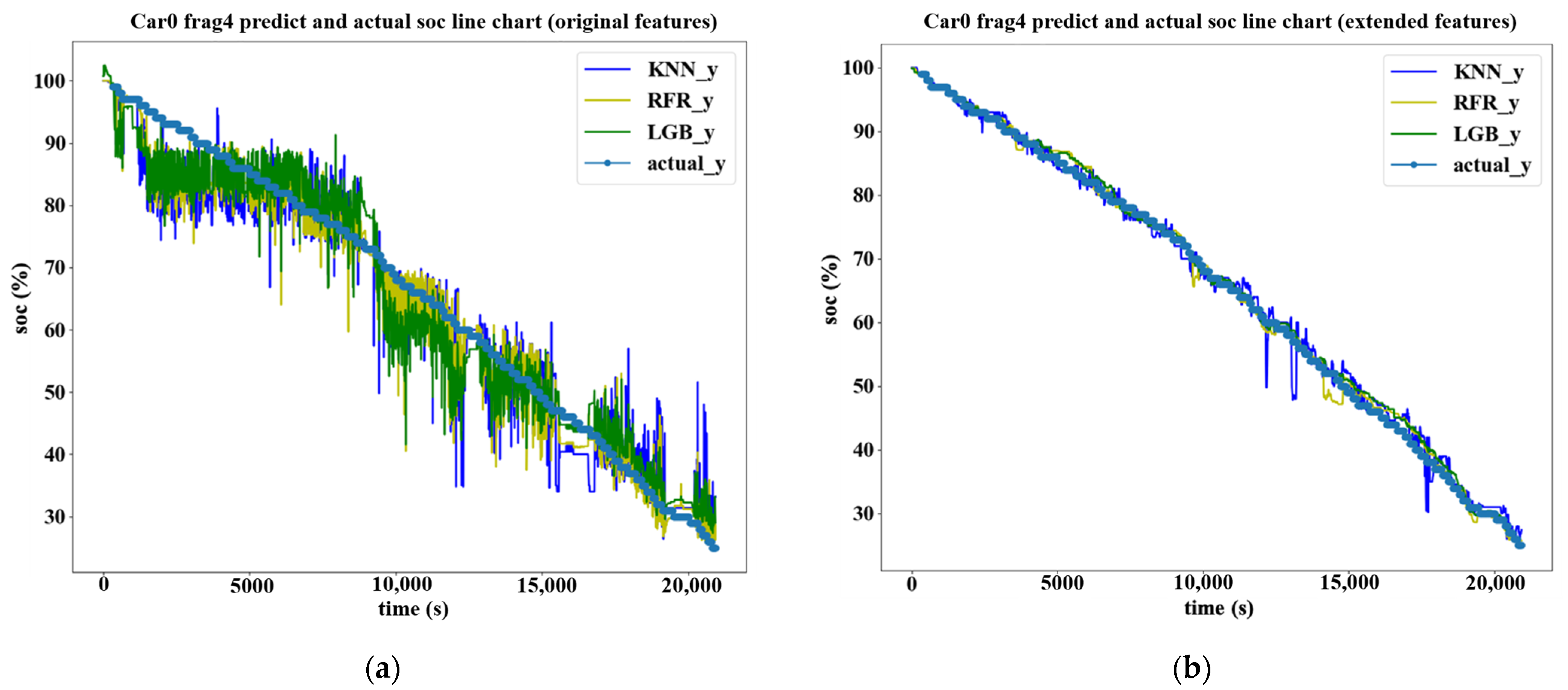
• Data preprocessing is crucial and necessary for machine learning. Data segregation and filtering will significantly improve the accuracy of models. The results from this investigation have shown that the extended features processed by the SW and SHAP methods can significantly reduce the prediction error and, hence, improve the accuracy.
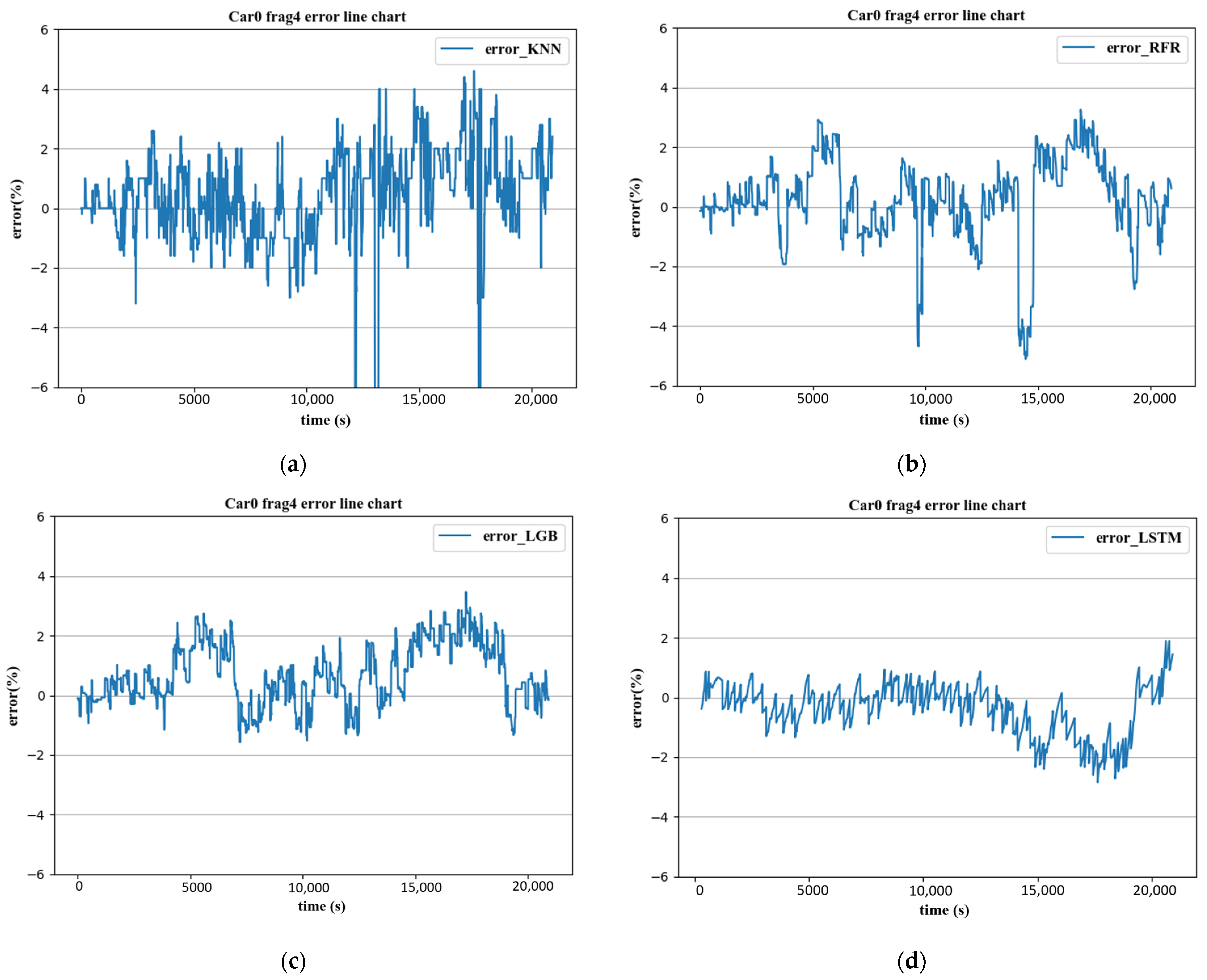
• LSTM has considerable advantages over other prediction models. The computed errors are within 2%, which is much lower than RFR, KNN, and LightGBM.
• The method proposed is shown to have good stability and adaptability, evidenced by the computed error on the prediction results when tested on the different vehicles and driving seasons.

Nevertheless, there is room to improve this study’s investigation. For instance, the range of SOC fragments can increase to more than 80%, as compared to the 75% in this study. Moreover, the machine learning models deployed in this study could further improve through the optimization techniques in the algorithm. This is because the LSTM method is susceptible to overfitting, high memory consumption during training, and is sensitive to different random weight initializations. The improved algorithm will focus on these shortcomings and incorporate the extended features with a filtering algorithm to estimate the initial SOC. Improving the distribution of training data set is also crucial for prediction accuracy. The distribution method used in this article was random distribution, but many methods are emerging, such as cross-validation, which can combine measures of fitness in prediction to derive a more accurate estimate of model prediction performance.

References

1. Sun, F.; Hu, X.; Zou, Y.; Li, S. Adaptive unscented Kalman filtering for state of charge estimation of a lithium-ion battery for electric vehicles. Energy 2011, 36, 3531–3540. [Google Scholar] [CrossRef]
2. Ardeshiri, R.R.; Balagopal, B.; Alsabbagh, A.; Ma, C.; Chow, M.-Y. Machine Learning Approaches in Battery Management Systems: State of the Art: Remaining useful life and fault detection. In Proceedings of the 2020 2nd IEEE International Conference on Industrial Electronics for Sustainable Energy Systems (IESES), Cagliari, Italy, 20–22 April 2020; pp. 61–66. [Google Scholar]
3. Rauh, N.; Franke, T.; Krems, J.F. Understanding the impact of electric vehicle driving experience on range anxiety. Hum. Factors 2015, 57, 177–187. [Google Scholar] [CrossRef]
4. Zhu, Y.; Gao, T.; Fan, X.; Han, F.; Wang, C. Electrochemical techniques for intercalation electrode materials in rechargeable batteries. Acc. Chem. Res. 2017, 50, 1022–1031. [Google Scholar] [CrossRef]
5. Wang, Y.; Tian, J.; Sun, Z.; Wang, L.; Xu, R.; Li, M.; Chen, Z. A comprehensive review of battery modeling and state estimation approaches for advanced battery management systems. Renew. Sustain. Energy Rev. 2020, 131, 110015. [Google Scholar] [CrossRef]
6. Hannan, M.A.; Lipu, M.H.; Hussain, A.; Mohamed, A. A review of lithium-ion battery state of charge estimation and management system in electric vehicle applications: Challenges and recommendations. Renew. Sustain. Energy Rev. 2017, 78, 834–854. [Google Scholar] [CrossRef]
7. Chandran, V.; Patil, C.K.; Karthick, A.; Ganeshaperumal, D.; Rahim, R.; Ghosh, A. State of charge estimation of lithium-ion battery for electric vehicles using machine learning algorithms. World Electr. Veh. J. 2021, 12, 38. [Google Scholar] [CrossRef]
8. Liu, K.; Li, K.; Peng, Q.; Zhang, C. A brief review on key technologies in the battery management system of electric vehicles. Front. Mech. Eng. 2019, 14, 47–64. [Google Scholar] [CrossRef] [Green Version]
9. Xiong, R.; Cao, J.; Yu, Q.; He, H.; Sun, F. Critical review on the battery state of charge estimation methods for electric vehicles. IEEE Access 2017, 6, 1832–1843. [Google Scholar] [CrossRef]
10. Hu, J.; Hu, J.; Lin, H.; Li, X.; Jiang, C.; Qiu, X.; Li, W. State-of-charge estimation for battery management system using optimized support vector machine for regression. J. Power Sources 2014, 269, 682–693. [Google Scholar] [CrossRef]
11. Jiao, M.; Wang, D.; Qiu, J. A GRU-RNN based momentum optimized algorithm for SOC estimation. J. Power Sources 2020, 459, 228051. [Google Scholar] [CrossRef]
12. Hasan, A.J.; Yusuf, J.; Faruque, R.B. Performance comparison of machine learning methods with distinct features to estimate battery SOC. In Proceedings of the 2019 IEEE Green Energy and Smart Systems Conference (IGESSC), Long Beach, CA, USA, 4–5 November 2019; pp. 1–5. [Google Scholar]
13. Hannan, M.A.; Lipu, M.H.; Hussain, A.; Ker, P.J.; Mahlia, T.; Mansor, M.; Ayob, A.; Saad, M.H.; Dong, Z. Toward enhanced State of charge estimation of Lithium-ion Batteries Using optimized Machine Learning techniques. Sci. Rep. 2020, 10, 1–15. [Google Scholar] [CrossRef] [Green Version]
14. Hong, J.; Wang, Z.; Chen, W.; Wang, L.-Y.; Qu, C. Online joint-prediction of multi-forward-step battery SOC using LSTM neural networks and multiple linear regression for real-world electric vehicles. J. Energy Storage 2020, 30, 101459. [Google Scholar] [CrossRef]
15. Song, X.; Yang, F.; Wang, D.; Tsui, K.-L. Combined CNN-LSTM network for state-of-charge estimation of lithium-ion batteries. IEEE Access 2019, 7, 88894–88902. [Google Scholar] [CrossRef]
16. Houlian, W.; Gongbo, Z. State of charge prediction of supercapacitors via combination of Kalman filtering and backpropagation neural network. IET Electr. Power Appl. 2018, 12, 588–594. [Google Scholar] [CrossRef]
17. Technology, Beijing Institute of Technology. Prediction of SOC in the Driving Process of Electric Vehicles. Available online: http://www.ncbdc.top (accessed on 15 November 2020).
18. Benesty, J.; Chen, J.; Huang, Y.; Cohen, I. Pearson correlation coefficient. In Noise Reduction in Speech Processing; Springer: Berlin, Germany, 2009; pp. 1–4. [Google Scholar]
19. Benesty, J.; Chen, J.; Huang, Y. On the importance of the Pearson correlation coefficient in noise reduction. IEEE Trans. Audio Speech Lang. Process. 2008, 16, 757–765. [Google Scholar] [CrossRef]
20. Smrithy, G.; Balakrishnan, R.; Sivakumar, N. Anomaly detection using dynamic sliding window in wireless body area networks. In Data Science and Big Data Analytics; Springer: Berlin, Germany, 2019; pp. 99–108. [Google Scholar]
21. Laguna, J.O.; Olaya, A.G.; Borrajo, D. A dynamic sliding window approach for activity recognition. In Proceedings of the International Conference on User Modeling, Adaptation, and Personalization, Girona, Spain, 11–15 July 2011; pp. 219–230. [Google Scholar]
22. Hu, C.; Jain, G.; Zhang, P.; Schmidt, C.; Gomadam, P.; Gorka, T. Data-driven method based on particle swarm optimization and k-nearest neighbor regression for estimating capacity of lithiumion battery. Appl. Energy 2014, 129, 49–55. [Google Scholar] [CrossRef]
23. Islam, M.K.; Hridi, P.; Hossain, M.S.; Narman, H.S. Network anomaly detection using lightgbm: A gradient boosting classifier. In Proceedings of the 2020 30th International Telecommunication Networks and Applications Conference (ITNAC), Melbourne, Australia, 25–27 November 2020; pp. 1–7. [Google Scholar]
24. Sun, X.; Liu, M.; Sima, Z. A novel cryptocurrency price trend forecasting model based on LightGBM. Financ. Res. Lett. 2020, 32, 101084. [Google Scholar] [CrossRef]
25. Lundberg, S.; Lee, S.-I. A unified approach to interpreting model predictions. arXiv 2017, arXiv:1705.07874. [Google Scholar]
26. Tan, S.; Caruana, R.; Hooker, G.; Koch, P.; Gordo, A. Learning global additive explanations for neural nets using model distillation. arXiv 2018, arXiv:1801.08640. [Google Scholar]
27. Yang, F.; Li, W.; Li, C.; Miao, Q. State-of-charge estimation of lithium-ion batteries based on gated recurrent neural network. Energy 2019, 175, 66–75. [Google Scholar] [CrossRef]
28. Li, C.; Xiao, F.; Fan, Y. An approach to state of charge estimation of lithium-ion batteries based on recurrent neural networks with gated recurrent unit. Energies 2019, 12, 1592. [Google Scholar] [CrossRef] [Green Version]
29. Zhao, R.; Kollmeyer, P.J.; Lorenz, R.D.; Jahns, T.M. A compact unified methodology via a recurrent neural network for accurate modeling of lithium-ion battery voltage and state-of-charge. In Proceedings of the 2017 IEEE Energy Conversion Congress and Exposition (ECCE), Cincinnati, OH, USA, 1–5 October 2017; pp. 5234–5241. [Google Scholar]
30. Hochreiter, S.; Schmidhuber, J. Long short-term memory. Neural Comput. 1997, 9, 1735–1780. [Google Scholar] [CrossRef]
31. Graves, A. Long short-term memory. In Supervised Sequence Labelling with Recurrent Neural Networks; Springer: Berlin, Germany, 2012; pp. 37–45. [Google Scholar]
32. Yang, F.; Song, X.; Xu, F.; Tsui, K.-L. State-of-charge estimation of lithium-ion batteries via long short-term memory network. IEEE Access 2019, 7, 53792–53799. [Google Scholar] [CrossRef]
33. Zhao, Z.; Chen, W.; Wu, X.; Chen, P.C.; Liu, J. LSTM network: A deep learning approach for short-term traffic forecast. IET Intell. Transp. Syst. 2017, 11, 68–75. [Google Scholar] [CrossRef] [Green Version]
Figure 1. Original data size and number of fragments. (a) Distribution of the original data from different vehicles and different months; (b) fragmentation in according to SOC range from 100% to 25%, and distributed accordingly to vehicles and months.
Energies 14 03692 g001
Figure 2. The correlation of the original features.
Energies 14 03692 g002
Figure 3. Schematic diagram of sliding time window sampling. (a) Fixed-point sliding window method; (b) dynamic sliding window method.
Energies 14 03692 g003
Figure 4. Extended feature correlation graph.
Energies 14 03692 g004
Figure 5. Comparison chart of machine learning model results. (a) Original features are used as input; (b) extended features are used as input.
Energies 14 03692 g005
Figure 6. Global interpretation of output SOC by SHAP value of other extended features.
Energies 14 03692 g006
Figure 7. Mean value ranking of SHAP values characteristic.
Energies 14 03692 g007
Figure 8. SHAP value distribution and interaction of two important features. (a) SHAP value distribution of “total energy” feature; (b) SHAP value distribution of “mile” feature.
Energies 14 03692 g008
Figure 9. LSTM network chain structure.
Energies 14 03692 g009
Figure 10. Our LSTM chain structure.
Energies 14 03692 g010
Figure 11. Comparison of original features and extended features by SW-SHAP.
Energies 14 03692 g011
Figure 12. Error comparison of each model. (a) The error of the KNN prediction model; (b) the error of the RFR prediction model; (c) the error of the LightGBM prediction model; (d) the error of the proposed LSTM prediction model.
Energies 14 03692 g012