Abstract
Fault interpretation is an important part of seismic structural interpretation and reservoir characterization. In the conventional approach, faults are detected as reflection discontinuity or abruption and are manually tracked in post-stack seismic data, which is time-consuming. In order to improve efficiency, a variety of automatic fault detection methods have been proposed, among which widespread attention has been given to deep learning-based methods. However, deep learning techniques require a large amount of marked seismic samples as a training dataset. Although the amount of synthetic seismic data can be guaranteed and the labels are accurate, the difference between synthetic data and real data still exists. To overcome this drawback, we apply a transfer learning strategy to improve the performance of automatic fault detection by deep learning methods. We first pre-train a deep neural network with synthetic seismic data. Then we retrain the network with real seismic samples. We use a random sample consensus (RANSAC) method to obtain real seismic samples and generate corresponding labels automatically. Three real 3D examples are included to demonstrate that the fault detection accuracy of the pre-trained network models can be greatly improved by retraining the network with a few amount of real seismic samples.
1. Introduction
Interpreting faults from seismic data plays an important role in the subsurface structural interpretation and reservoir evaluation since faults can behave as a seal or a conduit for oil and gas transportation, and fault fracture zones are also favorable spaces for hydrocarbon accumulation in carbonate rock areas [1]. In conventional fault interpretation, interpreters identify the faults as reflection discontinuity or abruption and track faults on 2D or 3D seismic images, which is very operator-intensive, and deeply relies on the experience of interpreters. In order to assist fault interpretation, a set of seismic attributes which highlight the reflection discontinuities have been proposed. One of the famous attributes is coherence [2,3], which highlights faults by measuring similarity between seismic traces. Another type of attribute highlights faults by computing the difference between seismic traces, e.g., variance attribute [4], curvature attribute [5] and gradient magnitude [6]. Since these attributes are with seismic reflection removed and discontinuities highlighted, they can be regarded as fault images.
Recently, with the development of machine learning algorithms, a set of convolutional neural network-based methods have been introduced to assist in seismic fault interpretation. Araya-Polo et al. [7] propose to train a deep neural network that directly detects the faults from the raw seismic data. Huang et al. [8] use a synthetic seismic volume and a suit of corresponding attributes to train the faults identification network. Some authors suggest detecting faults by pixel-wise classification with seismic attributes using CNN methods [9,10]. Xiong et al. extract training samples from field seismic data and train a fault classification CNN network [11]. Di et al. apply the multi-layer perceptron technique to detect faults on multiple seismic attribute patches [12]. Wu et al. train a CNN model based on synthetic seismic patches, the trained model can not only detect faults but also estimate the fault orientation [13]. To improve efficiency, Wu et al. use U-net to train an end-to-end 3D fault detection network [14]. Wu et al. propose a multitask learning scheme to simultaneously solve fault detection, edge-preserving smoothing and normal estimation by using a single U-net architecture [15]. Besides fault detection, deep learning techniques have also been widely applied in many other fields of seismic data processing and interpretation, e.g., noise attenuation [16,17], 3D reservoir modeling [18] and seismic data interpolation and reconstruction [19,20]. Recently, transfer learning has also attracted the attention of many researchers [21,22].
Although deep learning methods have made encouraging progress in automatic fault detection, there are still some drawbacks that restrict the application of these methods in real data. A large amount of seismic data with accurate labels is required for the supervised learning methods. Synthetic seismic data can meet the requirement of quantity and label accuracy, but cannot meet the requirement of actual geological diversity. Cunha et al. use synthetic seismic data to obtain a pre-trained CNN model, and apply the transfer learning strategy by retraining the model on the real seismic samples which are selected and labelled from real seismic data manually [23]. However, obtaining real training samples by manually picking still depends on the experience of interpreters. In this paper, we propose a transfer learning strategy to improve the performance of seismic fault detection by using CNN. We firstly generate synthetic seismic patches with accurate labels, then train the CNN model with these synthetic samples. Using the real data as training samples, we follow the fine-tuning strategy to train the entire network with initial weights equal to the pre-trained model weights. Three 3D seismic examples demonstrate that our method can effectively improve fault detection accuracy.
In this research, we propose an automatic method to obtain real seismic samples and corresponding labels. To obtain the real seismic data patches and corresponding labels, we calculate the fault enhancement attribute for a sub-volume of the real seismic data, in this work, the fault enhancement attribute is calculated by applying a forward and backward filter on coherence cube. With the fault enhancement attribute, we randomly choose the seismic patches and calculate the labels by using a random sample consensus (RANSAC) algorithm. The workflow of the proposed methods is shown in Figure 1b. We also demonstrate the Schematic diagram of fault surface modelling in Figure 1a.
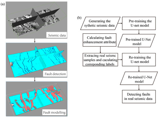
Figure 1.
Schematic diagram of fault surface modelling (a) and block diagram of proposed methods (b).
2. Methods
2.1. CNNs and Pre-Trained Model
Training a CNN model often requires a large number of samples and corresponding labels. Manually picking the faults on the real seismic data is time-consuming and highly subjective. Compared with obtaining training samples from real seismic data, there are several advantages to creating training samples from synthetic seismic images. First of all, the synthetic seismic data have sufficient quantity and diversity, in other words, the number of training samples, the features of faults, the SNR of seismic image and the dominant frequency of wavelet, all of these can be artificially specified and adjusted. In addition, the synthetic data are with accurate labels, which is more beneficial to the training and optimization of the network. We follow the method of Wu et al. [13] to generate the synthetic seismic data. A horizontal reflectivity model with a reflectivity sequence randomly selected within [−1, 1] is first created. Then, a sine function and a linear shearing function with random parameters are applied to the reflectivity model to simulate the folding and faulting. The synthetic seismic images can be obtained by convolving the reflectivity model with a Ricker wavelet of the random dominant frequency. Random noise is also added to these seismic data in order to increase the authenticity of synthetic data. The dip angles are defined in the range of [−86, −65] and [65, 86]. We generate 32,000 synthetic fault patches and 18,000 non-fault patches for training, we also generate 5000 synthetic seismic images for validating. Figure 2 shows part of the training images and their corresponding labels. The patch size of the training image is 48 × 32 pixels.
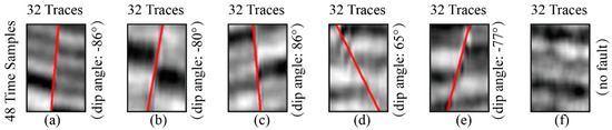
Figure 2.
Some synthetic training samples, red solid lines indicate their corresponding labels.
A convolutional neural network is a class of deep neural network, most commonly applied to image processing such as classification, segmentation, object detection [24] and so on. Detecting fault in seismic data can be regarded as either an image classification problem or image segmentation problem. U-net was firstly developed for biomedical image segmentation [25], and then it was widely applied to many other image segmentation. In this work, we choose U-net to train the model of fault detection.
The U-net architecture in this studyis shown in Figure 3. The output layer is a 1 × 1 convolutional layer with a sigmoid activation function to output the fault probability map which has the same size as the input image. To solve the problem of an unbalanced distribution of zero and one pixels (most pixels are labeled by zero), we use the following balanced cross-entropy loss function [26],
where n is the number of pixels in the input seismic patch. denotes the true label and represents the prediction probability for ith pixel. represents the ratio of non-fault pixels in the seismic patch. The Adam algorithm [27] is adopted to optimize the loss function. The learning rate is 0.0001, and the batch size is 256. After training the network with 20 epochs, the training and validation accuracies increase to 0.98, and the training and validation loss converges to 0.01. A 2D seismic section is selected to test the fault detection effect of the pre-trained network, the fault detection result is shown in Figure 4. The pre-trained network can detect part of faults correctly, however, there are still many faults that have not been detected, and there are also some misidentifications, which are indicated by white and black arrows in Figure 4.
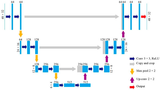
Figure 3.
The U-net architecture for fault detection.
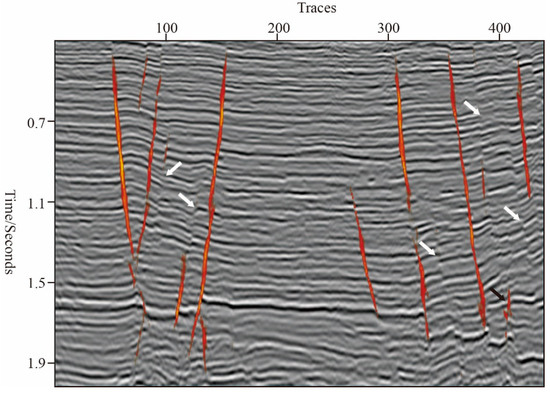
Figure 4.
A 2D seismic section is displayed with the fault probability predicted by the pre-trained U-net model.
2.2. Real Seismic Patches for Transfer Learning
Although the diversity of synthetic data can be guaranteed by randomly setting the parameters such as dominant frequency and SNR, the dissimilarity between synthetic data and real seismic data still exists. It can be seen from Figure 4 that the pre-trained network models are with high recognition accuracy on the synthetic validation data, but the fault detection results on the real seismic image are not satisfactory. In order to improve the effectiveness of the network in detecting the faults on real seismic images, we adopt a transfer learning strategy that retrains the pre-trained network with a small amount of real seismic patches.
Manually picking and labeling the seismic patches on real seismic data is a way to generate training samples for transfer learning, however, this method is cumbersome, and the accuracy of labeling depends on the experience of the interpreter. To overcome these drawbacks, we adopt a scheme to automatically choose and label the seismic patches from real seismic data.
- Step 1: Calculating fault enhancement attribute
Since the fault is not the main feature in the seismic images and is manifested as reflection discontinuities or interruptions, many fault attributes are proposed to highlight fault. However, the fault attributes may be noisy because these attributes are also sensitive to some non-fault structures such as channels and strata pinch-out. To show the faults more directly, many fault enhancement attributes have been proposed. Some authors suggest improving the fault continuity and suppress non-fault features by using swarm intelligence [28,29]. Machado et al. [30] proposed a fault enhancement technology by using a directional Laplacian of Gaussian (LoG) filter. In this paper, we use a forward and backward diffusion method [31] to generate the fault enhancement attributes (Figure 5b).
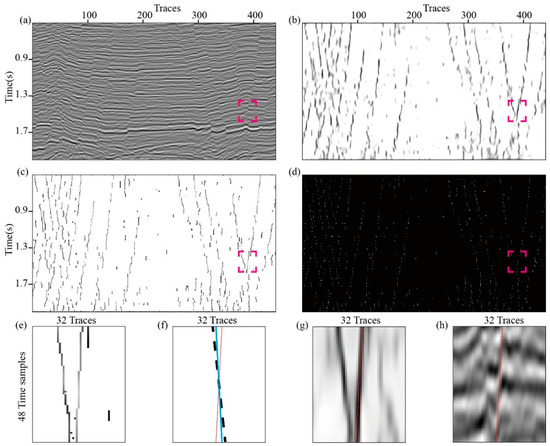
Figure 5.
The workflow of generating real fault samples and corresponding labels. We first calculate the fault enhancement attribute (b) on the seismic images (a). We then apply non-maximum suppression on the fault enhancement attribute to obtain the thinned fault image (c) and get the seed points (d). Centered on the seed points, the windowed thinned fault images (e) are extracted. The fault orientations are estimated based on the windowed thinned fault images and the labels can be obtained (f). The fault label is overlaid with the fault enhancement attribute (g) and seismic image (h).
- Step 2: generating fault and non-fault samples
With the fault enhancement attributes, our next step is to automatically obtain the seed points and extract the fault patches at each seed point. We first apply non-maximum suppression to the original fault enhancement attribute to generate a thinned fault attribute (Figure 5c). In this thinned fault attribute, only the attribute values on the ridges can be preserved and the attribute values on other places are set to zero. Then, a threshold and a radius are defined, points with attribute values less than the specified threshold are selected as candidate points, in which only the two adjacent candidate points with a distance greater than the specified radius can be identified as true seed points. (Figure 5d). Thirdly, a local thinned fault image is extracted, and the window size is 48 × 32. Finally, the dip angle of the fault is estimated and the label of the fault sample can be obtained. The fault orientation can be estimated by the structure–tensor-based method ([2]), PCA-based methods [32] and scanning-based method [33]. However, these methods are not suitable for estimating fault orientation in thinned fault attribute, because most of the attribute values are zero and multi-oriented intersecting faults occur. In this paper, we use a RANSAC algorithm to estimate fault orientations [34]. With this method, the seed point is a required point, and other points are randomly selected to calculate the best fitting parameters of the fault plane. The effectiveness and accuracy of using the RANSAC algorithm to calculate fault orientations and then generate fault sample labels can be demonstrated in the bottom row of Figure 5. Figure 5e shows a small patch of thinned fault image which is indicated by the red dashed rectangle in Figure 5c. There are two faults with close distance and opposite dipping direction in this small patch, which will lead to estimation errors of fault direction by using PCA-based method (black dashed line in Figure 5f) or structure–tensor-based method (blue solid line in Figure 5f). The red solid line in Figure 5f indicates the fault direction estimated by the RANSAC algorithm. We also overlaid the estimation fault direction with fault enhancement attribute (Figure 5g) and seismic image (Figure 5h) to verify the accuracy of the fault direction. The corresponding label can be easily obtained by setting ones on a red solid line and zeros elsewhere.
We also need to automatically obtain the seed points and pick the non-fault patches at each seed point for transfer learning. Different from the generation process of fault samples, the seed points of non-fault samples are directly located in the fault enhancement attribute rather than in the thinned fault attribute. Then, by defining a threshold and a radius, points with attribute values greater than the specified threshold and the minimum distance between two adjacent points greater than the specified radius are selected as seed points. Finally, taking seed points as the center, the seismic image patches are extracted as non-fault samples and corresponding labels are with the same size patches in which values are all equal to zero.
By using this method, we can automatically construct the library which contains real fault and non-fault samples for transfer learning. Figure 6 shows some samples and corresponding labels extracted from the real dataset. For this 3D seismic data (751 [vertical] × 440 [crossline] × 201 [inline] samples), we build a library with more than 10,000 fault samples and more than 20,000 non-fault samples. However, not all the samples are involved in transfer learning. We randomly choose 1000 fault samples and 2000 non-fault samples to retrain the pre-trained CNN model. We also randomly pick up 1000 samples for validation. In the retraining process, the learning rate is 5 × 10e−5, the batch size is 128, and we retrain the network with 10 epochs. After retraining the pre-trained network with real samples, the validation accuracy on real validation sets is increased from 73% to 96%.
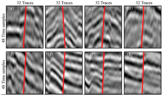
Figure 6.
Examples of real samples and corresponding labels.
3. Results
The first 3D seismic volume used to test the effect of transfer learning is the seismic data we use to extract the real training samples. Figure 7a shows the fault probability predicted by using the pre-trained U-Net model. Since the pre-trained model only uses synthetic data as training samples, it is difficult to guarantee the similarity to the real seismic data. As a result, many faults have not been detected. After using real seismic samples for transfer learning, the model can identify most faults accurately, the fault probability predicted by the retrained model is shown in Figure 7b. In Figure 8, we select two inline sections and one-time slice to illustrate the impact of transfer learning on the accuracy of fault detection. The left column and right column in Figure 8 are the fault probability predicted by the U-Net model before and after transfer learning respectively. The pre-trained U-Net model can detect some faults with sharp reflection discontinuities and strong amplitude, however, many faults that are not so obvious have not been detected. After transfer learning, the accuracy and continuity of the faults were greatly improved.
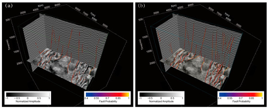
Figure 7.
The first 3D seismic data are displayed with faults probabilities that are predicted by using (a) the pre-trained U-Net model and (b) the U-Net model after transfer learning.
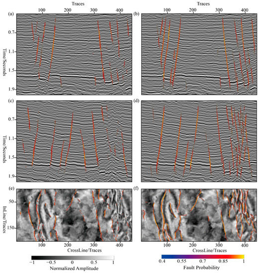
Figure 8.
Faults detection results on the first 3D seismic data by using the pre-trained U-Net model (left column) and the U-Net model after transfer learning (right column), and all results are overlaid on corresponding seismic image. Vertical slices and horizontal slice are inline 50 (a,b), inline 150 (c,d) and time = 1500 ms (e,f), respectively.
It might not be surprising that the U-Net model after transfer learning can improve the accuracy of fault detection in the first 3D seismic data because the real training samples for transfer learning are also extracted from the first 3D seismic volume. To verify the robustness of the network model after transfer learning, we further apply the same U-Net model on the other two field seismic data which are acquired at different surveys.
The second 3D seismic data in Figure 9 are a subset (501 [vertical] × 441 [inline] × 441 [crossline]) of the seismic data which are acquired in Eastern China. The fault detection results by using a pre-trained U-Net model are shown in Figure 9a. Figure 9b shows the fault probability predicted by the U-Net model after transfer learning. We also choose one inline section and one-time slice to compare the fault detection results by using the U-Net model before (Figure 10a,c) and after (Figure 10b,d) transfer learning. Similar to the first example, the pre-trained U-Net model fails to detect many faults, while the network model after transfer learning accurately identifies most faults.
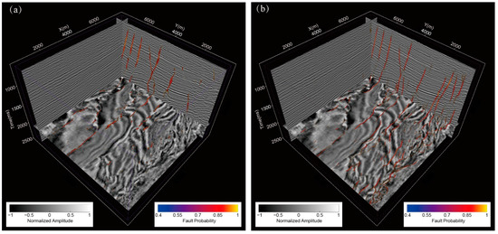
Figure 9.
The second 3D seismic data are displayed with faults probabilities that are predicted by using (a) the pre-trained U-Net model and (b) the U-Net model after transfer learning.
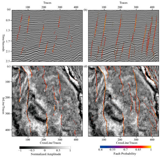
Figure 10.
Comparison of the faults detection results on 2D slices by using the pre-trained U-Net model (left column) and the U-Net model after transfer learning (right column). Vertical slice and horizontal slice are inline 360 (a,b) and time = 1600 ms (c,d), respectively.
The third 3D seismic data in Figure 11 are a subset (401 [vertical] × 191 [inline] × 700 [crossline]) of Kerry-3D which is provided on the SEG Wiki website. The fault detection results by using a pre-trained U-Net model are shown in Figure 11a. Figure 11b shows the fault probability predicted by the U-Net model after transfer learning. We also choose one inline section and one-time slice to compare the fault detection results by using the U-Net model before (Figure 12a,c) and after (Figure 12b,d) transfer learning. As shown in Figure 12a, the faults with small vertical displacement (indicated by white arrows) cannot be detected, the reason might be that the synthetic training samples are not comprehensive enough, however, after transfer learning with a small amount of real seismic samples, these faults can be accurately identified.
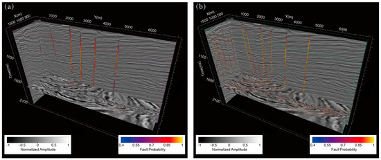
Figure 11.
A subset of Kerry-3D seismic data is displayed with faults probabilities that are predicted by using (a) the pre-trained U-Net model and (b) the U-Net model after transfer learning.
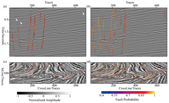
Figure 12.
Comparison of the faults detection results on 2D slices by using the pre-trained U-Net model (left column) and the U-Net model after transfer learning (right column). Vertical slice and horizontal slice are inline 50 (a,b) and time = 1200 ms (c,d), respectively.
In summary, only using 3000 real seismic samples in transfer learning significantly improves the fault detection accuracy of the pre-trained network models that are trained with synthetic samples. Moreover, the real seismic samples for transfer learning are all extracted from the first 3D seismic data, and the retrained network models can also work pretty well in the second and third seismic data, indicating that the retrained network models can be used for detecting similar type of faults in a different area.
4. Discussion
Generally speaking, compared with traditional fault detection methods (e.g., ant tracking method), the CNN-based method has significant advantages. First, it is very efficient. The traditional method needs to calculate the fault image from seismic data, and then use the fault enhancement algorithm to perform the fault detection. The CNN-based method is to detect faults directly based on seismic data; secondly, the fault detection effect does not depend on the parameter settings. Traditional methods rely heavily on parameters, and it is necessary to adjust the parameters multiple times to achieve the best detection effect. Of course, the CNN-based method also has disadvantages, that is, it is highly dependent on the training dataset. A network model trained solely with synthetic samples is hard to achieve satisfactory results on real seismic data, and extraction of real seismic samples and manually labeling faults are very cumbersome and time-consuming. In this paper, by combining the forward and backward diffusion method and RANSAC method, we proposed a scheme to automatically extract real samples from fault enhancement attributes and generate corresponding labels. The real samples are used to retrain the U-net model which is pre-trained based on the synthetic samples. U-Net is an end-to-end network used for semantic segmentation. It uses relatively large size training samples and windows for fault detection in seismic data. The main advantage is high efficiency compared with classification networks using the sliding window method to detect faults. However, we still use small size training samples and the sliding window method for the following reason. We assume the fault in the small window can be seen as a plane, then we can use the proposed method to calculate the fault orientations. Based on this assumption, the labels of real seismic samples calculated in a smaller window will be more accurate. Although we use U-Net in a relatively “dumb” way, the computational cost is still acceptable. By using one RTX 2080ti GPU, it takes about 30 min to compute the fault probability of the second 3D seismic data. Although current examples are all implemented in 2D, extending the method to 3D is straightforward.
In our present research, although we adopted a method to extract real seismic samples and calculate labels automatically, our approach still belongs to the scope of supervised learning, the extraction of real samples and calculation of labels are still affected by parameters. In future research, we will treat synthetic seismic data as source domain data and real seismic data as target domain data, and then adopt an unsupervised domain adaption method to further reduce the dependence on parameter settings.
5. Conclusions
The effectiveness of fault detection using a deep learning framework greatly depends on the diversity of training samples and the accuracy of corresponding labels. The synthetic samples can guarantee the accuracy of the labels, but it is difficult to guarantee that it has the same features with the real seismic data. Obtaining real samples manually in the field seismic data is time-consuming and subjective, moreover, the accuracy of labels cannot be guaranteed. In this paper, we propose a method to automatically extract real samples and generate corresponding labels. Based on these real seismic samples, we retrain the entire network with initial weights equal to those of the pre-trained model which is trained with synthetic samples. We present three 3D seismic examples to illustrate that the retrained network models with a few amount real samples can greatly improve the performance of the pre-trained network models. Although all the real samples are obtained from the first 3D seismic data, the retrained models also work well on the other two seismic data, which shows the generalization of the retrained models.
However, we still focus on the faults that appear with reflection discontinuities, and avoid the more complex fault types such as thrust and listric faults. Since these faults show strong reflection features in seismic data, which are difficult to be highlighted by conventional fault attributes, they increase the difficulty to obtain real samples and corresponding labels accurately. We will focus on these issues in future research.
Author Contributions
Conceptualization, Z.Y. and Z.Z.; methodology, Z.Y.; coding, Z.Z.; designing the experiments, S.L. and Z.Z. All authors have read and agreed to the published version of the manuscript.
Funding
This research is supported by the National Natural Science Foundation of China under Grant No. 41974125.
Data Availability Statement
The Kerry 3D seismic data can be found at https://wiki.seg.org/wiki/Kerry-3D, accessed on 18 July 2020.
Acknowledgments
The authors wish to thank the editors and three anonymou s reviewers for their comments that greatly improved the manuscript.
Conflicts of Interest
The authors declare no conflict of interest.
References
- Lu, X.; Wang, Y.; Yang, D.; Wang, X. Characterization of paleo-karst reservoir and faulted karst reservoir in Tahe Oilfield, Tarim Basin, China. Adv. Geo-Energy Res. 2020, 4, 339–348. [Google Scholar] [CrossRef]
- Bahorich, M.S.; Farmer, S.L. 3D seismic discontinuity for faults and stratigraphic features. Lead. Edge 1995, 14, 1053–1058. [Google Scholar] [CrossRef]
- Wu, X. Directional structure-tensor based coherence to detect seismic faults and channels. Geophysics 2017, 82, A13–A17. [Google Scholar] [CrossRef]
- Van Bemmel, P.P.; Pepper, R.E. Seismic Signal Processing Method and Apparatus for Generating a Cube of Variance Values. U.S. Patent 6,151,555, 21 November 2000. [Google Scholar]
- Di, H.; Gao, D. Efficient volumetric extraction of most positive/negative curvature and flexure for fracture characterization from 3d seismic data. Geophys. Prospect. 2016, 64, 1454–1468. [Google Scholar] [CrossRef]
- Aqrawi, A.A.; Boe, T.H. Improved Fault Segmentation Using a Dip Guided and Modified 3D Sobel Filter; SEG Expanded Abstracts: San Antonio, TX, USA, 2011; pp. 999–1003. [Google Scholar]
- Araya-Polo, M.; Dahlke, T.; Frogner, C.; Zhang, C.; Poggio, T.; Hohl, D. Automated fault detection without seismic processing. Lead. Edge 2017, 36, 208–214. [Google Scholar] [CrossRef]
- Huang, L.; Dong, X.; Clee, T.E. A scalable deep learning platform for identifying geologic features from seismic attributes. Lead. Edge 2017, 36, 249–256. [Google Scholar] [CrossRef]
- Guitton, A. 3D convolutional neural networks for fault interpretation. In Proceedings of the 80th Annual Conference and Exhibition, EAGE, Extended Abstracts, Copenhagen, Denmark, 11–14 June 2018; pp. 1–5. [Google Scholar]
- Guo, B.; Li, L.; Luo, Y. A New Method for Automatic Seismic Fault Detection Using Convolutional Neural Network; SEG Expanded Abstracts: Anaheim, CA, USA, 2018; pp. 1951–1955. [Google Scholar]
- Xiong, W.; Ji, X.; Ma, Y.; Wang, Y.; AlBinHassan, N.M.; Ali, M.N.; Luo, Y. Seismic fault detection with convolutional neural network. Geophysics 2018, 83, O97–O103. [Google Scholar] [CrossRef]
- Di, H.; Shafiq, M.; AlRegib, G. Patch-Level Mlp Classification for Improved Fault Detection; SEG Expanded Abstracts: Anaheim, CA, USA, 2018; pp. 2211–2215. [Google Scholar]
- Wu, X.; Shi, Y.; Fomel, S.; Liang, L. Convolutional Neural Networks for Fault Interpretation in Seismic Images; SEG Expanded Abstracts: Anaheim, CA, USA, 2018; pp. 1946–1950. [Google Scholar]
- Wu, X.; Liang, L.; Shi, Y.; Fomel, S. FaultSeg3D: Using synthetic datasets to train an end-to-end convolutional neural network for 3D seismic fault segmentation. Geophysics 2019, 84, IM35–IM45. [Google Scholar] [CrossRef]
- Wu, X.; Liang, L.; Shi, Y.; Geng, Z.; Fomel, S. Multitask learning for local seismic image processing: Fault detection, structure-oriented smoothing with edge-preserving, and seismic normal estimation by using a single convolutional neural network. Geophys. J. Int. 2019, 219, 2097–2109. [Google Scholar] [CrossRef]
- Saad, O.M.; Chen, Y. Deep denoising autoencoder for seismic random noise attenuation. Geophysics 2020, 85, V367–V376. [Google Scholar] [CrossRef]
- Li, S.; Yang, X.; Liu, H.; Cai, Y.; Peng, Z. Seismic data denoising based on sparse and low-rank regularization. Energies 2020, 13, 372. [Google Scholar] [CrossRef]
- Yao, J.; Liu, Q.; Liu, W.; Liu, Y.; Chen, X.; Pan, M. 3D Reservoir Geological Modeling Algorithm Based on a Deep Feedforward Neural Network: A Case Study of the Delta Reservoir of Upper Urho Formation in the X Area of Karamay, Xinjiang, China. Energies 2020, 13, 6699. [Google Scholar] [CrossRef]
- Pan, S.; Yan, K.; Lan, H.; Badal, J.; Qin, Z. A sparse spike deconvolution algorithm based on a recurrent neural network and the iterative shrinkage-thresholding algorithm. Energies 2020, 13, 3074. [Google Scholar] [CrossRef]
- Chai, X.; Tang, G.; Wang, S.; Lin, K.; Peng, R. Deep Learning for Irregularly and Regularly Missing 3-D Data Reconstruction. IEEE Trans. Geosci. Remote Sens. 2020. [Google Scholar] [CrossRef]
- El Zini, J.; Rizk, Y.; Awad, M. A deep transfer learning framework for seismic data analysis: A case study on bright spot detection. IEEE Trans. Geosci. Remote Sens. 2019, 58, 3202–3212. [Google Scholar] [CrossRef]
- Wu, B.; Meng, D.; Wang, L.; Liu, N.; Wang, Y. Seismic impedance inversion using fully convolutional residual network and transfer learning. IEEE Geosci. Remote Sens. Lett. 2020, 17, 2140–2144. [Google Scholar] [CrossRef]
- Cunha, A.; Pochet, A.; Lopes, H.; Gattass, M. Seismic fault detection in real data using transfer learning from a convolutional neural network pre-trained with synthetic seismic data. Comput. Geosci. 2020, 135, 104344. [Google Scholar] [CrossRef]
- Zhao, Z.Q.; Zheng, P.; Xu, S.T.; Wu, X. Object detection with deep learning: A review. IEEE Trans. Neural Netw. Learn. Syst. 2019, 30, 3212–3232. [Google Scholar] [CrossRef] [PubMed]
- Ronneberger, O.; Fischer, P.; Brox, T. U-net: Convolutional networks for biomedical image segmentation. In Proceedings of the International Conference on Medical Image Computing and Computer-Assisted Intervention, Munich, Germany, 5–9 October 2015; pp. 234–241. [Google Scholar]
- Xie, S.; Tu, Z. Holistically-nested edge detection. In Proceedings of the IEEE International Conference on Computer Vision, Santiago, Chile, 7–13 December 2015; pp. 1395–1403. [Google Scholar]
- Kingma, D.P.; Ba, J. Adam: A method for stochastic optimization. arXiv 2014, arXiv:1412.6980. [Google Scholar]
- Pedersen, S.I.; Randen, T.; Sønneland, L.; Steen, O. Automatic Fault Extraction Using Artificial Ants; SEG Expanded Abstracts: Salt Lake City, UT, USA, 2002; pp. 512–515. [Google Scholar]
- Yan, Z.; Gu, H.; Cai, C. Automatic fault tracking based on ant colony algorithms. Comput. Geosci. 2013, 51, 269–281. [Google Scholar] [CrossRef]
- Machado, G.; Alali, A.; Hutchinson, B.; Olorunsola, O.; Marfurt, K.J. Display and enhancement of volumetric fault image. Interpretation 2016, 4, SB51–SB61. [Google Scholar] [CrossRef]
- Yan, Z.; Liu, S.; Gu, H. Fault image enhancement using a forward and backward diffusion method. Comput. Geosci. 2019, 131, 1–14. [Google Scholar] [CrossRef]
- Barnes, A.E. A filter to improve seismic discontinuity data for fault interpretation. Geophysics 2006, 71, P1–P4. [Google Scholar] [CrossRef]
- Wu, X.; Hale, D. 3D seismic image processing for faults. Geophysics 2016, 81, IM1–IM11. [Google Scholar] [CrossRef]
- Fischler, M.A.; Bolles, R.C. Random sample consensus: A paradigm for model fitting with applications to image analysis and automated cartography. Commun. ACM 1981, 24, 381–395. [Google Scholar] [CrossRef]
Publisher’s Note: MDPI stays neutral with regard to jurisdictional claims in published maps and institutional affiliations. |
© 2021 by the authors. Licensee MDPI, Basel, Switzerland. This article is an open access article distributed under the terms and conditions of the Creative Commons Attribution (CC BY) license (https://creativecommons.org/licenses/by/4.0/).