Abstract
In the interests of the environment, many countries set limits on the use of non-renewable energy sources and promote renewable energy sources through policy and legislation. Consequently, the demand for components for renewable energy systems exhibits an upward trend. For this reason, managers, investors, and banks are interested in knowing whether investing in a business associated with the semiconductor and related device manufacturing sector, especially the photovoltaic (PV) systems manufacturers, is worthy of a penny. Using a sample for the period of 2015–2018, we apply a new approach to panel data, extending existing research using Classification Trees with the k-Nearest Neighbor and Altman model. Our aim is to analyze the financial conditions of enterprises to identify key indicators that distinguish companies producing PV system components (labeled “green, G”) from companies that do not manufacture PV components (“red, R”). Our results show that green companies can be distinguished from red companies at classification accuracies of 86% and 90% for CRT and CHAID algorithms in Classification Trees method and 93% for k-Nearest Neighbor method, respectively. Based on the Altman model and the analysis of crucial ratios, we also find that green businesses are characterized by lower financial performance although future ratio values may equal or exceed the values for the red companies if current upward trends are sustained. Therefore, investing in green companies presents a viable alternative.
1. Introduction
Debates about renewable energy sources have become more prominent in recent decades with increased public acceptance and a positive perception of renewable energy source [1]. Given the negative effects of the increased consumption of fossil fuels which include climate change and global warming, policymakers and researchers have shown an increased focus on and preference for renewable energy sources. This increasing preference has resulted in the share of electricity generated from renewable sources exceeding 25% in 2018 and is consistent with an upward trend in the production of renewable energy over the three preceding decades [2]. Policy makers, aiming to reduce dependence on fossil fuels, which are unequally distributed across geographies and often can be found in volatile and conflict zones, have sought to promote the transition from fossil fuels to renewable energy sources by setting target levels for the production of electricity from renewable energy sources. For example, India and China have set targets of 40% and 50% of total energy production from renewable sources, respectively. Turkey is aiming to produce 30% of electricity from renewable energy sources by 2030, whereas Thailand has set a target of 26% by 2036. To date, only Turkey has achieved its target [2,3,4]. The setting of targets, rising reliance upon and growing preference for renewable energy sources means that investment in electricity from renewable energy sources must increase. This, in turn, implies increased demand for components used in the production of electricity from renewable sources; solar modules, solar cells, silicon rods, photovoltaic equipment, and equipment. Given these targets and preference for renewable energy sources, there has been much interest in renewable energy and related aspects.
For example, [5,6,7,8] discuss and outline policy measures implemented in the EU-27, the United States, Canada, Germany, and other top renewable energy producers to promote the development and investment in renewable energy production and the use of renewable energy. There is also a body of work that examines the impact of oil prices, carbon prices, and carbon-pass through rates on renewable energy stocks [9,10,11,12,13,14,15]. Other aspects considered are the relationship between corporate environmental performance and environmental performance [16,17,18,19], corporate social responsibility and competitiveness [20], environmental performance, [21,22], productivity and efficiency [23], financial distress and failure [24,25], and factors that impact firms’ decisions to engage in a proactive environmental strategy [16].
For investment to take place, firms associated with renewable energy production—whether directly or through the manufacturing of components used in the production of renewable energy—must present an attractive alternative for investors by exhibiting profitability or high potential future returns. A number of studies investigate the performance of firms associated with renewable energy production. Ruggiero and Lehkonen [17] investigate the relationship between the financial performance of electric utilities over the short and the long-term and an increase in the production of renewable energy. Their sample comprises 66 electric utilities in North America, the European Union, and East Asia over a period spanning 2005 to 2014. The return on assets (ROA), return on equity (ROE), and Tobin’s q (ratio of a firm’s market value to the book value of total assets) are used as measures of financial performance and renewable energy production is expressed in gigajoules. They report a negative relationship between increases in renewable energy production and both short and long-term financial performance, suggesting that the deployment of renewable energy may not necessarily have positive implications for electric utilities operating in mature markets owing to high capital costs. Halkos and Tzeremes [26] apply a data envelopment analysis to assess the performance of Greek firms operating within the renewable energy sector using a limited number of financial ratios. They find that financial performance is associated with lower levels of debt and high levels of return on assets. Firms that produce wind energy outperform firms that generate hydropower. Their study does not contrast the performance of firms within renewable energy sector—green companies—against red firms. Paun [27] contrasts the financial performance of Romanian firms that produce fossil fuels against those that are involved in the production of renewable energy using a sample of 91 energy producers over the period of 2012 to 2015. After analyzing financial ratios measuring profitability and returns on equity, they find that companies that produce fossil fuels perform better than those involved in the production of green energy. Paun [27] goes onto report that the performance of green companies deteriorates after 2013 and that RES firms have offered relatively low returns on equity. This is attributed to changes in government and delays in issuing green certificates resulting in low levels of investment in green firms. Ruggiero and Lehkonen [17] conclude that RES companies are close to financial distress. Notably, Paun [27] omits a number of key measures of financial performance due to limitations in the data, these being return on investment and the current ratio. Tomczak [28] investigates whether power utilities that produce electricity using renewable energy sources are more profitable than power utilities producing electricity using fossil fuels. Following a consideration of 16 ratios for 37 companies located in Baltic and Central European countries, Tomczak [28] finds that RES companies exhibit lower returns on assets and returns on equity relative to fossil fuel producers suggesting that RES companies are not as profitable as fossil fuel companies, which are shown to be more profitable. Rastogi et al. [29] report upon the trend of ROE for Renewable Energy companies (RES companies) in India and the United States. They argue that given the large investment required to develop renewable energy sources, the renewable energy sector needs to exhibit profitability or the potential for profitability in the future in order to attract investors. Using k-Means Cluster analysis and a sample comprising 14 Indian and 14 United States (US) renewable energy companies for the period of 2015–2019, they report somewhat mixed results. Indian companies operating in the wind and hybrid energy sector show declines in financial performance, whereas the companies involved in solar energy show improvements in ROE between 2016 and 2017. Most Indian companies exhibit either relatively constant ROE or unstable and declining ROE. In the United States, the ROE for predominantly solar energy companies declined between 2016 and 2017 and then increased marginally before either remaining constant or declining towards 2019. The US companies operating predominantly in the wind energy sector showed increasing ROEs between 2017 before the ROE began experiencing a decline towards 2019. For both Indian and the US RES companies, some fluctuations can be observed for the majority of companies between 2015 and 2019, with generally positive ROEs. However, a definitive or strong upward trend in the ROE for RES companies does not emerge. In other words, RES companies do not appear to offer increasing returns.
This study builds upon the previous work of Tomczak et al. [30] who set out to determine whether investing in so-called “green”—companies that are associated with the production of photovoltaic (PV) components used in the production of renewable energy sources–offers a greater return on investment relative to investing in “red” companies, the latter relating to companies that do not manufacture PV components. Tomczak et al. [30] considered over 2000 companies, mostly operating in China and applied classification tree analysis for classifying companies as “red” or “green” using the financial ratios. They also identified key ratios for classifying, having considered a total of 62 ratios for the year 2017. Their findings are somewhat unexpected and in the negative form. Investing in “green” companies does not appear to be lucrative and RES-related companies are not as financially sounder relative to companies in the general semiconductor and solid-state device manufacturing sector. The authors go onto recommend that investors should be cautious about investing in green companies with it remaining to be seen whether statutory determined targets will increase demand and whether this will translate into increasing profits.
Section 2 presents the data used in the study and the methodology applied. In this section, we provide an overview of the databases used and the sample size considered in our analysis. We list the ratios considered in the analysis (Table 1) and outline the algorithms applied for the purpose of classifying green and red companies on the basis of ratios. Section 3 set out the empirical results. Here, we summarize the results of the application of the algorithms. Results indicate that the Chi-squared Automatic Interaction Detector (CHAID), Classification and Regression Trees (CRT), and k-Nearest Neighbors algorithms perform relatively well in classifying green and red companies on the basis of ratios, in-sample, and out-of-sample. Of these, the best performing algorithm is the k-Nearest Neighbors algorithm, whereas the CRT algorithm underperforms both algorithms. Once we have identified ratios that can be used to distinguish between green and red companies, we apply the Altman model to assess financial performance. In Section 4, the results are discussed. We note that red companies outperform green companies. However, green companies show an improvement in key ratios over time. This suggests that in the near future, green companies may outperform red companies as a critical mass is established and investment in green companies continues to increase. Section 5 concludes the study.

Table 1.
List of ratios considered.
2. Data and Methodology
Our methodology comprised a number of steps. First, we collected data from financial reports for companies from the related device manufacturing sector. Financial statements were downloaded from the Emerging Markets Information Service (EMIS) database, a Euromoney Institutional Investor Company (www.emis.com, accessed on 23 June 2020). The initial sample consists of companies operating in Chinese Taipei (236 companies). To identify whether investing in businesses that manufacture RES components was profitable, we divided businesses in the sector into two groups. The first group comprised companies that manufacture solar modules, solar cells, solar silicon rods, solar wafers, solar power, solar photovoltaic products, and related equipment—“green” companies. The second group comprised businesses that are not associated with RES companies—“red” companies. The number of companies in our samples was unbalanced due to the unbalanced number of companies associated with RES sector. This means that the number of green companies was much lower relative to the number of red companies. There were 36 companies operating in Chinese Taipei in the green group, while 200 companies in the red group.
A panel data set was used in this study. We used the panel data set due to the following reasons. This increases the database that can be used for statistical analysis. It also permits the capturing of changes in indicators over time for firms in the sample. A panel dataset comprises data for the same observations over time [31]. Consequently, panel studies permit the analysis of general trends and provide objective information about the occurring phenomena. They make it possible to indicate the anticipated changes of the studied phenomenon and show regularities. It is therefore possible to determine which events have an impact on the studied phenomenon. Additionally, they make it possible to organize events over time. The basic limitation encountered in the course of conducting panel studies is, inter alia, the possibility of losing representativeness or increasing research costs [32]. Panel data are used in many fields of science [33,34,35].
The second step was to calculate the 92 ratios used in this study from the balance sheet and the profit and loss accounts, cash flow information, and market values for the businesses in our sample. Most of these ratios were considered in previous studies (62 ratios, whereas 30 are new). The ratios considered characterized different aspects of financial performance, namely, liquidity, profitability, turnover, debt, and market values (see Table 1). Such ratios have been widely used in the analysis of the financial standing of businesses for the purposes of bankruptcy prediction [36].
We used several methods of statistical analysis. Among others, these include Classification Trees and the k-Nearest Neighbors methods to classify enterprises into established “green” and “red” enterprises.
We applied Classification Trees for a number of reasons. Classification Trees are a family of statistical methods that use diagrams to sequentially divide the data space into categories classes with similar properties. They are easy to understand and interpret. They do not require data preparation. Other techniques often require data normalization, creating blind variables, or removing blank values. Trees can handle both numeric and categorical data. They are robust, efficient, and quick to work with large amounts of data.
The goal was to build a tree with a minimum number of nodes. Then, the criteria received were simpler and easy to interpret. The general form of the algorithm consists of the following steps:
- With a set of K objects, determine that they belong to the same class. If so, end the algorithm.
- Otherwise, consider all possible divisions of set K into subsets K1, K2,... Kn so that they are as homogeneous as possible.
- Assess these divisions according to the adopted criteria and select the best one.
- Divide set K in the chosen way.
- Perform steps 1–4 recursively for each subset.
The subject of division is an N-element set of objects. Here, these are enterprises that are described by M + 1 ratios (e.g., retained earnings/total assets, (gross profit + extraordinary items + financial expenses)/total assets). It follows that vector [x, y] with the ratios M can be stated as follows:
where
,
y—dependent variable (R for red and G for green values).
Given the ratios used (data from the matrix (1)), relationships between variable y and variables can be summarized by the function:
For this purpose, a recursive split method is used to obtain an approximation of the model in the form of
where
,
, estimated using:
where
The multidimensional space of independent variables () is divided into groups. The model is specified by submitting models built in each of K disjoint groups. For quantitative variables (such are the economic ratios in this study), it can be represented as the product of:
where
—upper limit of the segment in the m-th dimension of space,
—lower limit of the segment in the m-th dimension of space,
I—ratio function:
The classification tree is a graphic representation of model (3). The goal is, based on the values of variables in the training set, to identify the characteristics of two defined groups and to use these characteristics to classify training data. The model is constructed recursively [37].
This study relies upon two algorithms to construct Classification Trees: Chi-squared Automatic Interaction Detector (CHAID) and Classification and Regression Trees (CRT).
The CHAID algorithm is an effective algorithm for building Classification Trees developed by Kass [38]. It is mainly used in the segmentation or an extension of a tree. Its function is based mainly upon the adjusted significance analysis. It is not a binary tree method as it may produce more than two categories at any given level of the tree. Usually, it creates a wider tree than binary methods. At each step, CHAID chooses the independent (predictor) variable that has the strongest interaction with the dependent variable. Categories of each predictor are merged if they are not significantly different with respect to the dependent variable.
The CRT algorithm was developed by Breiman et al. in 1984 [39]. In contrast to the CHAID algorithm, this algorithm is a binary decision algorithm. It is insensitive to outliers, making it different from other classical methods. It works in a recurrent way meaning that data is divided into two sub-sets so that the records in each sub-set are more homogeneous than in the previous sub-set. Both sub-sets are then again divided until the criterion of homogeneity and other retention criteria are met. Therefore, the time of its operations is longer than of other algorithms. The ultimate objective is to maximize homogeneity of the sample sub-groups. The criteria used for determining the best division that maximizes heterogeneity is the Gini index:
The second method that was applied was k-Nearest Neighbors—one of the most important non-parametric classification methods. The posterior probability estimate of x observations belonging to class k is calculated as the proportion of observations from this class among its K closest neighbors:
where x is the k-the distance from x to the test point, and ρ is some distance (or more generally a measure of the dissimilarity of objects. For this approach, it is particularly important to assume the correct measure distance or, in fact, the measure of dissimilarity of objects. The function is called the dissimilarity measure when:
The Euclidean metric was used in the study:
The disadvantage of the k-Nearest Neighbors method is the high computational effort necessary to classify each object. It is related to the considerable number of calculations necessary to determine the distance between the objects. Finally, k-Nearest Neighbors algorithm is:
First, we set the value of k (preferably an odd number, usually around 5–15). For each test object :
- We calculate the distance between w and each training object x.
- We find the k training facilities closest to .
- We vote among the decision values corresponding to these objects.
- We assign the most common decision value to object .
The learning time (in the basic version of the algorithm) is very short, because learning consists in remembering the entire training sample. However, the classification of new cases is quite slow.
The next step was to balance the database in such a way that there is an equal number of “green” and “red” companies. Previous research conducted on this topic by Tomczak et al. [30] indicates that a balanced database facilitates for a successful application of classification methods in statistical analysis. Due to the small number of companies included in the “green” category, the calculated values of ratios for 2015 to 2018 were combined and thus finally a database was obtained, which contained a total of 157 records, 73 of which were “green” and 84 were “red”. Descriptive statics for these ratios are presented in Table 2. The values in Table 2 are rounded to two decimal places. The actual values, without rounding were used.
Table 2.
Descriptive statistics for all quantitative variables in the sample database (92 variables, balanced number of records, n = 157).
Descriptive statistics (minimum and maximum value, arithmetic mean, standard deviation, and coefficient of variation) for all variables (X1–X92) are the basis for determining whether the data are suitable for further analysis and whether the variables are correctly differentiated. The obtained values showed good characteristics and correctness of data for the analyzed database. For one variable (X56), the coefficient of variation does not exceed the recommended critical value (coefficient of variation = 0.08). Consequently, X56 is removed from the database. The remaining 91 variables are suitable for use in further analysis.
After applying the classification tree approach, the Altman model was estimated for an overall assessment of the financial standing of the surveyed companies (Z”-Score model for emerging markets was applied). The Z”-Score model was verified by Altman et al. 2017 [40], who investigated the accuracy of various Altman models for businesses in 31 European and three non-European markets (China, Colombia, and the United States). These businesses were mostly privately held with a large number comprising non-manufacturing industries. Altman et al. 2017 [40] did not consider businesses operating in Chinese Taipei, however, they viewed cross-country studies as promising. Altman et al. conclude that the general accuracy of Z”-Score model was high for most countries; prediction accuracy was approximately 75% and would increase to 90% when country-specific models were estimated with additional ratios considered.
The Z”-Score model (referred to as the “Altman model” henceforth) consists of four ratios [41]:
where
Z” = 3.25 + (6.56 × A) + (3.26 × B) + (6.72 × C) + (1.05 × D),
A = (Current assets − current liabilities)/total assets,
B = Retained earnings/total assets,
C = Earnings before interest and taxes/total assets, and
D = Book value of equity/total liabilities.
The higher the value Z” score, the better the financial performance a company.
Finally, we tested for differences between the values of ratios of “green” and “red” businesses by applying the Student’s t-test (T-test) for independent samples (the hypothesis was tested against with statistical significance of 0.05). This test was a commonly adopted method of comparing means in the two groups (in this particular case, differences in the averaged values in the defined intervals of the values of the ratio). This test can assess whether the existing difference in the averages of the examined groups is statistically significant. The Student’s t-test was applied through the use of the Statistica suite.
3. Results
This section is organized as follows. First, the results of Classification Trees results are shown for outcomes of the 25-fold cross-validation. Next, the method k-Nearest Neighbors is used, and finally the Altman model and T-test are calculated and a detailed analysis of key ratios is undertaken.
3.1. Classification Trees and k-Nearest Neighbors
An artificial variable (X93) was added, which identified companies whose production is related to the production of green energy (“green” companies-G) and companies related to the production of “non-green” energy but not green (“red” companies-R). In the first step, Classification Trees were used. The aim was to determine whether it is possible to distinguish between companies that are connected with production of renewable energy and those that are not involved in the production of renewable energy on the basis of our variables (X1–X92).
Two classification algorithms for tree as the growing method were used: CHAID and CRT algorithms. Both gave very good results. The same criteria were used for both methods. We performed 25-fold cross-validation while automatic maximum tree depth was set. The minimum number of cases in the parent node was set to 30, and for the child node, it was set to 15. The Pearson Chi-square statistic was used to test the “green” and “red” hypothesis. The CHAID algorithm produced a tree with a depth of three and nine nodes of which six were terminal nodes (Figure 1). Independent variables that are included in the classification are X55 and X28—working capital and the ratio of working capital to fixed assets, respectively. The first division concerns the X55 ratio, working capital variable, and it divides the entire companies into four groups: node 1 with 29.9% (X55 ≤ 90,146.98), node 2 also with 29.9% (for the ratio value 90,146.98 < X55 ≤ 280,576.3), node 3 from 20.4% (for the ratio value 280,576.3 < X55 ≤ 620,652.01), and node 4 from 19.7% (for the ratio value X55 > 620,652.01). The next division is based on the X28 ratio, working capital to fixed assets ratio, at 19.7% for values less than or equal to 2.13% and 10.2% for values greater than 2.13. Interestingly, in node 6, we do not observe enterprises defined as “green” (G), which indicates the lack of “green” enterprises whose value of the X28, working capital to fixed assets ratio, would be greater than 2.13 (Figure 1).
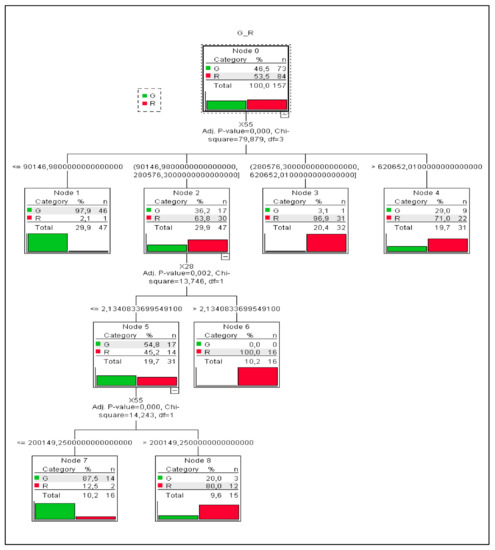
Figure 1.
Tree diagram, CHAID algorithm, 91 variables (X1–X92 without X56), and n = 157.
It can be concluded that the developed model is a very good model. This is evidenced by two obtained values. The first is risk assessment. The risk estimate is a measure of within-node variance and is used as a criterion of model fit. Lower values indicate a better model. In the case of the CHAID algorithm, a risk estimate value equal to 0.204 in cross-validation indicates a good enough model. The second value is the percentage of correctly classified enterprises. For the CHAID algorithm, 82.2% of “green” enterprises and 96.4% of “red” enterprises are correctly classified (Table 3).
Table 3.
Percentage of correctly classified enterprises, growing algorithm: CHAID, dependent variable: X93–R (red)/G (green), n = 157, 25-fold cross-validation.
In the CRT algorithm, the tree is two deep with five nodes and three terminal nodes. The method used 87 variables on 91 ratios that were calculated for the study. The first division was made in a manner similarly to that of the CHAID algorithm on the basis of the X55 ratio—working capital—at 30.6% with the values of this ratio less than or equal to 99,846.48 and 69.4% for the X55 values greater than 99,846.48. A further division occurred on the basis of X6, the ratio of retained earnings to total assets with 10.8% for values ≤ 0.015 and 56.6% for values greater than 0.015 (Figure 2).
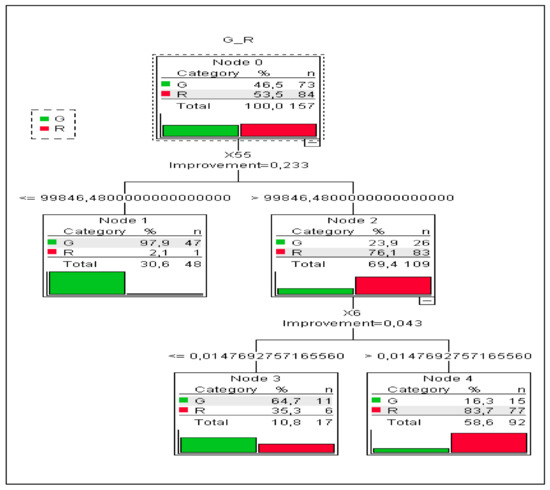
Figure 2.
Tree diagram, CRT algorithm, 91 variables (X1–X92 without X56), and n = 157.
Similar to the CHAID algorithm, this algorithm obtained very good results in both the estimation of the risk of model fit and the correct classification of enterprises. A risk value of 0.172 (Risk Estimate) when cross-validated indicates a well-fitting model. For the CRT algorithm, the percentages of the correct classification are slightly worse than the values for the CHAID algorithm, but they still show a very good result. “Green” enterprises are classified correctly in 79.5% of cases and “red” enterprises, in 91.7% (Table 4).
Table 4.
Percentage of correctly classified enterprises, growing algorithm: CRT, dependent variable: X93–R (red)/G (green), n = 157, 25-fold cross-validation.
Additionally, the classification using the k-Nearest Neighbors method was performed. An additional variable was used as the independent variable X94 (0—“green” company/1—“red” company). The aim, as in the case of the use of classification trees, was to check whether, on the basis of economic ratios specified in the database, the k-Nearest Neighbors method will correctly identify the “green” and “red” enterprises indicators. Exactly, 91 independent variables (X1–X92 without X56) and 157 records were used for the analysis. The number of k-nearest neighbors with k = 3 and the Euclidean metric as distance computation were determined. In order to validate the classification process, we divided the research sample into training and holdout partitions of 70% and 30%, respectively. Finally, the algorithm drew upon a training sample of 115 records (73.2%) and a holdout sample of 42 records (26.8%). As a result of the algorithm, for the calculation parameters defined in this way, very good results of the correct classification were obtained. In the training group, 75.9% of “green” enterprises and 91.2% of “red” enterprises were correctly classified. In the holdout sample, 86.7% “green” enterprises and 96.3% “red” enterprises were correctly classified (Table 5).
Table 5.
Percentage of correctly classified enterprises, method: k-Nearest Neighbors, dependent variable: X94: 1 (red)/0 (green), n = 157.
3.2. Altman’s Model Analysis and T-Test Sample Comparisons
In this section, Altman’s model is estimated, followed by the estimation of a modified version (re-estimation of coefficients of ratios). The T-test is then applied to ratios of “green” and “red” enterprises. The analysis uses individual years. The results for the Altman’s original model are presented in Figure 3.
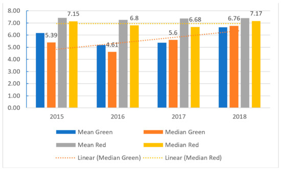
Figure 3.
The results of Altman model for emerging markets (in values).
Based on the results of the Altman model, we can determine that there are differences in the values of the model for “green” and “red” companies. These differences increase between 2015 and 2016. However, between 2017 and 2018, they decrease suggesting that the performance of green companies improves from 2016, whereas the performance of red deteriorates from 2015 onwards, with an exception for 2018. Considering bond ratings, ratings for red corporations tend to an AA rating. In contrast, green companies’ ratings tend to be a rating of BBB. This means that for investors is better to invest in “red” group of companies.
It is worth noting that this is a general model for emerging countries and based upon the results, the model did not distinguish companies from group “green” and “red” as can be seen in 2018. Therefore, we modify the original model (11) using panel data (training sample and verifying on test sample using 25-fold cross-validation). Input ratios remain the same, but estimated coefficients are different.
Z”’ = −0.81 + (8.14 × A) + (4.33 × B) − (5.56 × C) − (0.76 × D).
Model values above zero are characteristic of “red” enterprises, while values for “green” enterprises are below zero (see Figure 4). It is worth noting that, as in the original model (11), the ratio C is characterized by the highest coefficient but is negative. When analyzing the values of this ratio for “green” and “red” enterprises, it should be noted that “green” enterprises are characterized by lower values of this ratio.
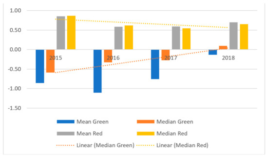
Figure 4.
The results of modified Altman model for emerging markets (in values).
The results of the re-estimation of the Altman model show that there are larger differences in values for “green” and “red” companies in comparison to the application of the original Altman, especially in 2015 but less so in 2018. There is an upward trend for “green” companies, which means that “green” companies are characterized by improving financial performance. In turn, there is a downward trend for “red” companies, with the exception for 2018, suggesting that that “red” companies are characterized by deteriorating performance. Moreover, it should be empathized that there are big differences between mean values for the “green” group and for median values. This means that some “green” enterprises are characterized by weaker financial performance relative to the rest of the firms in the green group. Given these results, we conclude that if a model with parameters for another country is used, the parameters of the model must be re-estimated for a specific country and sector.
Based upon the results of the Classification Trees and the Altman model analysis, it can be seen that the values of some of ratios discriminate against companies from the “green” and “red” groups. Therefore, we apply the Student’s t-test to 91 ratios to determine the number of ratios that can be useful (can discriminate companies between the two groups) in the analysis of these two groups of companies (see Table 6). Prior to testing, outliers are identified and removed as well as compared pairwise for missing values.
Table 6.
Summary of results of Student’s t-test, 2015–2018, and panel data.
Based on results of the Student’s t-test, it can be said that values of means for three ratios differ significantly between red and green groups over the entire sample period. The first, X29, is the logarithm of total assets, which measure the size of company. The second, X53, is the ratio of equity to fixed assets. The third ratio, X55, is net working capital. It is the excess of the company’s current assets remaining after deducting current liabilities. We analyze these ratios in more detail in the next subsection.
3.3. Analysis of Crucial Ratios
Table 7 shows the results of crucial ratios in each analysis. From analyzing the results presented in Table 7, it can be seen that only 5 ratios can be termed as crucial in each performed analysis type and only two of five are crucial in more than one type of analysis. We further discuss each separately, dividing ratios into those that featured more than once in the analysis and those that featured only once (see Figure 5, Figure 6, Figure 7, Figure 8 and Figure 9).
Table 7.
Summary of results of crucial ratios in each analysis.
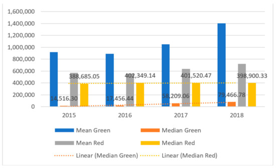
Figure 5.
The results of values of net working capital (X55) in the period of 2015–2018 and panel data (in thousands USD).
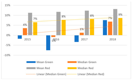
Figure 6.
The results of values of retained earnings to total assets ratio (X6) in the period of 2015–2018 and panel data (in %).
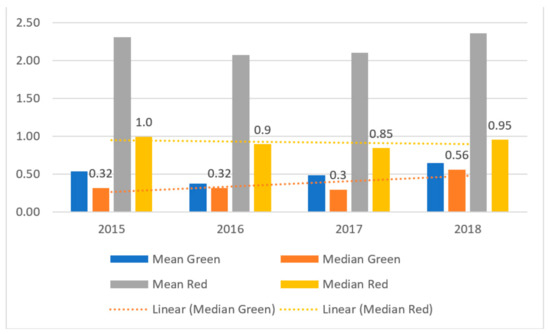
Figure 7.
The results of values of the size of net working capital (X28) in the period of 2015–2018 and panel data.
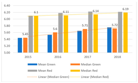
Figure 8.
The results of values of the size of company ratio (X29) in the period of 2015–2018 and panel data.
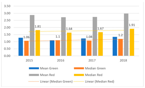
Figure 9.
The results of values for the ratio of equity to fixed assets (X53) in the period over 2015–2018 and panel data (in values).
The first ratio is net working capital (X55). This ratio belongs to liquidity ratios. The extent to which a business is secured against unforeseen expenses is dependent upon this ratio. A lack of financial liquidity signals that a business may have problems with the timely payment of current liabilities. For this reason, an appropriate level of working capital is important for a company applying for a loan or credit from the bank. This ratio can take on three values; it can be zero, greater than zero, or negative. Values above zero are considered to be favorable. The exact value of this ratio should be compared to that of the industry (see Figure 5).
A comparing of the values for X55, we note that there are notable statistically significant differences in the mean and median values for green and red companies. The median for red companies is approximately about 400,000, and for green companies, it ranges between 15,000 and 80,000. Red companies exhibit moderate downward trend, whereas green companies exhibit a notable upward trend for net working capital. Green companies exhibit values that are 5–12 times lower relative to those of red companies, although networking capital value increase over time. Moreover, a number of green companies exhibit large net working capital values. Overall, we note that there are large differences between the mean and median values within the green group of companies.
Second presented ratio is retained earnings to total assets ratio (X6). This ratio is a profitability ratio measuring retained earnings to total assets. This ratio is also indicative of a company’s leverage. Enterprises characterized by the high values finance their assets by retaining profits rather than borrowing (see Figure 6). Altman uses this ratio for the purpose of bankruptcy prediction.
We also note that there are significant differences in the mean and median values for green and red companies but not over the entire sample period. The median for red companies is approximately 8%, and for green companies, it ranges between 0% and 7%. There is a slight upward trend for “red” companies, and there is a significant upward trend for “green” companies in the period of 2016–2018. The situation is similar to that for X55; values increase substantially over the period of 2016–2018. If this upward trend continues, this ratio will be greater overall for green companies relative to that fore red companies.
The third ratio is the ratio of working capital to fixed assets, X28. High values of this ratio indicate the utilization of working capital in fixed assets and high financial liquidity (see Figure 7). Conversely, low values of the ratio may be indicative of poor performance in current activity as a consequence of the low utilization of productive capacity, excess of fixed resources, and/or overinvestment. Notably, the value of this ratio is influenced by the consumption of fixed assets.
An analysis of X28 values suggests that similar to the working capital, the “red” companies are characterized by higher values of this ratio, which means that they are described by higher liquidity. With the exception for 2018, X28 levels decline for both type of enterprises, suggesting that liquidity is decreasing.
The fourth ratio is the natural logarithm of total assets (X29)—a proxy for firm size (see Figure 8). It is assumed that the smaller a firm is, the greater the risk of bankruptcy.
Figure 8 reveals an upward trend for both groups of companies indicating an increase in the assets of the enterprises in the sector, although green companies are still smaller in terms of assets relative to red businesses.
The next ratio is the equity to fixed asset ratio (X53). This ratio verifies the fulfillment of the golden balance sheet rule, which states that fixed assets—long-term assets characterized by a low degree of liquidity—should be financed by equity, which is assumed to be a stable source of financing at the disposal of an enterprise. The fulfillment of this rule indicates a favorable financial position in terms of long-term financial stability and solvency. It also contributes to a favorable assessment of the company’s creditworthiness (see Figure 9).
For both groups, the means and medians for X53 are greater than 1. This means that the golden balance sheet rule is fulfilled. Moreover, there is an upward trend in this ratio for red companies from 2016. For green companies, no such trend is observed, only minor fluctuations in values.
4. Discussion
The findings of our study fill the gap in the discussion about the profitability of the semiconductor and related device manufacturing sector and contribute to previous research on the topic by [30]:
- extending the sample period, taking into account the period of 2015–2018, and including businesses operating in Taiwan,
- increasing the number of ratios considered to 92 and by taking not only into account ratios and variables calculated using balance sheet and profit and loss account data but also cash flow and market value data,
- using the k-Nearest Neighbors approach, Altman model, and Student’s t-test to investigate whether companies that manufacture solar modules, solar cells, solar silicon rods, solar wafers, solar power, solar photovoltaic products, and related equipment (green companies) can be differentiated from other enterprises in the sector that are not associated with renewable energy and whether these companies are in a better financial state.
Our results indicate that that green and red companies can be classified with 86%, 90%, and 93% accuracy according to the CRT, CHAID algorithms, and k-Nearest Neighbors method, respectively. These results are promising and show an improvement upon previous results where a maximum accuracy of 84% was achieved. On the basis of an assessment of the financial performance of enterprises using two variants of the Altman model, we conclude that red enterprises perform better financially relative to green enterprises. Such a finding is similar to those of [17,27,28] who suggest that going green does not pay and/or that fossil fuel companies tend to perform better financially. This finding is also in line with that of [30] who suggests that investing in green companies is not lucrative. However, green enterprises exhibit an upward trend in ratios, as indicated by an analysis of crucial ratios (see Altman model and ratios X6, X29, and X55). Such a finding offers a glimmer of hope and differs from the findings of [29] who report a fluctuating trend that is generally not strongly positive for returns on equity for RES companies. This finding implies that in the near future, financial indicators for green companies may equal or exceed those of red companies, if this upward trend continues. Furthermore, this suggests that this is a question of critical mass, which once reached will translate into outperformance for green companies over red companies. Importantly, this suggests that the profitability of green companies is increasing and thus, investing in green companies has the potential for profitability. Moreover, despite the consideration of additional ratios and variables constructed from cash flow and market data, none can be distinguished as crucial in individual analysis.
Our analysis has some limitations. First, the sample period spans the period of 2015 to 2018. However, owing to the small number of companies included in the green category, the calculated values of ratios from 2015 to 2018 are used as panel data (combined data from 2015 to 2018). This may influence results because we indicate different values of some ratios in the period. On the other hand, we obtained hopeful results. Second, the number of companies in the sample is limited. The initial database comprises 236 companies because of the limited availability of the data. Finally, we did not apply neural networks (NN) owing to the small number of companies in the sample. For this approach, we require a larger sample.
5. Conclusions
Our research sets out to determine whether investing in firms that produce components used in solar power generation is a money-making business by evaluating the semiconductor and related device manufacturing sector. We apply a unique approach for the sector taking into account 92 ratios derived from balance sheet, profit and loss account, cash flow, and market value data. The companies within this sector are classified into two groups, i.e., “green” companies are those for which production is related to renewable energy and “red” companies are those for which production is not related to renewable energy. We used Classification Trees, k-Nearest Neighbors, the Altman model, and T-tests to confirm the results of 25-fold cross-validation, significantly improving upon previous results (from 84% to 93%).
We also conclude that “green” companies can be distinguished from “red” companies on the basis of five ratios. These ratios suggest that for investors, it makes sense to invest in green companies, if this upward trend goes on. Therefore, in the near future, the performance of “green” companies may exceed the performance of “red” companies.
Author Contributions
Conceptualization, S.K.T. and A.S.-S.; methodology, S.K.T. and A.S.-S.; software, S.K.T. and A.S.-S.; validation, S.K.T. and A.S.-S.; formal analysis, S.K.T. and A.S.-S.; investigation, S.K.T. and A.S.-S.; resources, S.K.T. and A.S.-S.; data curation, S.K.T.; writing—original draft preparation, S.K.T., A.S.-S., and J.J.S.; writing—review and editing, S.K.T., A.S.-S., and J.J.S.; visualization, S.K.T.; supervision, S.K.T.; project administration, S.K.T.; funding acquisition, S.K.T. All authors have read and agreed to the published version of the manuscript.
Funding
This research was funded by Wrocław University of Science and Technology, financed from statutory funds.
Conflicts of Interest
The authors declare no conflict of interest.
References
- Hazboun, S.O.; Howe, P.D.; Coppock, D.L.; Givens, J.E. The politics of decarbonization: Examining conservative partisanship and differential support for climate change science and renewable energy in Utah. Energy Res. Soc. Sci. 2020, 70, 101769. [Google Scholar] [CrossRef]
- The International Energy Agency. Available online: https://www.iea.org/statistics (accessed on 30 October 2019).
- Independent Evaluation Group. CHINA Renewable Energy Scale-Up Program: Phase One, Report No. 117156. 2017. Available online: https://ieg.worldbankgroup.org/sites/default/files/Data/pparchinarenewableenergy-10302017.pdf (accessed on 22 December 2019).
- National Institute of Transforming India. Report of Expert Group on 175 GW RE by 2022. 2015. Available online: https://niti.gov.in/writereaddata/files/175-GW-Renewable-Energy.pdf (accessed on 22 December 2019).
- Hongzhan, S.; Qiang, Z.; Yibo, W.; Qiang, Y.; Jun, S. China’s solar photovoltaic industry development: The status quo, problems and approaches. Appl. Energy 2014, 118, 221–230. [Google Scholar]
- Pablo-Romero, M.P. Solar Energy: Incentives to Promote PV in EU27. AIMS Energy 2013, 1, 28–47. [Google Scholar] [CrossRef]
- Solangi, K.H.; Islam, M.R.; Saidur, R.; Fayaz, H.R. A review on global energy policy. Renew. Sustain. Energy Rev. 2011, 15, 2149–2163. [Google Scholar] [CrossRef]
- Sachu, B.K. A study on global solar PV energy developments and policies with a special focus on the top ten solar PV power producing countries. Renew. Sustain. Energy Rev. 2015, 43, 621–634. [Google Scholar]
- Trück, S.; Weron, R. Convenience yields and risk premiums in the EU-ETS—Evidence from the Kyoto commitment period. J. Futures Mark. 2016, 36, 587–611. [Google Scholar] [CrossRef]
- Bohl, M.T.; Kaufmann, P.; Stephan, P.M. From hero to zero: Evidence of performance reversal and speculative bubbles in German renewable energy stocks. Energy Econ. 2013, 37, 40–51. [Google Scholar] [CrossRef]
- Henriques, I.; Sadorsky, P. Oil prices and the stock prices of alternative energy companies. Energy Econ. 2008, 30, 998–1010. [Google Scholar] [CrossRef]
- Inchauspe, J.; Ripple, R.D.; Truck, S. The dynamics of returns on renewable energy companies: A state-space approach. Energy Econ. 2015, 48, 325–335. [Google Scholar] [CrossRef]
- Kumar, S.; Managi, S.; Matsuda, A. Stock prices of clean energy firms, oil and carbon markets: A vector autoregressive analysis. Energy Econ. 2012, 34, 215–226. [Google Scholar] [CrossRef]
- Managi, S.; Okimoto, T. Does the price of oil interact with clean energy prices in the stock market? Jpn. World Econ. 2013, 27, 1–9. [Google Scholar] [CrossRef]
- Maryniak, P.; Trück, S.; Weron, R. Carbon pricing and electricity markets—The case of the Australian Clean Energy Bill. Energy Econ. 2019, 79, 45–58. [Google Scholar] [CrossRef]
- Clarkson, P.M.; Li, Y.; Richardson, G.D.; Vasvari, F.P. Does it really pay to be green? Determinants and consequences of proactive environmental strategies. J. Account. Public Policy 2011, 30, 122–144. [Google Scholar] [CrossRef]
- Ruggiero, S.; Lehkonen, H. Renewable energy growth and the financial performance of electric utilities: A panel data study. J. Clean. Prod. 2017, 142, 3676–3688. [Google Scholar] [CrossRef]
- Sueyoshi, T.; Goto, M. Can environmental investment and expenditure enhance financial performance of US electric utility firms under the Clean Air Act amendment of 1990? Energy Policy 2009, 37, 4819–4826. [Google Scholar] [CrossRef]
- Telle, K. “It pays to be green”—A premature conclusion? Environ. Resour. Econ. 2006, 35, 195–220. [Google Scholar] [CrossRef]
- Pätäri, S.; Arminen, H.; Tuppura, A.; Jantunen, A. Competitive and responsible? The relationship between corporate social and financial performance in the energy sector. Renew. Sustain. Energy Rev. 2014, 37, 142–154. [Google Scholar] [CrossRef]
- Arslan-Ayaydin, Ö.; Thewissen, J. The financial reward for environmental performance in the energy sector. Energy Environ. 2016, 27, 389–413. [Google Scholar] [CrossRef]
- Sueyoshi, T.; Goto, M. Data envelopment analysis for environmental assessment: Comparison between public and private ownership in petroleum industry. Eur. J. Oper. Res. 2012, 216, 668–678. [Google Scholar] [CrossRef]
- Jamasb, T.; Pollitt, M.; Triebs, T. Productivity and eciency of US gas transmission companies: A European regulatory perspective. Energy Policy 2008, 36, 3398–3412. [Google Scholar] [CrossRef]
- Doumpos, M.; Andriosopoulos, K.; Galariotis, E.; Makridou, G.; Zopounidis, C. Corporate failure prediction in the European energy sector: A multicriteria approach and the e_ect of country characteristics. Eur. J. Oper. Res. 2017, 262, 347–360. [Google Scholar] [CrossRef]
- Bobinaite, V. Financial sustainability of wind electricity sectors in the Baltic States. Renew. Sustain. Energy Rev. 2015, 47, 794–815. [Google Scholar] [CrossRef]
- Halkos, G.E.; Tzeremes, N.G. Analyzing the Greek renewable energy sector: A Data Envelopment Analysis approach. Renew. Sustain. Energy Rev. 2012, 16, 2884–2893. [Google Scholar] [CrossRef]
- Paun, D. Sustainability and financial performance of companies in the energy sector in Romania. Sustainability 2017, 9, 1722. [Google Scholar] [CrossRef]
- Tomczak, S.K. Comparison of the Financial Standing of Companies Generating Electricity from Renewable Sources and Fossil Fuels: A New Hybrid Approach. Energies 2019, 12, 3856. [Google Scholar] [CrossRef]
- Rastogi, R.; Jaiswal, R.; Jaiswal, R.K. Renewable Energy Firm’s Performance Analysis Using Machine Learning Approach. Procedia Comput. Sci. 2020, 175, 500–507. [Google Scholar] [CrossRef]
- Tomczak, S.K.; Skowrońska-Szmer, A.; Szczygielski, J.J. Is Investing in Companies Manufacturing Solar Components a Lucrative Business? A Decision Tree Based Analysis. Energies 2020, 13, 499. [Google Scholar] [CrossRef]
- Ciarreta, A.; Espinosa, M.P.; Zarraga, A. Panel Data Analysis, Encyclopedia of Law and Economics; Springer: New York, NY, USA, 2019. [Google Scholar] [CrossRef]
- Ajmani, V.B. Panel Data Analysis; John Wiley & Sons, Inc.: Hoboken, NJ, USA, 2008. [Google Scholar] [CrossRef]
- Horbach, J. Determinants of environmental innovation—New evidence from German panel data sources. Res. Policy 2008, 37, 163–173. [Google Scholar] [CrossRef]
- Polzin, F.; Migendt, M.; Täube, F.A.; Flotow, P. Public policy influence on renewable energy investments—A panel data study across OECD countries. Energy Policy 2015, 80, 98–111. [Google Scholar] [CrossRef]
- Aparicio, S.; Urbano, D.; Audretsch, D. Institutional factors, opportunity entrepreneurship and economic growth: Panel data evidence. Technol. Forecast. Soc. Chang. 2016, 102, 45–61. [Google Scholar] [CrossRef]
- Zięba, M.; Tomczak, S.K.; Tomczak, J.M. Ensemble boosted trees with synthetic features generation in application to bankruptcy prediction. Expert Syst. Appl. 2016, 58, 93–101. [Google Scholar] [CrossRef]
- Larose, D.T. Discovering Knowledge in Data. An Introduction to Data Mining, Wiley-Interscience; John Wiley & Sons, Inc.: Hoboken, NJ, USA, 2005. [Google Scholar]
- Kass, G.V. An exploratory technique for investigating large quantities of categorical data. J. R. Stat. Soc. Ser. C 1980, 29, 119–127. [Google Scholar] [CrossRef]
- Breiman, L.; Friedman, J.; Olshen, R.; Stone, C. Classification and regression trees. Classif. Regres. Trees 2017, 37, 237–251. [Google Scholar]
- Altman, E.I.; Iwanicz-Drozdowska, M.; Laitinen, E.K.; Suvas, A. Financial distress prediction in an international context: A review and empirical analysis of Altman’s Z-score model. J. Int. Financ. Manag. Account. 2017, 28, 131–171. [Google Scholar] [CrossRef]
- Altman, E.I.; Hotchkiss, E. Corporate Financial Distress and Bankruptcy, 3rd ed.; John Wiley & Sons: Hoboken, NJ, USA, 2006. [Google Scholar]
Publisher’s Note: MDPI stays neutral with regard to jurisdictional claims in published maps and institutional affiliations. |
© 2021 by the authors. Licensee MDPI, Basel, Switzerland. This article is an open access article distributed under the terms and conditions of the Creative Commons Attribution (CC BY) license (https://creativecommons.org/licenses/by/4.0/).