Non-Equilibrium Thermodynamics-Based Convective Drying Model Applied to Oblate Spheroidal Porous Bodies: A Finite-Volume Analysis

Abstract

Commonly based on the liquid diffusion theory, drying theoretical studies in porous materials has been directed to plate, cylinder, and sphere, and few works are applied to non-conventional geometries. In this sense, this work aims to study, theoretically, the drying of solids with oblate spheroidal geometry based on the thermodynamics of irreversible processes. Mathematical modeling is proposed to describe, simultaneously, the heat and mass transfer (liquid and vapor) during the drying process, considering the variability of the transport coefficients and the convective boundary conditions on the solid surface, with particular reference to convective drying of lentil grains at low temperature and moderate air relative humidity. All the governing equations were written in the oblate spheroidal coordinates system and solved numerically using the finite-volume technique and the iterative Gauss–Seidel method. Numerical results of moisture content, temperature, liquid, vapor, and heat fluxes during the drying process were obtained, analyzed, and compared with experimental data, with a suitable agreement. It was observed that the areas near the focal point of the lentil grain dry and heat up faster; consequently, these areas are more susceptible to the appearance of cracks that can compromise the quality of the product. In addition, it was found that the vapor flux was predominant during the drying process when compared to the liquid flux.

1. Introduction

Water is the main constituent present in high concentrations in fresh foods, which considerably influences the palatability, digestibility, and physical structure of the food. The deterioration that occurs in food is practically influenced in one way or another by the concentration and mobility of water inside it [1]. The removal of water from solid foods is used as a way to reduce water activity by inhibiting microbial growth, thus avoiding its deterioration. Water removal has become of great importance in reducing the costs of energy, transport, packaging, and storage of these foods [2].

Most of the methods of food preservation are based on the reduction in water mobility by the use of humectants materials and freezing, and also by physical removal of water through osmotic dehydration, drying, evaporation, or lyophilization [3]. The main idea is to decrease the amount of water in the product to acceptable levels and maintain the physical-chemical and sensory properties of agricultural products in order to increase the shelf life of the products.

Although several technological processes of food conservation can be applied in order to increase the shelf life of agricultural products, the drying process has several advantages, as: the facility in the preservation of the product; stability of aromatic components at room temperature for long periods of time; protection against enzymatic and oxidative degradation; reducing of the weight; energy savings because it does not require refrigeration and product availability during any time of the year [4]. In literature, it is possible to find several studies that showed the use of drying processes as a method to increase the shelf life of products such as: lentils [5,6]; grape [7]; carrots [8]; banana [9]; corn [10,11]; red chilies [12]; wheat [13]; bean [14]; strawberry [15], etc.

Drying is a unitary operation of water removal of a product by evaporation or sublimation, by applying heat under controlled conditions, which has, as its purpose, to conserve food and its nutritional and organoleptic properties by reducing the activity of water inside it [16].

During the drying process, the material undergoes variations in its chemical, physical and biological characteristics, which, depending on the intensity of the effect, may cause their loss or disable them for some applicability [7,17]. Thus, the criterion of preserving the quality of the product, which depends on the final use that will be made, is the one that regulates the type of drying and storage process [2].

From the theoretical point of view, the modeling and prediction of the drying process can be approached in two ways: based on external parameters to the solid such as relative humidity, temperature, and air velocity, correlating them with the drying rate of the solid, while the other has as characteristic, the internal conditions to the porous material and the mechanisms of moisture transport in this material [18].

The complexity of drying leads several researchers to propose various theories and models to predict the moisture transfer inside the material, such as: liquid diffusion theory, capillary theory, condensation and evaporation theory, Luikov theory, Krischer theory, Berger and Pei theory, Philip and De Vries theory, and the theory of Fortes and Okos [19].

The Luikov model [20] and Fortes and Okos [19] model are examples of models based on the thermodynamics of irreversible processes. Luikov’s theory takes into account the mechanisms of diffusion, effusion, and convection of water inside the porous medium. Therefore, the equations that define the Luikov model take into account that the molecular transport of water vapor, air, and liquid happen simultaneously [21]. On the other hand, Fortes [22] and Fortes and Okos [19,23] proposed that the driving force for isothermal transfer, both liquid and vapor, is the gradient of equilibrium moisture content, due to the local equilibrium hypothesis, which, in turn, is a function of temperature, relative humidity, and equilibrium moisture content. Detail about the non-equilibrium thermodynamic can be found in the references cited in the text.

Oliveira and Lima [24] used the model proposed by Fortes and Okos [19] to study the heat and mass transfer in the simulation of wheat drying and concluded that the numerical results of the average moisture content showed a suitable agreement with the experimental values. Oliveira et al. [25] and Oliveira et al. [26] observed, applying the model developed by Fortes and Okos [19] to study the phenomenon of shrinkage during a drying process of wheat grain, that the model used was accurate and effective and could be used to simulate many practical diffusion problems, such as heating, cooling, wetting and drying in prolate spheroidal solids, including spherical solids.

In previous studies, Carmo and Lima [27] reported studies of drying of oblate spheroidal porous solids using the liquid diffusion theory, with particular reference to lentil grains, considering constant thermophysical properties and equilibrium, and convective boundary conditions on the solid surface. Melo et al. [28] and Melo et al. [29] reported the transient behavior of heat and mass transfer, also in oblate spheroidal solids (lentil grains) using a mathematical model based on the thermodynamics of irreversible processes and considering equilibrium boundary condition on the surface of the solid. In this study, the authors reported vapor flux as the dominant mechanism for mass transfer during the drying process.

In this sense, due to the fact that few works studied coupled heat and mass transfer in solids with complex shape [18,24,25,26,27]; that during the drying process of agricultural products with low moisture content, the predominant mass flux is the vapor flux (not predicted by the liquid diffusion theory l), and the equilibrium boundary condition (hygroscopic and thermal balances) does not accurately reflect the physical phenomenon of heat and mass transport on the surface of the grain; this work aims to study the transfer of heat and mass in oblate spheroidal porous materials using mathematical modeling based on the non-equilibrium thermodynamics. This model considers variable thermophysical properties and convective boundary conditions on the surface of the porous solid. The application has been given for lentil grains drying. The idea is to provide subsidies for a better understanding of the drying process in solids with complex shapes in order to allow its optimization in terms of energy consumption (prediction of drying time) and product quality (evaluated by the moisture and heat transfer inside the hygroscopic porous solid).

2. Methodology

2.1. Mathematical Modeling

The model under study involves the determination of heat and mass transfer in a two-dimensional case for solids with ellipsoidal geometry. In the mathematical formulation, the following assumptions were adopted:

(a)

The solid is homogeneous and isotropic;

(b)

Mass transfer in the single particle occurs by diffusion of liquid and vapor, under decreasing drying rate;

(c)

At the beginning of the drying process, the distributions of the moisture and temperature content are considered uniform and symmetrical around the z-axis;

(d)

The thermophysical properties are variable during the drying process and dependent on the position and moisture content inside the material;

(e)

Volume shrinkage negligible;

(f)

No capillarity effect;

(g)

Moisture transfer inside the solid by liquid and vapor diffusion, and evaporation and convection on a solid surface;

(h)

Heat transfer inside the solid by conduction, evaporation, and convection on a solid surface.

Based on a mechanistic approach and considering equality between the chemical potential and the potential of water (suction), Fortes [22], Fortes and Okos [23], and Fortes and Okos [19] reported a set of partial differential equations to describe the drying process of porous hygroscopic solids. According to these authors, the expression that describes the liquid flux is given by:

$${\overrightarrow{\mathrm{J}}}_{\ell }=-{\mathsf{\rho }}_{\ell }{\mathrm{k}}_{\ell }{\mathrm{R}}_{\mathrm{v}}\ell \mathrm{nH}\nabla \mathrm{T}-{\mathsf{\rho }}_{\ell }{\mathrm{k}}_{\ell }\left(\frac{{\mathrm{R}}_{\mathrm{v}}\mathrm{T}}{\mathrm{H}}\right)\frac{\partial \mathrm{H}}{\partial \mathrm{M}}\nabla \mathrm{M}+{\mathsf{\rho }}_{\ell }{\mathrm{k}}_{\ell }\overrightarrow{\mathrm{g}}$$

(1)

where ρ_l is the liquid density, k_l is the liquid conductivity, H is the relative humidity, T is the temperature, M is the moisture content, R_v is the universal gas constant, and g is the acceleration of gravity.

The expression that describes the vapor flux is given by:

$${\overrightarrow{\mathrm{J}}}_{\mathrm{v}}=-{\mathrm{k}}_{\mathrm{v}}\left({\mathsf{\rho }}_{\mathrm{v}0}\frac{\partial \mathrm{H}}{\partial \mathrm{T}}+\mathrm{H}\frac{\mathrm{d}{\mathsf{\rho }}_{\mathrm{v}0}}{\mathrm{d}\mathrm{T}}\right)\nabla \mathrm{T}-{\mathrm{k}}_{\mathrm{v}}{\mathsf{\rho }}_{\mathrm{v}0}\frac{\partial \mathrm{H}}{\partial \mathrm{M}}\nabla \mathrm{M}+{\mathsf{\rho }}_{\mathrm{l}}{\mathrm{k}}_{\mathrm{l}}\overrightarrow{\mathrm{g}}$$

(2)

where k_v is the vapor conductivity and ρ_v0 is the saturation density. The heat flux is given by the following equation:

$$\begin{array}{ll}{\overrightarrow{\mathrm{J}}}_{\mathrm{q}}=& -{\mathrm{k}}_{\mathrm{T}}\nabla \mathrm{T}-\left[{\mathsf{\rho }}_{\ell }{\mathrm{k}}_{\ell }{\mathrm{R}}_{\mathrm{v}}\ell \mathrm{nH}+{\mathrm{k}}_{\mathrm{v}}\left({\mathsf{\rho }}_{\mathrm{v}0}\frac{\partial \mathrm{H}}{\partial \mathrm{T}}+\mathrm{H}\frac{\mathrm{d}{\mathsf{\rho }}_{\mathrm{v}0}}{\mathrm{dT}}\right)\right]\frac{{\mathrm{R}}_{\mathrm{v}}{\mathrm{T}}^2}{\mathrm{H}}\frac{\partial \mathrm{H}}{\partial \mathrm{M}}\nabla \mathrm{M}+\\ & +\mathrm{T}\left[{\rho }_{\ell }{\mathrm{k}}_{\ell }{\mathrm{R}}_{\mathrm{v}}\ell \mathrm{nH}+{\mathrm{k}}_{\mathrm{v}}\left({\mathsf{\rho }}_{\mathrm{v}0}\frac{\partial \mathrm{H}}{\partial \mathrm{T}}+\mathrm{H}\frac{\mathrm{d}{\mathsf{\rho }}_{\mathrm{v}0}}{\mathrm{dT}}\right)\right]\overrightarrow{\mathrm{g}}\end{array}$$

(3)

where k_T is the effective apparent thermal conductivity of the porous medium, valid for conditions that do not involve mass transport.

Considering the absence of ice and that several factors are negligible, as the air mass, the vapor mass (but not its flux) in relation to the liquid mass and shrinkage of the medium, the differential equation for the mass transfer in the vapor and liquid phases inside the material, and applied to an elementary control volume, is given as follows:

$${\mathsf{\rho }}_{\mathrm{s}}\frac{\partial \mathrm{M}}{\partial \mathrm{t}}=-\nabla \cdot \left({\overrightarrow{\mathrm{J}}}_{\ell }+{\overrightarrow{\mathrm{J}}}_{\mathrm{v}}\right),$$

(4)

where t is the time and M = M_ℓ + M_v ≅ M_ℓ.

The energy balance equation could be obtained by the relation between the rate of variation of the volumetric enthalpy of the system and the adsorption heat with the divergence of the enthalpy flux (liquid and vapor phases),

$$\frac{\partial }{\partial \mathrm{t}}\left({\mathsf{\rho }}_{\mathrm{s}}{\mathrm{c}}_{\mathrm{b}}\mathrm{T}\right)-\frac{\partial }{\partial \mathrm{t}}\left({\mathsf{\rho }}_{\mathrm{s}}{\mathrm{h}}_{\mathrm{w}}\mathrm{M}\right)=-\nabla \cdot {\overrightarrow{\mathrm{J}}}_{\mathrm{q}}-\nabla \cdot \left({\mathrm{h}}_{\mathrm{fg}}{\overrightarrow{\mathrm{J}}}_{\mathrm{v}}\right)-{\overrightarrow{\mathrm{J}}}_{\ell }\cdot {\mathrm{c}}_{\ell }\nabla \mathrm{T}-{\overrightarrow{\mathrm{J}}}_{\mathrm{v}}\cdot {\mathrm{c}}_{\mathrm{v}}\nabla \mathrm{T}$$

(5)

where h_w is the differential specific heat of sorption, h_fg is the specific latent heat of water vaporization, and c_b is the specific heat of the humid medium, given by:

$${\mathrm{c}}_{\mathrm{b}}={\mathrm{c}}_{\mathrm{s}}+{\mathrm{c}}_{\ell }{\mathrm{M}}_{\ell }+{\mathrm{c}}_{\mathrm{v}}{\mathrm{M}}_{\mathrm{v}}$$

(6)

where c_s is the specific heat of the dry product, c_l is the specific heat of the liquid, and c_v is the vapor specific heat.

Furthermore, considering the gravitational effects, Equations (4) and (5) could be written in a more compact form as,

$$\frac{\partial }{\partial \mathrm{t}}\left({\mathsf{\rho }}_{\mathrm{s}}\mathrm{M}\right)=\nabla \cdot \left({\Gamma }_1^{\Phi }\nabla \mathrm{M}\right)+\nabla \cdot \left({\Gamma }_2^{\Phi }\nabla \mathrm{T}\right),$$

(7)

and

$$\begin{gathered} \frac{\partial }{\partial \mathrm{t}}\left({\mathsf{\rho }}_{\mathrm{s}}{\mathrm{c}}_{\mathrm{b}}\mathrm{T}\right)-\frac{\partial }{\partial \mathrm{t}}\left({\mathsf{\rho }}_{\mathrm{s}}{\mathrm{h}}_{\mathrm{w}}\mathrm{M}\right)=\nabla \cdot \left({\mathsf{\Gamma }}_3^{\mathsf{\Phi }}\nabla \mathrm{T}\right)+\nabla \cdot \left({\mathsf{\Gamma }}_4^{\mathsf{\Phi }}\nabla \mathrm{M}\right)+\nabla \cdot \left({\mathsf{\Gamma }}_5^{\mathsf{\Phi }}\nabla \mathrm{T}\right) \\ +\nabla \cdot \left({\mathsf{\Gamma }}_6^{\mathsf{\Phi }}\nabla \mathrm{M}\right)+{\mathsf{\Gamma }}_7^{\mathsf{\Phi }}\nabla \mathrm{T}\cdot \nabla \mathrm{T}+{\mathsf{\Gamma }}_8^{\mathsf{\Phi }}\nabla \mathrm{M}\cdot \nabla \mathrm{T}, \end{gathered}$$

(8)

where the parameter ${\mathsf{\Gamma }}_{\mathrm{i}}^{\mathsf{\Phi }}$ is given in Appendix A.

In this work, a porous solid with oblate spheroidal geometry was considered. Figure 1 shows half of the solid and some geometric parameters of this body. In this figure, μ, φ and ω represent the elliptical coordinates, and L₁ and L₂ are the minor and major axis of the ellipse.

In order to present the diffusion equation in an oblate spheroidal coordinates system, the following relationships are used [30]:

$$\mathrm{x}=\mathrm{L}\sqrt{\left(1+{\mathsf{\xi }}^2\right)\left(1-{\mathsf{\eta }}^2\right)} \mathsf{\zeta },$$

(9)

$$\mathrm{y}=\mathrm{L}\sqrt{\left(1+{\mathsf{\xi }}^2\right)\left(1-{\mathsf{\eta }}^2\right)}\sqrt{1-{\mathsf{\zeta }}^2},$$

(10)

$$\mathrm{z}=\mathrm{L}\mathsf{\xi } \mathsf{\eta },$$

(11)

where ξ = sinh µ, η = cos φ and ζ = cos ϖ. Finally, L is the focal length given by:

$$\mathrm{L}\hspace{0.17em}=\hspace{0.17em}\sqrt{{\mathrm{L}}_2^2\hspace{0.17em}-\hspace{0.17em}{\mathrm{L}}_1^2}.$$

(12)

The domain of the new spheroidal variables ξ, η and ζ (in terms of ω), related with Figure 1 is given by: 0 ≤ ξ ≤ L₁/L, 0 ≤ η ≤ 1 and 0 ≤ ω ≤ 2π.

Using the methodology described by Maliska [31] in order to obtain the diffusion equation in the oblate spheroidal coordinates system and, considering the symmetry of the solid, the following diffusion equations for the two-dimensional case are obtained:

$$\begin{gathered} \frac{\partial \hspace{0.17em}\left({\mathsf{\rho }}_{\mathrm{s}}\mathrm{M}\right)}{\partial \hspace{0.17em}\mathrm{t}}=\left[\frac{1}{{\mathrm{L}}^2\left({\mathsf{\xi }}^2+{\mathsf{\eta }}^2\right)}\frac{\partial }{\partial \mathsf{\xi }}\left(\left({\mathsf{\xi }}^2+1\right){\Gamma }_1{}^{\Phi }\frac{\partial \mathrm{M}}{\partial \mathsf{\xi }}\right)\right]+\left[\frac{1}{{\mathrm{L}}^2\left({\mathsf{\xi }}^2+{\mathsf{\eta }}^2\right)}\frac{\partial }{\partial \mathsf{\eta }}\left(\left(1-{\mathsf{\eta }}^2\right){\Gamma }_1{}^{\Phi }\frac{\partial \mathrm{M}}{\partial \mathsf{\eta }}\right)\right] \\ +\left[\frac{1}{{\mathrm{L}}^2\left({\mathsf{\xi }}^2+{\mathsf{\eta }}^2\right)}\frac{\partial }{\partial \mathsf{\xi }}\left(\left({\mathsf{\xi }}^2+1\right){\Gamma }_2{}^{\Phi }\frac{\partial \mathrm{T}}{\partial \mathsf{\xi }}\right)\right]+\left[\frac{1}{{\mathrm{L}}^2\left({\mathsf{\xi }}^2+{\mathsf{\eta }}^2\right)}\frac{\partial }{\partial \mathsf{\eta }}\left(\left(1-{\mathsf{\eta }}^2\right){\Gamma }_2{}^{\Phi }\frac{\partial \mathrm{T}}{\partial \mathsf{\eta }}\right)\right], \end{gathered}$$

(13)

and

$$\begin{gathered} \frac{\partial }{\partial \mathrm{t}}\left({\mathsf{\rho }}_{\mathrm{s}}{\mathrm{c}}_{\mathrm{b}}\mathrm{T}\right)-\frac{\partial }{\partial \mathrm{t}}\left({\mathsf{\rho }}_{\mathrm{s}}{\mathrm{h}}_{\mathrm{w}}\mathrm{M}\right)=\frac{1}{{\mathrm{L}}^2\left({\mathsf{\xi }}^2+{\mathsf{\eta }}^2\right)}\left\{\frac{\partial }{\partial \mathsf{\xi }}\left[\left({\mathsf{\xi }}^2+1\right){\Gamma }_3^{\Phi }\frac{\partial \mathrm{T}}{\partial \mathsf{\xi }}\right]+\frac{\partial }{\partial \mathsf{\eta }}\left[\left(1-{\mathsf{\eta }}^2\right){\Gamma }_3^{\Phi }\frac{\partial \mathrm{T}}{\partial \mathsf{\eta }}\right]\right\}+ \\ \begin{array}{l}+\frac{1}{{\mathrm{L}}^2\left({\mathsf{\xi }}^2+{\mathsf{\eta }}^2\right)}\left\{\frac{\partial }{\partial \mathsf{\xi }}\left[\left({\mathsf{\xi }}^2+1\right){\Gamma }_5^{\Phi }\frac{\partial \mathrm{T}}{\partial \mathsf{\xi }}\right]+\frac{\partial }{\partial \mathsf{\eta }}\left[\left(1-{\mathsf{\eta }}^2\right){\Gamma }_5^{\Phi }\frac{\partial \mathrm{T}}{\partial \mathsf{\eta }}\right]\right\}+\frac{{\Gamma }_7^{\Phi }}{{\mathrm{L}}^2\left({\mathsf{\xi }}^2+{\mathsf{\eta }}^2\right)}\\ \left[\left({\mathsf{\xi }}^2+1\right){\left(\frac{\partial \mathrm{T}}{\partial \mathsf{\xi }}\right)}^2+\left(1-{\mathsf{\eta }}^2\right){\left(\frac{\partial \mathrm{T}}{\partial \mathsf{\eta }}\right)}^2\right]+\frac{{\Gamma }_8^{\Phi }}{{\mathrm{L}}^2\left({\mathsf{\xi }}^2+{\mathsf{\eta }}^2\right)}\left[\left({\mathsf{\xi }}^2+1\right)\frac{\partial \mathrm{M}}{\partial \mathsf{\xi }}\frac{\partial \mathrm{T}}{\partial \mathsf{\xi }}+\left(1-{\mathsf{\eta }}^2\right)\frac{\partial \mathrm{M}}{\partial \mathsf{\eta }}\frac{\partial \mathrm{T}}{\partial \mathsf{\eta }}\right]+\end{array} \\ \begin{array}{l}+\frac{1}{{\mathrm{L}}^2\left({\mathsf{\xi }}^2+{\mathsf{\eta }}^2\right)}\left\{\frac{\partial }{\partial \mathsf{\xi }}\left[\left({\mathsf{\xi }}^2+1\right){\Gamma }_4^{\Phi }\frac{\partial \mathrm{M}}{\partial \mathsf{\xi }}\right]+\frac{\partial }{\partial \mathsf{\eta }}\left[\left(1-{\mathsf{\eta }}^2\right){\Gamma }_4^{\Phi }\frac{\partial \mathrm{M}}{\partial \mathsf{\eta }}\right]\right\}+\\ +\frac{1}{{\mathrm{L}}^2\left({\mathsf{\xi }}^2+{\mathsf{\eta }}^2\right)}\left\{\frac{\partial }{\partial \mathsf{\xi }}\left[\left({\mathsf{\xi }}^2+1\right){\Gamma }_6^{\Phi }\frac{\partial \mathrm{M}}{\partial \mathsf{\xi }}\right]+\frac{\partial }{\partial \mathsf{\eta }}\left[\left(1-{\mathsf{\eta }}^2\right){\Gamma }_6^{\Phi }\frac{\partial \mathrm{M}}{\partial \mathsf{\eta }}\right]\right\}\end{array} \end{gathered}$$

(14)

Equations (13) and (14) can be rewritten as:

$$\frac{\partial }{\partial \mathrm{t}}\left(\frac{{\mathsf{\lambda }}_1{\mathsf{\Phi }}_1}{\mathrm{J}}\right)=\frac{\partial }{\partial \mathsf{\xi }}\left({\mathsf{\alpha }}_{11}\mathrm{J}\hspace{0.17em}{\mathsf{\Gamma }}_1^{\mathsf{\Phi }}\frac{\partial {\mathsf{\Phi }}_1}{\partial \mathsf{\xi }}\right)+\frac{\partial }{\partial \mathsf{\eta }}\left({\mathsf{\alpha }}_{22}\mathrm{J}\hspace{0.17em}{\mathsf{\Gamma }}_1^{\mathsf{\Phi }}\frac{\partial {\mathsf{\Phi }}_1}{\partial \mathsf{\eta }}\right)+{\mathrm{S}}_1^{\mathsf{\Phi }}$$

(15)

and

$$\begin{array}{l}\frac{\partial }{\partial \mathrm{t}}\left(\frac{{\lambda }_2{\mathsf{\Phi }}_2}{\mathrm{J}}\right)=\frac{\partial }{\partial \mathsf{\xi }}\left({\mathsf{\alpha }}_{11}\mathrm{J}{\Gamma }_3^{\mathsf{\Phi }}\frac{\partial {\mathsf{\Phi }}_2}{\partial \mathsf{\xi }}\right)+\frac{\partial }{\partial \mathsf{\eta }}\left({\mathsf{\alpha }}_{22}\mathrm{J}{\Gamma }_3^{\mathsf{\Phi }}\frac{\partial {\mathsf{\Phi }}_2}{\partial \mathsf{\eta }}\right)+\frac{\partial }{\partial \mathsf{\xi }}\left({\mathsf{\alpha }}_{11}\mathrm{J}{\Gamma }_5^{\mathsf{\Phi }}\frac{\partial {\mathsf{\Phi }}_2}{\partial \mathsf{\xi }}\right)+\\ +\frac{\partial }{\partial \mathsf{\eta }}\left({\mathsf{\alpha }}_{22}\mathrm{J}{\Gamma }_5^{\mathsf{\Phi }}\frac{\partial {\mathsf{\Phi }}_2}{\partial \mathsf{\eta }}\right)+{\mathrm{S}}_2^{\mathsf{\Phi }}\end{array}$$

(16)

where the source terms ${\mathrm{S}}_1^{\mathsf{\Phi }}$ and ${\mathrm{S}}_2^{\mathsf{\Phi }}$ are given in Appendix A.

For a well-posed formulation, the initial boundary and symmetry conditions for the proposed model are the following:

(a)

Mass

• Initial:

  M(ξ, η, t = 0) = M_o.

  (17)
• Symmetry planes: In mass transfer the angular and radial gradients of the moisture content are equal to zero in the symmetry planes.

  $$\frac{\partial \mathrm{M} \left(\mathsf{\xi },1,\mathrm{t}\right)}{\partial \mathsf{\eta }}=0$$

  (18)

  $$\frac{\partial \mathrm{M} \left(\mathsf{\xi },0,\mathrm{t}\right)}{\partial \mathsf{\eta }}=0$$

  (19)

  $$\frac{\partial \mathrm{M} \left(0,\mathsf{\eta },\mathrm{t}\right)}{\partial \mathsf{\xi }}=0$$

  (20)
• Free surface: The diffusive flux is equal to the convective flux of the moisture content on the surface of the oblate spheroid.

  $$\left({\overrightarrow{\mathrm{J}}}_{\ell }+{\overrightarrow{\mathrm{J}}}_{\mathrm{v}}\right) |{}_{\mathsf{\xi }=\frac{\mathrm{L}1}{\mathrm{L}}}={\mathrm{h}}_{\mathrm{m}}\left(\mathrm{M}-{\mathrm{M}}_{\mathrm{e}}\right) \mathrm{with} \mathrm{T}={\mathrm{T}}_{\mathrm{a}} \mathrm{and} \mathrm{H}={\mathrm{H}}_{\mathrm{a}}.$$

  (21)

(b)

Heat

• Initial

  T(ξ,η, t = 0) = T_o = cte.

  (22)
• Symmetry plane: Heat angular and radial gradients are equal to zero.

  $$\frac{\partial \mathrm{T} \left(\mathsf{\xi },1,\mathrm{t}\right)}{\partial \mathsf{\eta }}=0$$

  (23)

  $$\frac{\partial \mathrm{T} \left(\mathsf{\xi },0,\mathrm{t}\right)}{\partial \mathsf{\eta }}=0$$

  (24)

  $$\frac{\partial \mathrm{T} \left(0,\mathsf{\eta },\mathrm{t}\right)}{\partial \mathsf{\xi }}=0$$

  (25)
• Free surface: The diffusive flux is equal to the heat convective flux on the surface of the solid, more the energy to evaporate the water and the energy to heat the water vapor produced in the evaporation process. Then we can write:

  $${\overrightarrow{\mathrm{J}}}_{\mathrm{q}}|{}_{\mathsf{\xi }=\frac{{\mathrm{L}}_1}{\mathrm{L}}}={\mathrm{h}}_{\mathrm{c}}{ (\mathrm{T}}_{\mathrm{s}}-{\mathrm{T}}_{\mathrm{a}})+{\mathrm{h}}_{\mathrm{fg}}{ \mathrm{J} \to }_{\ell }+\left({\overrightarrow{\mathrm{J}}}_{\ell }+{\overrightarrow{\mathrm{J}}}_{\mathrm{v}}\right){\mathrm{c}}_{\mathrm{v}}\left({\mathrm{T}}_{\mathrm{s}}-{\mathrm{T}}_{\mathrm{a}}\right).$$

  (26)

The average moisture content of the porous body during the drying process is given by [32]:

$$\overline{\mathrm{M}}=\frac{1}{\mathrm{V}}{\displaystyle \underset{\mathrm{v}}{\int }\mathrm{M} \left(\mathsf{\xi }, \mathsf{\eta }, \mathrm{t}\right) }\mathrm{dV}.$$

(27)

The average temperature of the porous body during the drying process could be obtained as follows:

$$\overline{\mathrm{T}}=\frac{1}{\mathrm{V}}{\displaystyle \underset{\mathrm{v}}{\int }\mathrm{T} \left(\mathsf{\xi }, \mathsf{\eta }, \mathrm{t}\right) \mathrm{dV}},$$

(28)

where V is the volume of the solid.

2.2. Numerical Solution of the Governing Equations

In this work, the finite-volume method was used to numerically solve the diffusion equation in oblate spheroidal coordinates. In this method, the nodal points are centered on the control volume and the mesh adopted has entire volumes throughout the domain [31,33].

The numerical formulation adopted begins with the identification of the domain of interest and, from there, its division into a finite number of subdomains. Figure 2 shows the constant lines ξ and η delimiting the control volume associated with point nodal P. Points N, S, E, and W are the nodal points neighboring P, which represent the nodal points north, south, east, and west, respectively. The distance between the nodal point P and its neighbors (δξ and δη) is also observed, as well as the control volume dimensions (Δξ and Δη).

Applying the finite-volume method to Equations (15) and (16), considering a fully implicit formulation, i.e., all diffusive terms of the equation are evaluated at the instant t + Δt, integrating on the control volume (see Figure 2), which corresponds to the internal points of the domain for a time t, and rearranging the terms of the resulting equation, the following linear equation, for mass transfer, is obtained in the following discretized form:

$${\mathrm{A}}_1{}_{\mathrm{P}}{\mathsf{\Phi }}_{1\mathrm{P}}={\mathrm{A}}_1{}_{\mathrm{N}}{\mathsf{\Phi }}_{1\mathrm{N}}+{\mathrm{A}}_1{}_{\mathrm{S}}{\mathsf{\Phi }}_{1\mathrm{S}}+{\mathrm{A}}_1{}_{\mathrm{E}}{\mathsf{\Phi }}_{1\mathrm{E}}+{\mathrm{A}}_1{}_{\mathrm{W}}{\mathsf{\Phi }}_{1\mathrm{W}}+{\mathrm{A}}_{1\mathrm{P}}^{\mathrm{o}}{\mathsf{\Phi }}_{1\mathrm{P}}^{\mathrm{o}}+{\widehat{S}}_1^{\mathsf{\Phi }},$$

(29)

where:

$${\hat{\mathrm{S}}}_1^{\mathsf{\Phi }}={\mathrm{B}}_1{}_{\mathrm{N}}{\mathsf{\Phi }}_{2\mathrm{N}}+{\mathrm{B}}_1{}_{\mathrm{S}}{\mathsf{\Phi }}_{2\mathrm{S}}+{\mathrm{B}}_1{}_{\mathrm{E}}{\mathsf{\Phi }}_{2\mathrm{E}}+{\mathrm{B}}_1{}_{\mathrm{W}}{\mathsf{\Phi }}_{2\mathrm{W}}-{\mathrm{B}}_1{}_{\mathrm{P}}{\mathsf{\Phi }}_{2\mathrm{P}},$$

(30)

where the coefficients A_i are given in Appendix A. In Equations (29) and (30) the parameters ${\mathsf{\Phi }}_1=\mathrm{M}$ and ${\mathsf{\Phi }}_2=\mathrm{T}$.

For energy balance (${\mathsf{\Phi }}_2=\mathrm{T}$), it results in:

$${\mathrm{A}}_{2\mathrm{P}}{\mathsf{\Phi }}_{2\mathrm{P}}={\mathrm{A}}_2{}_{\mathrm{N}}{\mathsf{\Phi }}_{2\mathrm{N}}+{\mathrm{A}}_2{}_{\mathrm{S}}{\mathsf{\Phi }}_{2\mathrm{S}}+{\mathrm{A}}_2{}_{\mathrm{E}}{\mathsf{\Phi }}_{2\mathrm{E}}+{\mathrm{A}}_2{}_{\mathrm{EW}}{\mathsf{\Phi }}_{2\mathrm{W}}+{\mathrm{A}}_{2\mathrm{P}}^0{\mathsf{\Phi }}_{2\mathrm{P}}^0+{\mathrm{S}}_2^{\mathsf{\Phi }},$$

(31)

with:

$${\widehat{\mathrm{S}}}_2^{\mathsf{\Phi }}={\mathrm{S}}_{\mathrm{C}2}^{\mathsf{\Phi }}+{\mathrm{S}}_{\mathrm{P}2}^{\mathsf{\Phi }},$$

(32)

and

$$\begin{array}{l}{\mathrm{S}}_{\mathrm{P}2}^{\mathsf{\Phi }}=-\left[{\mathsf{\Gamma }}_{7\mathrm{n}}^{\mathsf{\Phi }}\left({\mathsf{\xi }}^2+1\right)\mathsf{\Delta }\mathsf{\eta }\mathsf{\Delta }\mathsf{\xi }\left(\frac{{\mathsf{\Phi }}_{2\mathrm{N}}^{\ast }-{\mathsf{\Phi }}_{2\mathrm{P}}^{\ast }}{{\mathsf{\delta }\mathsf{\xi }}_{\mathrm{n}}}\right)\right]-\left[{\mathsf{\Gamma }}_{7\mathrm{n}}^{\mathsf{\Phi }}\left(1-{\mathsf{\eta }}^2\right)\mathsf{\Delta }\mathsf{\eta }\mathsf{\Delta }\mathsf{\xi }\left(\frac{{\mathsf{\Phi }}_{2\mathrm{E}}^{\ast }-{\mathsf{\Phi }}_{2\mathrm{P}}^{\ast }}{{\mathsf{\delta }\mathsf{\eta }}_{\mathrm{e}}}\right)\right]+\\ \left[{\mathsf{\Gamma }}_{8\mathrm{n}}^{\mathsf{\Phi }}\left({\mathsf{\xi }}^2+1\right)\mathsf{\Delta }\mathsf{\eta }\mathsf{\Delta }\mathsf{\xi }\left(\frac{{\mathsf{\Phi }}_{1\mathrm{N}}-{\mathsf{\Phi }}_{1\mathrm{P}}}{{\mathsf{\delta }\mathsf{\xi }}_{\mathrm{n}}}\right)\right]+{\mathsf{\Gamma }}_{8\mathrm{e}}^{\mathsf{\Phi }}\left(1-{\mathsf{\eta }}^2\right)\mathsf{\Delta }\mathsf{\eta }\mathsf{\Delta }\mathsf{\xi }\left(\frac{{\mathsf{\Phi }}_{1\mathrm{E}}-{\mathsf{\Phi }}_{1\mathrm{P}}}{{\mathsf{\delta }\mathsf{\eta }}_{\mathrm{e}}}\right)\end{array}$$

(33)

$${\mathrm{S}}_{\mathrm{C}2}^{\mathsf{\Phi }}={\mathrm{B}}_{\mathrm{star}}+{\mathrm{B}}_{2\mathrm{N}}{\mathsf{\Phi }}_{1\mathrm{N}}+{\mathrm{B}}_{2\mathrm{S}}{\mathsf{\Phi }}_{1\mathrm{S}}+{\mathrm{B}}_{2\mathrm{E}}{\mathsf{\Phi }}_{1\mathrm{E}}+{\mathrm{B}}_{2\mathrm{W}}{\mathsf{\Phi }}_{1\mathrm{W}}-{\mathrm{B}}_{2\mathrm{P}}{\mathsf{\Phi }}_{1\mathrm{P}}-{\mathrm{B}}_{\mathrm{P}2}^{\mathrm{o}}{\mathsf{\Phi }}_{\mathrm{P}2}^{\mathrm{o}}.$$

(34)

The coefficients A_K and A⁰_P, with K ≠ P, describe the contribution of the different nodes due to the diffuse transport of (from the neighboring points in the direction of the node P) and the influence of the variable Φ in the previous time on its value at the present time, respectively.

The main advantage of the use of the implicit procedure is that it is unconditionally stable [33]; however, the use of this formulation does not mean working with any time interval because the coupling problem can limit with great intensity the value of Δt.

Equations (29) and (31) are applied to all internal points in the discrete domain, except at the border points (see Figure 3), which are the control volumes adjacent to the body surface (boundary volumes). For these volumes, the procedure adopted is the integration of conservation equations, considering the boundary conditions existing on the surface of the porous solid.

In this case, the following discretized equations are valid:

• Mass:

  $$\frac{\Delta \mathrm{V}}{{\mathrm{J}}_{\mathrm{p}}}\left[\frac{{\lambda }_{\mathrm{p}}{\mathsf{\Phi }}_{1\mathrm{p}}-{\lambda }_{\mathrm{p}}^{\mathrm{o}}{\mathsf{\Phi }}_{1\mathrm{p}}^{\mathrm{o}}}{\Delta \mathrm{t}}\right]=\left[{\mathsf{\Phi }}^{″}\mathrm{d}{\mathrm{s}}_{\mathsf{\xi }}-{\left({\mathrm{D}}_{11}\frac{\partial {\mathsf{\Phi }}_1}{\partial \mathsf{\xi }}\right)|}_{\mathrm{s}}\right]+\left[{\left({\mathrm{D}}_{22}\frac{\partial {\mathsf{\Phi }}_1}{\partial \mathsf{\eta }}\right)|}_{\mathrm{e}}-{\left({\mathrm{D}}_{22}\frac{\partial {\mathsf{\Phi }}_1}{\partial \mathsf{\eta }}\right)|}_{\mathrm{w}}\right]+{\widehat{\mathrm{S}}}_1^{\mathsf{\Phi }}\Delta \mathrm{V},$$

  (35)
• Heat:

  $$\begin{array}{l}\frac{\Delta \mathrm{V}}{{\mathrm{J}}_{\mathrm{p}}}\left[{\lambda }_{2\mathrm{P}}{\mathsf{\Phi }}_{2\mathrm{P}}-{\lambda }_{2\mathrm{P}}^0{\mathsf{\Phi }}_{2\mathrm{P}}^0\right]=\left[{\mathsf{\Phi }}^{″}\mathrm{d}{\mathrm{s}}_{\mathsf{\xi }}-\left({\mathrm{D}}_{\mathrm{a}\mathrm{a}}\frac{\partial {\mathsf{\Phi }}_2}{\partial \mathsf{\xi }}\right)\mathrm{s}\right]\Delta \mathrm{t}+\\ \left({\mathrm{D}}_{\mathrm{b}\mathrm{b}}\frac{\partial {\mathsf{\Phi }}_2}{\partial \mathsf{\eta }}\right)|\mathrm{e}-\left[\left({\mathrm{D}}_{\mathrm{b}\mathrm{b}}\frac{\partial {\mathsf{\Phi }}_2}{\partial \mathsf{\eta }}\right)|\mathrm{w}\right]\Delta \mathrm{t}+\left[\left({\mathrm{D}}_{\mathrm{c}\mathrm{c}}\frac{\partial {\mathsf{\Phi }}_2}{\partial \mathsf{\xi }}\right)|\mathrm{n}-\left({\mathrm{D}}_{\mathrm{c}\mathrm{c}}\frac{\partial {\mathsf{\Phi }}_2}{\partial \mathsf{\xi }}\right)\mathrm{s}\right]\Delta \mathrm{t}+\\ \left({\mathrm{D}}_{\mathrm{d}\mathrm{d}}\frac{\partial {\mathsf{\Phi }}_2}{\partial \mathsf{\eta }}\right)\mathrm{e}-\left[\left({\mathrm{D}}_{\mathrm{d}\mathrm{d}}\frac{\partial {\mathsf{\Phi }}_2}{\partial \mathsf{\eta }}\right)|\mathrm{w}\right]\Delta \mathrm{t}+{\widehat{\mathrm{S}}}_2^{\mathsf{\Phi }}\end{array}$$

  (36)

  where ${\widehat{\mathrm{S}}}_1^{\mathsf{\Phi }}$ and ${\widehat{\mathrm{S}}}_2^{\mathsf{\Phi }}$ are given in Appendix A. In this equation, Φ” is the flux of Φ per unit of the area obtained from the boundary condition imposed on the physical problem.

According to the boundary conditions (convection), it is necessary to specify the diffusive fluxes in the face f of the control volume. For this situation, the diffusive flux crossing the border is equal to the convective flux in its vicinity and outside the domain under study:

$${\mathsf{\Phi }}^{″}\mathrm{d}{\mathrm{S}}_{\mathsf{\xi }}={\mathrm{D}}_{\mathrm{i}\mathrm{j}}\frac{\partial \mathsf{\Phi }}{\partial \mathsf{\xi }}|{}_{\mathrm{f}\mathrm{a}\mathrm{c}\mathrm{e}}= \mathrm{convective} \mathrm{flux} (\mathrm{function} \mathrm{of} {\mathsf{\Phi }}_{\mathrm{n}}).$$

(37)

• Mass

  $${\mathrm{M}}^{″}=\left({\overrightarrow{\mathrm{J}}}_{\ell }+{\overrightarrow{\mathrm{J}}}_{\mathrm{v}}\right)|{}_{\mathsf{\xi }=\frac{{\mathrm{L}}_1}{\mathrm{L}}}$$

  (38)

  $$\left({\overrightarrow{\mathrm{J}}}_{\ell }+{\overrightarrow{\mathrm{J}}}_{\mathrm{v}}\right)|{}_{\mathsf{\xi }=\frac{{\mathrm{L}}_1}{\mathrm{L}}}={\mathrm{h}}_{\mathrm{m}}\left({\mathrm{M}}_{\mathrm{f}}-{\mathrm{M}}_{\mathrm{e}}\right)$$

  (39)

where M_f is the boundary moisture content.

Replacing ${\overrightarrow{\mathrm{J}}}_{\ell }$ and ${\overrightarrow{\mathrm{J}}}_{\mathrm{v}}$ in Equation (39), isolating M_f, and replacing them into Equation (38), the following expression is obtained:

$${\mathrm{M}}^{″}=\frac{{\mathrm{M}}_{\mathrm{p}}-{\mathrm{M}}_{\mathrm{e}}}{\frac{1}{\left(\frac{{\mathsf{\Gamma }}_1^{\mathsf{\Phi }}}{{\mathsf{\delta }\mathsf{\xi }}_{\mathrm{n}}\mathrm{L}}\sqrt{\frac{{\mathsf{\xi }}_{\mathrm{n}}^2+1}{{\mathsf{\xi }}_{\mathrm{n}}^2+{\mathsf{\eta }}_{\mathrm{p}}^2}}\right)}+\frac{1}{{\mathrm{h}}_{\mathrm{m}}{\mathsf{\rho }}_{\mathrm{s}}}}+\frac{\left({\mathsf{\Gamma }}_2^{\mathsf{\Phi }}\nabla \mathrm{T}\right)}{\frac{1}{\left(\frac{{\mathsf{\Gamma }}_1^{\mathsf{\Phi }}}{{\mathsf{\delta }\mathsf{\xi }}_{\mathrm{n}}\mathrm{L}}\sqrt{\frac{{\mathsf{\xi }}_{\mathrm{n}}^2+1}{{\mathsf{\xi }}_{\mathrm{n}}^2+{\mathsf{\eta }}_{\mathrm{p}}^2}}\right)}+\frac{1}{{\mathrm{h}}_{\mathrm{m}}{\mathsf{\rho }}_{\mathrm{s}}}}$$

(40)

• Heat

For energy transfer, the following equation is valid:

$${\mathrm{q}}^{″}={\overrightarrow{\mathrm{J}}}_{\mathrm{q}}|{}_{\mathsf{\xi }=\frac{{\mathrm{L}}_1}{\mathrm{L}}}$$

(41)

$${\overrightarrow{\mathrm{J}}}_{\mathrm{q}}|{}_{\mathsf{\xi }=\frac{{\mathrm{L}}_1}{\mathrm{L}}}={\mathrm{h}}_{\mathrm{c}}\left({\mathrm{T}}_{\mathrm{a}}-{\mathrm{T}}_{\mathrm{f}}\right)+{\mathrm{h}}_{\mathrm{fg}}{\overrightarrow{\mathrm{J}}}_{\ell }+\left({\overrightarrow{\mathrm{J}}}_{\ell }+{\overrightarrow{\mathrm{J}}}_{\mathrm{v}}\right){\mathrm{c}}_{\mathrm{v}}\left({\mathrm{T}}_{\mathrm{a}}-{\mathrm{T}}_{\mathrm{f}}\right)$$

(42)

Replacing ${\overrightarrow{\mathrm{J}}}_{\ell }$, ${\overrightarrow{\mathrm{J}}}_{\mathrm{v}}$ and ${\overrightarrow{\mathrm{J}}}_{\mathrm{q}}$ in Equation (42), isolating T_f, and replacing them into Equation (41), the following expression is obtained:

$${\mathrm{q}}^{″}=\frac{1}{\left(\frac{\left({\mathrm{L}\mathsf{\delta } \mathsf{\xi }}_{\mathrm{n}}\right)}{{\mathsf{\Gamma }}_{3\mathrm{P}}^{\mathsf{\Phi }}\sqrt{\frac{{\mathsf{\xi }}_{\mathrm{n}}^2+1}{{\mathsf{\xi }}_{\mathrm{n}}^2+{\mathsf{\eta }}_{\mathrm{P}}^2}}}+\frac{1}{{\mathrm{h}}_{\mathrm{c}}}\right)}\left\{\begin{array}{l}{\mathrm{T}}_{\mathrm{a}}-{\mathrm{T}}_{\mathrm{p}}-\frac{{\mathsf{\Gamma }}_{4\mathrm{P}}^{\mathsf{\Phi }}}{\left(\frac{{\mathsf{\Gamma }}_{3\mathrm{P}}^{\varphi }}{{\mathsf{\delta }\mathsf{\xi }}_{\mathrm{n}}}\right)} \left(\frac{{\mathrm{M}}_{\mathrm{f}}{-\mathrm{M}}_{\mathrm{P}}}{{\mathsf{\delta }\mathsf{\xi }}_{\mathrm{n}}}\right)-\frac{{\mathrm{h}}_{\mathrm{fg}}{\mathsf{\rho }}_{\mathrm{l}}{\mathrm{k}}_{\mathrm{l}}{\mathrm{R}}_{\mathrm{v}}\mathrm{lnH}}{{\mathrm{h}}_{\mathrm{c}}}\frac{1}{\mathrm{L}}\sqrt{\frac{{\mathsf{\xi }}_{\mathrm{n}}^2+1}{{\mathsf{\xi }}_{\mathrm{n}}^2+{\mathsf{\eta }}_{\mathrm{P}}^2}} \left(\frac{{\mathrm{T}}_{\mathrm{f}}{-\mathrm{T}}_{\mathrm{P}}}{{\mathsf{\delta }\mathsf{\xi }}_{\mathrm{n}}}\right)-\\ \frac{{\mathrm{h}}_{\mathrm{fg}}{\mathsf{\rho }}_{\mathrm{l}}{\mathrm{k}}_{\mathrm{l}}\frac{{\mathrm{R}}_{\mathrm{v}}\mathrm{T}}{\mathrm{H}}\frac{\partial \mathrm{H}}{\partial \mathrm{M}}}{{\mathrm{h}}_{\mathrm{c}}}\frac{1}{\mathrm{L}}\sqrt{\frac{{\mathsf{\xi }}_{\mathrm{n}}^2+1}{{\mathsf{\xi }}_{\mathrm{n}}^2+{\mathsf{\eta }}_{\mathrm{P}}^2}} \left(\frac{{\mathrm{M}}_{\mathrm{f}}{-\mathrm{M}}_{\mathrm{P}}}{{\mathsf{\delta }\mathsf{\xi }}_{\mathrm{n}}}\right)-\\ \frac{\sqrt{\frac{{\mathsf{\xi }}_{\mathrm{n}}^2+1}{{\mathsf{\xi }}_{\mathrm{n}}^2+{\mathsf{\eta }}_{\mathrm{P}}^2}}}{{\mathrm{h}}_{\mathrm{c}}}\times \left(\left[ \frac{{\mathsf{\Gamma }}_{2\mathrm{P}}^{\mathsf{\Phi }}}{\mathrm{L}}\left(\frac{{\mathrm{T}}_{\mathrm{f}}{-\mathrm{T}}_{\mathrm{P}}}{{\mathsf{\delta }\mathsf{\xi }}_{\mathrm{n}}}\right)\right]+\frac{{\mathsf{\Gamma }}_{1\mathrm{P}}^{\mathsf{\Phi }}}{\mathrm{L}} \left(\frac{{\mathrm{M}}_{\mathrm{f}}{-\mathrm{M}}_{\mathrm{P}}}{{\mathsf{\delta }\mathsf{\xi }}_{\mathrm{n}}}\right)\right){\mathrm{c}}_{\mathrm{v}}\left({\mathrm{T}}_{\mathrm{a}}-{\mathrm{T}}_{\mathrm{f}}\right)\end{array}\right\}$$

(43)

The numerical solution of the proposed mathematical model is obtained by the solution of Equations (29), (31), (35) and (36) applied to internal and boundary volumes. Thus, the nodal points of symmetry are not considered in the equations to be solved. After that, the system of equations has been solved, the estimation of the moisture content and temperature value at these points of symmetry is made. For this, it is assumed that the moisture or heat flux that coming out of the point adjacent to the point of symmetry is equal to the moisture or heat flux that reaches this point.

In this work, the variable Γ^Φ is dependent on the temperature, relative humidity, and moisture content. In this case, the procedure to obtain its value in the control volume interfaces is to assume a variation of Γ^Φ between the points P and its neighbor, in any direction (N, S, E or W), given by [33]:

$${\Gamma }_{\mathrm{i}}^{\mathsf{\Phi }}=\frac{2{\Gamma }_{\mathrm{P}}^{\mathsf{\Phi }}{\Gamma }_{\mathrm{E}}^{\mathsf{\Phi }}}{{\Gamma }_{\mathrm{P}}^{\mathsf{\Phi }}+{\Gamma }_{\mathrm{E}}^{\mathsf{\Phi }}}.$$

(44)

This formulation is the most effective since, if Γ^Φ_P or Γ^Φ_E are zero, there will be no flux of Φ and therefore Γ^Φ_i will be null, which is physically realistic.

2.3. Application to Lentil Grain Drying

The lentil grain has approximately an oblate ellipsoidal form. The following thermophysical and geometric parameters were used in numerical simulations:

• Density of the saturated vapor [34]:

  $${\mathsf{\rho }}_{\mathrm{v}0}=\left(2.54\times {10}^8/\mathrm{T}\right)\mathrm{Exp}(-5200/\mathrm{T})\hspace{1em}\left(\mathrm{k}\mathrm{g}/{\mathrm{m}}^3\right).$$

  (45)
• Density of water [34]: ρ = 1000 kg/m3
• Dry solid density [5]: ρs = 1375 kg/m3
• Latent heat of vaporization [34]:

  $${\mathrm{h}}_{\mathrm{fg}}{=\mathrm{h}}_{\mathrm{o}}+{\mathrm{h}}_{\mathrm{w}}\left(\mathrm{J}/\mathrm{k}\mathrm{g}\right),$$

  (46)

  $${\mathrm{h}}_{\mathrm{o}}=3.11\times {10}^6-2.38\times 10^3\mathrm{T} \left(\mathrm{J}/\mathrm{k}\mathrm{g}\right),$$

  (47)

  $${\mathrm{h}}_{\mathrm{w}}=\frac{{\mathrm{R}}_{\mathrm{v}}{\mathrm{T}}^2}{\mathrm{H}}\times \frac{\partial \mathrm{H}}{\partial \mathrm{T}} \left(\mathrm{J}/\mathrm{k}\mathrm{g}\right).$$

  (48)
• Sorption isotherm (modified Henderson equation) [35]:

  $$\mathrm{H}=1-\mathrm{Exp}\left[-0.000207\times \left(\mathrm{T}+21.63811\right){\mathrm{M}}^{1.73806}\right] \left(\mathrm{decimal}\right),$$

  (49)

  valid at the following intervals: $5\le \mathrm{T}\le {60 }^{\circ }\mathrm{C}$ and $4\le \mathrm{M}\le 26\%$ (dry base).
• Thermal conductivity of lentil [5]: kT = 0.15 W/m.K
• Conductivity of the liquid and vapor [34]:

  $${\mathrm{k}}_{\ell }={\mathrm{a}}_1\times 4.366\times {10}^{-18}\times {\mathrm{H}}^3\times \mathrm{Exp} \left(-1331/\mathrm{T}\right) \left(\mathrm{s}\right),$$

  (50)

  $${\mathrm{k}}_v={\mathrm{a}}_2\times 6.982\times {10}^{-9}{\left(\mathrm{T}-273.16\right)}^{0.41}\times \left({\mathrm{H}}^{0.1715}-{\mathrm{H}}^{1.1715}\right) ({\mathrm{m}}^2/\mathrm{s})$$

  (51)

The values of the parameters a₁, a₂ e h_m (mass transfer coefficients) of Equations (39), (50) and (51) were obtained by adjustment between numerical and experimental data of moisture content [36] using the least square error technique, as follows:

$$\mathrm{ERMQ}={\displaystyle \sum _{\mathrm{n}-1}^{\mathrm{n}}{\left({\mathrm{M}}_{\mathrm{i},\mathrm{Num}}-{\mathrm{M}}_{\mathrm{i},\mathrm{Exp}}\right)}^2}$$

(52)

$${\overline{\mathrm{S}}}^2=\frac{\mathrm{ERMQ}}{\left(\mathrm{n}-\overline{\mathrm{n}}\right)}$$

(53)

where ERMQ is the minimum square error, ${\overline{\mathrm{S}}}^2$ is the variance, n is the number of experimental points and $\overline{\mathrm{n}}$ is the number of parameters [37]. The procedure is started establishing h_m infinity and a₁ = a₂ = 1.0. From this condition, h_m is varied until the best value of the ERMQ is reached. Following, the parameters h_m and a₂ are fixed, and the parameter a₁ varied until the best value of the ERMQ is reached. Now, the new parameters h_m and a₁ are fixed, and the parameter a₂ is varied, according to the same procedure. This procedure is used until that all optimized parameters are obtained.

For the calculation of the correlation coefficient (R²), it was used the software LAB Fit Curve Fitting Software V 7.2.46 [38].

• Specific heat of lentil, liquid water, and water vapor [39,40]:

  $${\mathrm{c}}_{\mathrm{b}}=0.5773+0.00709\mathrm{T}+\left(6.22-9.14\mathrm{M}\right)\times \mathrm{M};$$

  (54)

  $${\mathrm{c}}_{\ell }=4185 \mathrm{J}/\mathrm{kg}; \mathrm{c}{\mathrm{v}}_{ }=1916 \mathrm{J}/\mathrm{kg}.$$
• Lentil grain dimension [5]: L₁ = 1.4 × 10⁻³ m and L₂ = 3.4 × 10⁻³ m

The convective heat transfer coefficient was obtained by considering lentil grain as a sphere with a volume of an ellipsoid, as follows:

$${\mathrm{h}}_{\mathrm{c}}=\frac{{\mathrm{k}}_{\mathrm{a}}}{\mathrm{dp}}\left(2+0.6{\mathrm{R}}_{\mathrm{e}}^{1/2}{\mathrm{P}}_{\mathrm{r}}^{1/3}\right).$$

(55)

where R_e is the Reynolds number and P_r is the Prandtl number.

Table 1. Conditions of the drying air and lentil grain [36].

Air			Lentil
Ta (°C)	Ha (%)	va (m/s)	Mo (% b.s)	Me (% b.s)	To (°C)	Te (°C)	t (s)
40	50	0.3	24.5	12.1	25	40	86,400
60	50	0.3	24.5	10.1	25	60	86,400

shows the values of drying air parameters and the initial (M_o), equilibrium (M_e), and final (M_f) moisture contents of lentil grain used in this work, based on data reported by Tang and Sokhansanj [36].

For the numerical simulation, a computational code was developed in the Software Mathematica^®. The results regarding heat and mass transfer were generated through a numerical mesh 20 × 20 nodais points with a time step of Δt = 1.0 s obtained after rigorous refinement studies. These refinement procedures were proposed based on studies carried out by Carmo et al. [27] and Oliveira et al. [26], who observed that under these conditions, the control volume dimensions and the time interval were sufficient for a suitable refinement of the mesh and time step. The system of equations generated from the discretized equations applied to each control volume was solved using the iterative Gauss–Siedel method, with a convergence criterion of 10⁻⁸ kg/kg for moisture content and 10⁻⁸ °C for temperature.

3. Results and Discussion

3.1. Drying and Heating Kinetics

Figure 4 shows a comparison between the drying kinetics of the lentil grain obtained numerically and experimentally [36] throughout the drying process. It is possible to observe a suitable agreement between the values of the average moisture content, indicating that the proposed model is adequate to describe the drying phenomenon of this type of porous material. This is due to the fact that the convective boundary condition on the surface of the material is more physically realistic than a hygroscopic balance boundary condition as described by Oliveira and Lima [24] and Melo et al. [29]. The drying rate behavior of the lentil grain indicates a decrease in velocity of the moisture removal (liquid and water vapor) with the drying process time. At the beginning of the drying process, the drying rate was 0.103 kg water/kg dry solid/h for T = 40 °C, and 0.137 kg water/kg dry solid/h for T = 60 °C. Upon analyzing the drying kinetics in both air temperatures (40 and 60 °C) and the same values of the initial moisture content (24.5 d.b) and relative humidity (50%), it can be seen that the higher temperature, the higher the moisture removal and the lower the total drying time.

Figure 5 shows the average heating of lentil grain over the drying time. It is possible to observe that the average temperature of lentil grain rises rapidly in the first 400 s of the drying process and reaches the equilibrium temperature in a time interval of approximately 1 h, with a smooth growth (moderate heating rate) for long times, due to the convective boundary condition used in this model. Furthermore, the higher the air temperature, the higher the heating rate. A comparison of Figure 5 and Figure 6 shows that the moisture removal rate is much lower than the heating rate of lentil grain. However, for low drying temperature, it is expected that the grain does not present thermal and hydric damage, maintaining its post-drying quality.

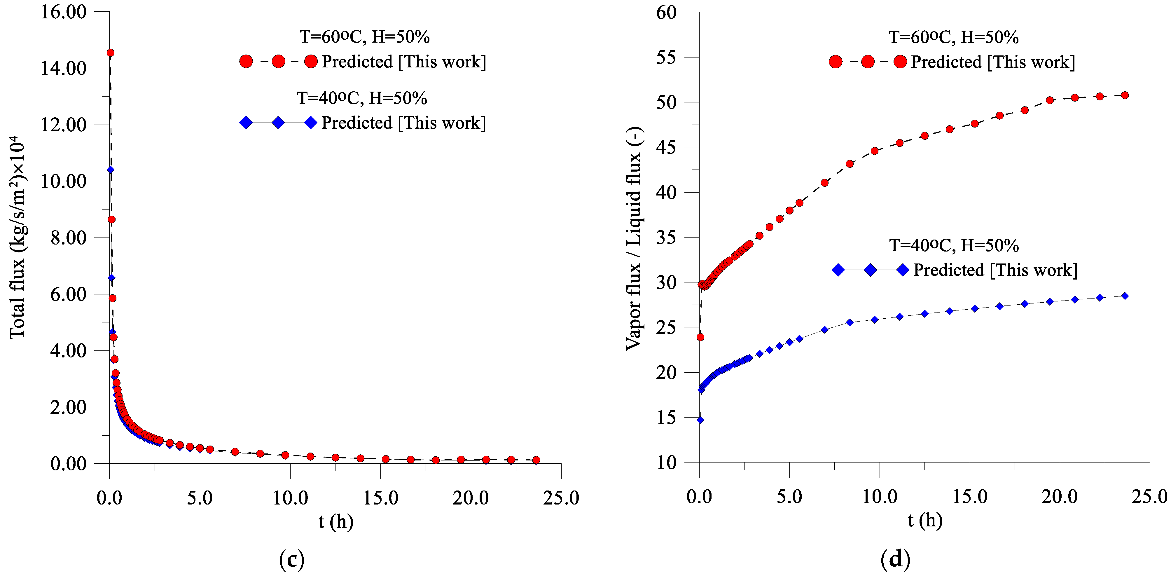
3.2. Fluxes of Liquid, Water Vapor, and Heat

Figure 6a–d present the behavior of the liquid, vapor, and liquid plus vapor fluxes and the relationship between the vapor and liquid fluxes on the surface of the lentil grain obtained during the drying process.

It is possible to observe, in Figure 6, that the liquid and vapor fluxes decrease rapidly in the first two hours of the drying process, tending to zero (hygroscopic equilibrium condition), for long process times (t > 20 h.) It is also noted that in the initial drying times, there are differences between the values of liquid and vapor fluxes, with predominance for the vapor flux, and during the majority of the drying process, the behavior was practically the same, at both the drying air temperature. In the beginning, the value of the vapor flux on the surface of the lentil grain is 14.7 times higher than the liquid flux for T = 40 °C, and 23.9 times higher than the liquid flux for T = 60 °C, growing with the drying time, especially at T = 60 °C, due to the decrease in moisture content in the lentil grain, which evidences the predominance of moisture removal in the form of water vapor. The results also prove that for materials with low initial moisture content, the predominance is for the vapor flux. Probably, for hygroscopic materials with high initial moisture content, such as fruits and vegetables, the relationship between vapor and liquid fluxes in the initial drying times is much lower, tending to increase with the decrease in moisture content throughout the drying process. It is important to note that this result could not have been detected when using the theory of liquid diffusion to describe the drying process of lentil grains; this theory assumes that moisture migrates only in the liquid phase inside the material, regardless of the drying temperature.

Figure 7 shows the heat flux on the surface of the lentil grain during the drying process. It is possible to observe that, during the drying time, the heat flux decreased significantly up to 2 h of drying; after this time, the heat flux decays more slowly, tending to remain constant until the end of the drying process (thermal equilibrium). This heat is used both to heat the grain and water in the liquid phase up to the saturation temperature (sensitive heat) and to evaporate, at saturation temperature, the moisture of the grain that reaches the surface (latent heat). For both the air temperature, heat flux presented almost the same transient behavior. However, at 200 s, heat flux reached the value 3996.14 W/m² at T = 40 °C, and 5409.48 W/m² at T = 60 °C.

3.3. Distribution of Moisture Content and Temperature Inside the Lentil Grain

Figure 8 shows the distributions of moisture content inside the lentil grain in six drying process times (1000, 5000, 10,000, 20,000, 40,000, and 85,000 s). In these figures, the moisture contents inside the solid are represented by the iso-moisture lines. Analyzing these figures, it is possible to observe that the moisture (in the forms of liquid and vapor) migrates from the center to the surface of the lentil grain, and the higher gradients are close to the surface of the grain, especially in the region located near the focal point (y = L₂).

The temperature distribution inside the lentil grain is presented in Figure 9, at times 1000, 5000, 10,000, 20,000, 40,000 and 85,000 s. The constant temperature lines (isotherms) showed that the heating is faster on the surface of the solid, and this heating process occurs from the surface to the center of the body, unlike that of the moisture content. However, unlike what has been verified for moisture content, the temperature distribution inside the lentil grain is practically uniform at any drying time, a typical condition of low convective effects.

From the physical point of view, lower hydric and thermal gradients inside the grain are desirable, since it significantly reduces the damage caused by hydric and thermal stresses, which leads to an increase in the quality of the post-drying product.

3.4. Transport Coefficients Evaluation (k_l, k_v, and h_m)

Table 2. Comparison between the liquid and vapor conductivity and residual error.

Case		a1 (----)	a2 (----)	hm (m/s)	hc (W/m2K)	ERMQ (kg/kg)2	${\overline{\mathbf{S}}}^2(\mathbf{kg}/\mathbf{kg}{)}^2$	R2
T (°C)	H (%)
40	50	2.33 × 104	25.07 × 102	6.20 × 10−6	37.31	0.413 × 103	0.61 × 105	0.996
60	50	1.43 × 104	10.74 × 102	12.80 × 10−6	37.81	1.374 × 103	2.02 × 105	0.991

presents the values of parameters a₁ e a₂ that appear in the transport coefficients (k_v and k_l), the convective mass and heat transfer coefficients (h_m and h_c), the relative error (ERMQ), variance (${\overline{\mathrm{S}}}^2$) and the coefficient of correlation (R²), respectively, determined after the nonlinear regression process. It is possible to observe that the proposed model presented a suitable fit due to the small discrepancy presented between the experimental and numerical data (lower values of ERMQ and ${\overline{\mathrm{S}}}^2$) and a high value of the correlation coefficient.

Applying the coefficients a₁ and a₂ into Equations (44) and (45), respectively, it is possible to observe that the values of liquid and vapor conductivity have inverse behavior during the drying process. While the liquid conductivity decreases during drying, the vapor conductivity increases with the decrease in the moisture content, reaching a maximum vapor conductivity value of 2.35 × 10⁻⁵ m²/s at 40 °C and 1.13 × 10⁻⁵ m²/s at 60 °C. According to Fortes [22], the liquid conductivity increases with moisture content at a given temperature, and, during this increase, there should occur, simultaneously, molecular diffusion of the liquid and vapor, capillary flow, and filtration. For low moisture content values, the migration mechanisms will consist of vaporization-condensation processes. The same author also observed that the vapor conductivity presents a maximum value at low moisture content due to the liquid discontinuity and, consequently, the emptying of pores and capillaries.

Melo et al. [29] obtained, for the same constants, the following values of a₁ = 2.00 × 10⁴ and a₂ = 22.66 × 10², considering the drying process of lentils under the drying conditions T = 40 °C and H = 50%. However, the authors considered an equilibrium boundary condition on the solid surface, which evidences the dependence of these parameters with the boundary condition specified at the surface of the physical domain.

About the fitting process, it is important to notice that the values of the estimated parameters a₁, a_2, and h_m are strongly dependent on the considerations and boundary conditions adopted in the model. For example, relationships between the values of the parameter a₁ obtained when considering convective boundary conditions at the surface of the lentil grain and that considering equilibrium condition is around 1.165 for T = 40 °C.

4. Conclusions

In this research, heat and mass transfer in a porous body with a non-conventional shape was studied. For that, a new and advanced mathematical formulation and its numerical solution (finite volumes) were proposed. From the analysis of the results obtained with the numerical simulation of drying in porous bodies with oblate spheroidal geometry (lentil grain), it is possible to conclude:

(a)

The mathematical model proposed to predict transient diffusion in oblate spheroidal solids, and its numerical solution using the finite-volumes method with the convective condition on the surface was adequate since the predicted values of the average moisture content of the lentil grain along the process presented low deviation and variance when compared with the data of average moisture content obtained experimentally;

(b)

Inside the lentil grain, the dominant mass transfer mechanism is the vapor flux, on the surface of the solid, with a vapor flux/liquid flux ratio greater than 14.7 for T = 40 °C, and greater than 23.9 for T = 60 °C, growing with the drying time, especially at T = 60 °C;

(c)

The areas of lentil grain more susceptible to cracks are located on the surface and around the focal point due to the existence of higher thermal and hydric stresses originated by higher moisture and temperature gradients;

(d)

The liquid conductivity increases with the increase in the moisture content and decreases with the increase in temperature, while the vapor conductivity increases with the decrease in the moisture content and decreases with the increase in temperature due to the behavior of the saturation pressure in the pore inside the porous material.

References

1. Silva, W.P.; Silva, C.D.P.S.; Lima, A.G.B. Uncertainty in the determination of equilibrium moisture content of agricultural products. Rev. Bras. Prod. Agroind. Gd. Espec. 2005, 7, 159–164. (In Portuguese) [Google Scholar]
2. Park, K.J.; Antonio, G.C.; Oliveira, R.A.; Park, K.J.B. Process selection and drying equipments. In Brazilian Congress of Agricultural Engineering; 2006; Volume 35. SBEA/UFCG, Jaboticabal, Brazil (In Portuguese) [Google Scholar]
3. Fellows, P.J. Food Processing Technology: Principles and Practice; CRC Press: Boca Raton, FL, USA, 2009; ISBN 1845696344. [Google Scholar]
4. Park, K.J.; Yado, M.K.M.; Brod, F.P.R. Drying studies of sliced pear bartlett (Pyrus sp.) sliced. Food Sci. Technol. 2001, 21, 288–292. (In Portuguese) [Google Scholar] [CrossRef] [Green Version]
5. Tang, J.; Sokhansanj, S. Moisture diffusivity in laird lentil seed components. Trans. ASAE 1993, 36, 1791–1798. [Google Scholar] [CrossRef]
6. Tang, J.; Sokhansanj, S. Geometric changes in lentil seeds caused by drying. J. Agric. Eng. Res. 1993, 56, 313–326. [Google Scholar] [CrossRef]
7. Wang, J.; Mujumdar, A.S.; Mu, W.; Feng, J.; Zhang, X.; Zhang, Q.; Fang, X.-M.; Gao, Z.-J.; Xiao, H.-W. Grape Drying: Current Status and Future Trends. In Grape and Wine Biotechnology; Morata, A., Loira, I., Eds.; IntechOpen: London, UK, 2016. [Google Scholar] [CrossRef] [Green Version]
8. Hatamipour, M.S.; Mowla, D. Shrinkage of carrots during drying in an inert medium fluidized bed. J. Food Eng. 2002, 55, 247–252. [Google Scholar] [CrossRef]
9. Karim, M.A.; Hawlader, M.N.A. Drying characteristics of banana: Theoretical modelling and experimental validation. J. Food Eng. 2005, 70, 35–45. [Google Scholar] [CrossRef]
10. Li, C.; Li, B.; Huang, J.; Li, C. Energy and exergy analyses of a combined infrared radiation-counterflow circulation (IRCC) corn dryer. Appl. Sci. 2020, 10, 6289. [Google Scholar] [CrossRef]
11. Carvalho, E.R.; Francischini, V.M.; Avelar, S.A.G.; Costa, J.C. Temperatures and periods of drying delay and quality of corn seeds harvested on the ears. J. Seed Sci. 2019, 41, 336–343. [Google Scholar] [CrossRef]
12. Arora, S.; Bharti, S.; Sehgal, V.K. Convective drying kinetics of red chillies. Dry. Technol. 2006, 24, 189–193. [Google Scholar] [CrossRef]
13. Gonelli, A.L.D.; Corrêa, P.C.; Resende, O.; dos Reis Neto, S.A. Study of moisture diffusion in wheat grain drying. Food Sci. Technol. 2007, 27, 135–140. (In Portuguese) [Google Scholar] [CrossRef] [Green Version]
14. Resende, O.; Corrêa, P.C.; Goneli, A.L.D.; Ribeiro, D.M. Physical properties of edible bean during drying: Determination and modelling. Ciência Agrotecnologia 2008, 32, 225–230. (In Portuguese) [Google Scholar] [CrossRef] [Green Version]
15. Doymaz, İ. Convective drying kinetics of strawberry. Chem. Eng. Process. Process. Intensif. 2008, 47, 914–919. [Google Scholar] [CrossRef]
16. Kajiyama, T.; Park, K.J. Influence of feed initial moisture content on spray drying time. Rev. Bras. Prod. Agroind. 2008, 10, 1–8. (In Portuguese) [Google Scholar]
17. Almeida, D.P.; Resende, O.; Costa, L.M.; Mendes, U.C.; de Fátima Sales, J. Drying kinetics of adzuki bean (Vigna angularis). Glob. Sci. Technol. 2009, 2, 72–83. (In Portuguese) [Google Scholar]
18. Lima, W.M.P.B.; Lima, E.S.; Lima, A.R.C.; Oliveira Neto, G.L.; Oliveira, N.G.N.; Farias Neto, S.R.; Lima, A.G.B. Applying phenomenological lumped models in drying process of hollow ceramic materials. Defect Diffus. Forum 2020, 400, 135–145. [Google Scholar] [CrossRef]
19. Fortes, M.; Okos, M.R. A non-equilibrium thermodynamics approach to transport phenomena in capillary porous media. Trans. ASAE 1981, 24, 756–760. [Google Scholar] [CrossRef]
20. Luikov, A.V. Heat and Mass Transfer in Capillary-Porous Bodies; Pergamon Press: New York, NY, USA, 1966; ISBN 0080108326. [Google Scholar]
21. Luikov, A.V. Systems of differential equations of heat and mass transfer in capillary-porous bodies. Int. J. Heat Mass Transf. 1975, 18, 1–14. [Google Scholar] [CrossRef]
22. Fortes, M. A Non-Equilibrium Thermodynamics Approach to Transport Phenomena in Capillary Porous Media with Special Reference to Drying of Grains and Foods. Ph.D. Thesis, Perdue University, West Lafayette, IN, USA, 1978. [Google Scholar]
23. Fortes, M.; Okos, M.R. Drying theories: Their bases and limitations as applied to foods and grains. In Advances in Drying; Hemisphere Publishing Corporation: Washington, DC, USA, 1980; Volume 1, pp. 119–154. [Google Scholar]
24. de Oliveira, V.A.B.; Lima, A.G.B. de Drying of wheat based on the non-equilibrium thermodynamics: A numerical study. Dry. Technol. 2009, 27, 306–313. [Google Scholar] [CrossRef]
25. Oliveira, V.A.B.; Lima, W.; Farias Neto, S.R.; Lima, A.G.B. Heat and mass diffusion and shrinkage in prolate spheroidal bodies based on non-equilibrium thermodynamics: A numerical investigation. J. Porous Media 2011, 14, 593–605. [Google Scholar] [CrossRef]
26. Oliveira, V.A.B.; Lima, A.G.B.; Silva, C.J. Drying of wheat: A numerical study based on the non-equilibrium thermodynamics. Int. J. Food Eng. 2012, 8, 8. [Google Scholar] [CrossRef]
27. Carmo, J.E.F.; Lima, A.G.B. Mass transfer inside oblate spheroidal solids: Modelling and simulation. Braz. J. Chem. Eng. 2008, 25, 19–26. [Google Scholar] [CrossRef]
28. Melo, J.C.S.; Lima, A.G.B.; Pereira Silva, W.; Lima, W.M.P. Heat and Mass Transfer during Drying of Lentil Based on the Non-Equilibrium Thermodynamics: A Numerical Study. Defect Diffus. Forum 2015, 365, 285–290. [Google Scholar] [CrossRef]
29. Melo, J.C.S.; Gomez, R.S.; Silva, J.B., Jr.; Queiroga, A.X.; Dantas, R.L.; Lima, A.G.B.; Silva, W.P. Drying of Oblate Spheroidal Solids via Model Based on the Non-Equilibrium Thermodynamics. Diffus. Found. 2020, 25, 83–98. [Google Scholar] [CrossRef]
30. Magnus, W.; Oberhettinger, F.; Soni, R.P. Formulas and Theorems for the Special Functions of Mathematical Physics; Springer: Berlim, Germany, 1966; Volume 52, ISBN 3662117614. [Google Scholar]
31. Maliska, C.R. Heat Transfer and Computational Fluid Mechanics; Grupo Gen-LTC: Rio de Janeiro, Brazil, 2017; ISBN 8521633351. (In Portuguese) [Google Scholar]
32. Whitaker, S. Heat and mass transfer in granular porous media. Adv. Dry. 1980, 1, 23–61. [Google Scholar]
33. Patankar, S. Numerical Heat Transfer and Fluid Flow; CRC Press: Boca Raton, FL, USA, 1980; ISBN 1482234211. [Google Scholar]
34. Fortes, M.; Okos, M.R.; Barrett, J.R., Jr. Heat and mass transfer analysis of intra-kernel wheat drying and rewetting. J. Agric. Eng. Res. 1981, 26, 109–125. [Google Scholar] [CrossRef]
35. Menkov, N.D. Moisture sorption isotherms of lentil seeds at several temperatures. J. Food Eng. 2000, 44, 205–211. [Google Scholar] [CrossRef]
36. Tang, J.; Sokhansanj, S. A model for thin-layer drying of lentils. Dry. Technol. 1994, 12, 849–867. [Google Scholar] [CrossRef]
37. Figliola, R.S.; Beasley, D.E. Theory and Design for Mechanical Measurements; John Wiley & Sons: New York, NY, USA, 2020; ISBN 1119723450. [Google Scholar]
38. Silva, W.P.; Silva, C.M.D.P.S. LAB Fit Curve Fitting Software (Nonlinear Regression and Treatment of Data Program) V. 7.2.46 2009. Available online: www.labfit.net (accessed on 17 April 2021). (In Portuguese).
39. Tang, J.; Sokhansanj, S.; Yannacopoulos, S.; Kasap, S.O. Specific heat capacity of lentil seeds by differential scanning calorimetry. Trans. ASAE 1991, 34, 517–522. [Google Scholar] [CrossRef]
40. Cengel, Y. Heat and Mass Transfer: Fundamentals and Applications; McGraw-Hill: New York, NY, USA, 2014; ISBN 0077654765. [Google Scholar]
Figure 1. Features of an oblate spheroidal body.
Energies 14 03405 g001
Figure 2. Continuous surface subdivided into nodal points. (a) Identification of the control volume and (b) geometric parameters of the control volume in the oblate spheroidal coordinates system.
Energies 14 03405 g002
Figure 3. Sketch of the control volume on the surface of the solid and its characteristic dimensions.
Energies 14 03405 g003
Figure 4. Predicted and experimental average moisture contents of lentils during drying at 40 °C and 60 °C and a relative humidity of 50%.
Energies 14 03405 g004
Figure 5. Average temperature of lentil grain over time during drying at 40 °C and 60 °C and a relative humidity of 50%.
Energies 14 03405 g005
Figure 6. (a) Liquid flux, (b) vapor flux, (c) total flux, and (d) relationship between the vapor flux and the liquid flux, on the surface of the lentil grain for drying at 40 °C and a relative humidity of 50%.
Energies 14 03405 g006aEnergies 14 03405 g006b
Figure 7. Heat flux on the surface of lentil grain for drying at 40 °C and a relative humidity of 50%.
Energies 14 03405 g007
Figure 8. Distribution of moisture content inside lentil grain at different process moments, for drying at 40 °C and a relative humidity of 50%.
Energies 14 03405 g008
Figure 9. Temperature distribution inside the lentil grain at different process moments, for drying at 40 °C and a relative humidity of 50%.
Energies 14 03405 g009