Article

Influence of Errors in Known Constants and Boundary Conditions on Solutions of Inverse Heat Conduction Problem

Department of Mechanical System Design Engineering, Seoul National University of Science and Technology, Seoul 01811, Korea
Energies 2021, 14(11), 3313; https://doi.org/10.3390/en14113313
Submission received: 30 March 2021 / Revised: 28 May 2021 / Accepted: 1 June 2021 / Published: 4 June 2021
(This article belongs to the Special Issue Modelling of Thermal and Energy Systems)

Abstract

:
This work examines the effects of the known boundary conditions on the accuracy of the solution in one-dimensional inverse heat conduction problems. The failures in many applications of these problems are attributed to inaccuracy of the specified constants and boundary conditions. Since the boundary conditions and material properties in most thermal problems are imposed with uncertainty, the effects of their inaccuracy should be understood prior to the inverse analyses. The deviation from the exact solution has been examined for each case according to the errors in material properties, boundary location, and known boundary conditions. The results show that the effects of such errors are dramatic. Based on these results, the applicability and limitations of the inverse heat conduction analyses have been evaluated and discussed.

1. Introduction

The inverse heat conduction problem (IHCP) has become one of the most solved problems in heat transfer [1]. Since Beck [2] and Alifanov [3] established the sequential method and the gradient method, respectively, there have been a large number of applications using those methods. In particular, many works have tried to retrieve the boundary conditions from the experimental data [1]. The method has been applied to various processes, including casting [4,5], composite processing [6], and welding [7,8].
However, the matter related to known boundary conditions is one of the least studied parts of IHCP, despite the long history of the related studies. The reason is not because it is unimportant, but because it is simply assumed known in IHCP while defining the problem. However, in reality, there is no such boundary condition (BC) that is accurately known without measurement, even though correlations are employed. For example, consider a surface subject to forced air convection with a developing laminar thermal boundary layer. Simply by measuring temperature and velocity of free stream, it might be possible to find a suitable correlation and determine the heat transfer coefficient (HTC). However, the uncertainty of HTC is unlikely to be assessed since the heat transfer that needs inverse analysis would not take place somewhere like a wind tunnel. Thus, it requires a lot of cautions to specify the boundary condition, which is presumed to be known. Sometimes, the adiabatic condition is imposed on an insulated boundary. However, there is no such boundary in engineering applications that prevents heat flow perfectly.
Moreover, the material properties, such as the thermal conductivity and the thermal diffusivity, can include inaccuracies. The material tests, which are always challenges to many thermal engineers, can induce errors. Or, sometimes, the test is impossible and the IHCP should be solved with the material properties in the literature. Another kind of error comes from fabrication, installation, instrumentation and, dimensional measurement. The position of thermocouples and boundaries can be inaccurate. These inaccuracies can undermine all the elaborations to make the IHCP solution improved. Although steady problems are also of interest in some cases [9,10], most IHCPs are on transient problems. Thus, a lot of efforts have been made to overcome numerical instability from the time marching. Before trying to employ multidimensional [7,8,11,12] or nonlinear methods [13,14,15], the solution characteristics with the one-dimensional linear IHCP should be checked first [3].
The purpose of this work is quite straightforward. It is to show the risks involved in solving IHCP when incorrect values are engaged in the setup. This work simply follows the established procedures of the gradient method with the Tikhonov regularization based on the adjoint formulation [16,17]. It is a whole domain method that provides the search direction by solving the adjoint differential equation [3]. The whole procedure to the IHCP solution by this method is fairly involving, but already well described in several literatures, and its performance has been proven by many researchers [1,3,18,19]. A rigorous error analysis of the gradient method can be found in [20].
Since this work is neither about new methodologies nor about new applications, the method will be described in the simplest possible way. In this work, a general setup for the one–dimensional linear IHCP with constant material properties is presented. Since the heat flux boundary condition in this work is not parameterized, the number of unknowns is equal to the number of time steps. Note that the boundary condition can be parameterized using a priori information to reduce the number of unknowns [1,3,21]
Then, its numerical implementation of the setup will be realized in Microsoft Excel with a VBA code, which will be publicly open to allow others to evaluate the risk of incorrect constants. Moreover, as it is currently impossible to find an open computer code for the IHCP, this code can be a useful reference for engineering and developments [22].
This work has investigated the effects caused by inaccurate specification of material properties, known BC, and positions of the sensor and boundary. Because the methods dealing with noisy measurements have been thoroughly investigated, this work has tried to minimize the contents relevant to that to emphasize the bias by the incorrect specifications of the BC and constants. The effects of each incorrectly specified value, presumed known prior to the analysis, have been tested, examined, and discussed.

2. Inverse Methods

2.1. Inverse Problem and Equations

Consider an inverse heat conduction problem as shown in Figure 1. This is a general setup for a linear IHCP with constant properties that features multiple sensors and typical three kinds of known boundary conditions. The unknown heat flux condition, q0, will be imposed at x0, while one of temperature (Dirichlet) T1, heat flux (Neumann) q1, or heat transfer coefficient (Robin) h, and the ambient temperature T , can be specified at x1. A temperature history at x = x0, T 0 t , is calculated together with q0. The inverse problem seeks the unknown heat flux, q 0 ( t ) , with the temperature measurements, Y j t , at plural sensor locations, x = s j , for j = 1 to Ns. Note that it is straightforward to retrieve the HTC, h 0 ( t ) , when the ambient temperature, T , 0 , is known on Ω 0 by h 0 ( t ) = q 0 ( t ) / [ T , 0 T 0 ( t ) ] .
When the measurement data are acquired for a time interval between t 0 = 0 and t f , the residual, J q 0 , is expressed as:
J q 0 = t 0 t f j = 1 N s T s j , t ; q 0 Y j t 2 d t
When a zero-th order regularization term is added to the above expression, we have:
J R 0 q 0 = J q 0 + R 0 t = t 0 t f q 0 q r 0 2 d t
where R 0 is the regularization parameter and q r 0 is the reference heat flux.
Given a constant standard deviation, σ, of measurement data gives:
T s j , t ; q 0 Y j t σ
Thus, the IHCP has to determine a solution that meets:
J q 0 N s σ 2 t f t 0
To update the temperature field T x , t ; q 0 , it is necessary to solve the direct problem shown in Figure 1, which is the following one-dimensional heat conduction equation for a homogeneous solid medium between x0 = 0 and x1:
T t = α 2 T x 2   in   Ω   for   t 0 < t t f
where α is the thermal diffusivity.
The initial condition is:
T ( x , t 0 ) = T i x   in   Ω
The bottom side of the boundary is subject to a Neumann condition:
k T x x 0 , t = q 0 ( t )   on   Ω 0
where k is thermal conductivity and q 0 ( t ) is the unknown heat flux that should be determined from the solution of the IHCP. On the other hand, one of the following conditions can be imposed on Ω 1 :
T x 1 , t = T 1 t
k T x x 1 , t = q 1 t
k T x x 1 , t = h T x 1 , t T
where T 1 t , q 1 t , h, and T should be known prior to imposition.
To achieve a solution that satisfies Equation (3), an optimization procedure is essential. In this work, the gradient for the optimization is obtained by the adjoint formulation. Refer to [3,19] for detailed derivations of the adjoint problem. The gradient is evaluated from a solution of the adjoint problem, λ ( x , t ) . The gradient is of the form:
J R 0 q 0 = λ ( x , t ) + 2 R 0 t = t 0 t f q 0 q r 0 d t
where λ ( x , t ) is obtained by solving the following adjoint problem [1,3]:
λ t = α 2 λ x 2 + 2 j = 1 N s δ x s j T s j , t ; q 0 Y j t   in   Ω ,   t 0 < t t f
with a final time condition of:
λ ( x , t f ) = 0
The corresponding boundary condition on x = x 0 is:
k λ x x 0 , t = 0   on   Ω 0
The same kind of boundary condition should be imposed on Ω 1 according to the boundary condition of the direct problem.
k λ x x 1 , t = 0
k λ x x 1 , t = 0
k λ x L , t = h 1 λ L , t
Basically, since the gradient can be determined by solving Equation (6a), any gradient-based method, which takes its objective as Equation (1), can seek an IHCP solution by updating the temperature field by solving Equation (4a). This work employs the conjugate direction method (CGM), as in many previous works with the adjoint formalism. In the r-th iteration of the optimization procedure, the new heat flux value is updated by:
q 0 r + 1 = q 0 r + β ϕ P r
where ϕ is the relaxation parameter and β is the step size. Here, the search direction in the CGM is determined by:
P r = J r + γ P r 1
where the conjugate coefficient is determined by:
γ r = t = t 0 t f J r 2 d t t = t 0 t f J r 1 2 d t
Once a search direction, P r , is determined, it is required to find the step length, β, that makes J q 0 r β P r minimum. The step length, β, can be determined by:
β = t = t 0 t f j = 1 N s Δ T s j , t T s j , t ; q 0 Y j t d t t = t 0 t f j = 1 N s Δ T s j , t 2 d t
where the increment of temperature is Δ T ( x , t ) T x , t ; q 0 + Δ q 0 T x , t ; q 0 , when the unknown heat flux is increased by an amount of Δ q 0 ( t ) = P . Fortunately, Δ T ( x , t ) can be solved by solving the following sensitivity problem:
Δ T t = α 2 Δ T x 2   in   Ω ,   t 0 < t t f
with a final time condition of:
Δ T ( x , t 0 ) = 0
The corresponding boundary condition on x = x 0 is:
k Δ T x x 0 , t = Δ q 0 ( t )
One of the following conditions is imposed on Ω 1 corresponding to the boundary condition of the direct problem:
Δ T x 1 , t = 0
k Δ T x x 1 , t = 0
k Δ T x x 1 , t = h Δ T x 1 , t
These are all the mathematical expressions necessary for solving the linear IHCP shown in Figure 1.

2.2. Discretization

A uniform interval of data sampling, ∆t, and a mesh with uniform spacing, ∆x are set for simplicity. Thus, the discrete time is:
t k = k Δ t + t 0   for   k = 0   to   N t
The final time is given as t f = N t Δ t + t 0 and the numerical time step is set equal to the sampling interval. Similarly, the spatial domain is discretized between x0 to x1 as:
x i = i Δ x + x 0   for   i = 0   to   N x
All the temperature calculated here is denoted as:
T i k q 0 = T i t k ; q 0 = T x i , t k ; q 0
The measured and calculated temperatures at j-th location are represented as T ¯ j t and Y j t , respectively. The calculated temperature at Tik at xi = sj is represented by T ¯ j k = T s j , t k ; q 0 . Both temperatures should satisfy T ¯ j k q 0 k Y j k σ . In this discretized domain, Equation (1) is written as:
J q 0 = k = 0 N t j = 1 N s T ¯ j k Y j k 2 Δ t
Based on the discretization in [18], the temperature in Equation (4a) can be updated by:
a p T i k + 1 = a p 2 1 θ a 0 T i k + a 0 θ T i + 1 k + 1 + 1 θ T i + 1 k 1 + a 0 θ T i 1 k + 1 + 1 θ T i 1 k 1
where a P = Δ x / Δ t and a 0 = α / Δ x . Moreover, the Crank–Nicolson scheme is adopted by setting for θ = 0.5 . Fortunately, Equation (16) forms a tridiagonal matrix, and the solution can be sought fast by the TDMA (tridiagonal matrix algorithm).

2.3. Implementations

The calculation in this work is conducted as carried out in the previous works [18,19]. The iteration loop for the optimization of Equation (1) is comprised of the following procedure:
Update T x , t ; q 0 with current q 0 by solving Equation (4a).
Calculate the gradient in Equation (5) by solving Equation (6a).
Calculate the update direction by Equation (8) with the conjugate coefficient from Equation (9).
Solve Equation (11a) with setting Δ q 0 in Equation (11c) as the update direction.
Determine the step length by Equation (10).
Update q 0 by Equation (7).
The solution of this IHCP should satisfy Equation (3) by adjusting R0 in Equation (1b). Iteration stoppage is sometimes not accurate enough. Thus, a suitable R0 should be found by trial and error to meet:
σ ε 2 J q 0 N s σ 2 t f t 0 σ + ε 2
where ε is set as σ/100 in this work. As mentioned earlier, the whole procedure is coded in Microsoft Excel using VBA (visual basic for applications) and is available in [22].

3. Results and Discussions

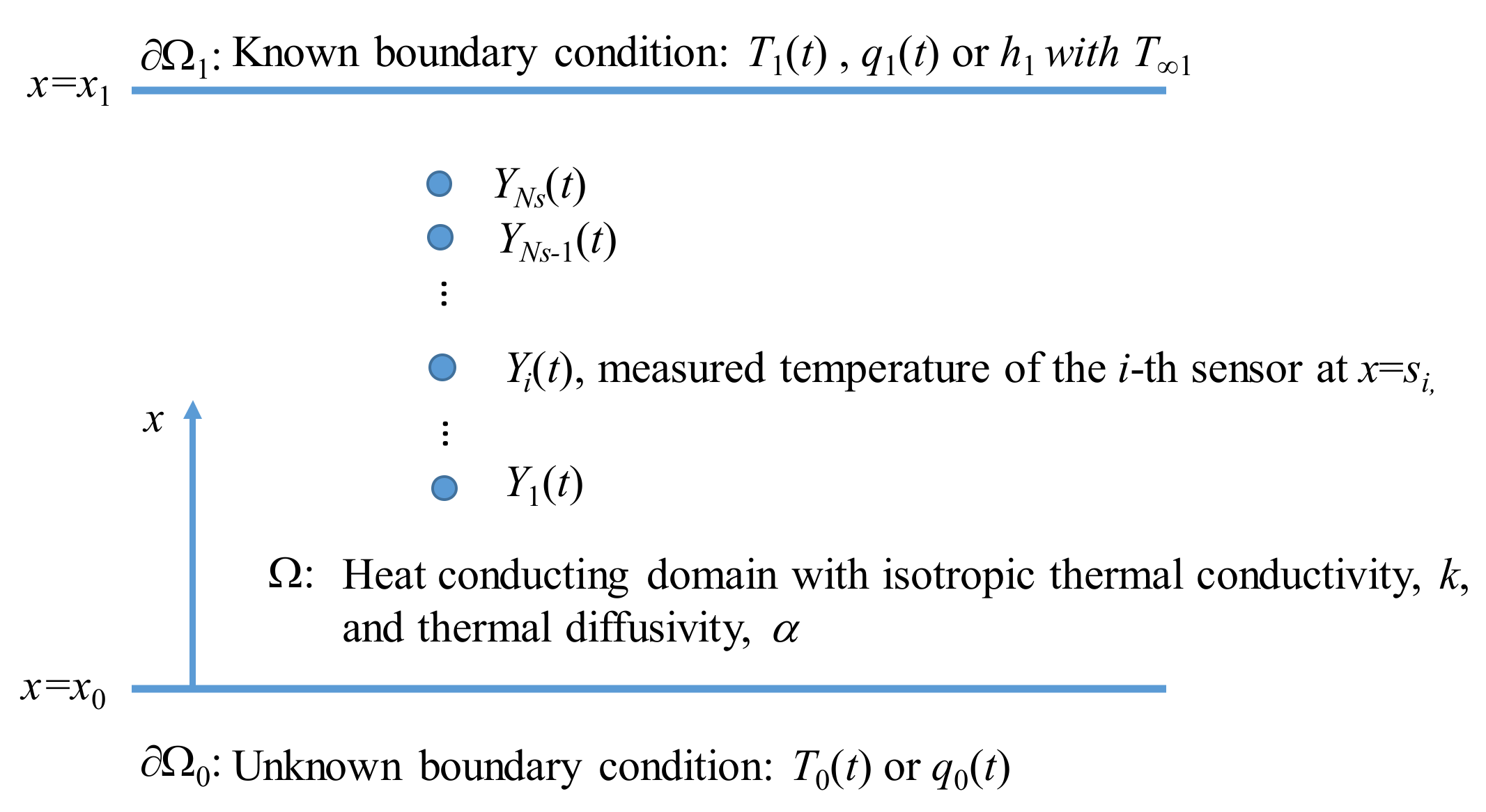
3.1. Basic Results and Sensor Locations

Figure 2 compares the recovered heat fluxes obtained using the errorless measurement data obtained at different sensor locations. The exact heat flux plotted together in the figure is the one that is imposed to obtain the virtual measurement data. The heat flux form to be retrieved is a rectangular form that is usually selected to measure the performance of the inverse estimator, since it has abrupt changes. The default values for the tests are specified in Table 1. The estimation stops by taking σ = 10−5 °C to avoid the possible infinite loop by σ = 0 °C.
All the tried cases in Figure 2 recover the unknown heat flux quite well. showing reduction of the gradients in the rising and the falling edges, along with the distance of the sensor from the surface. The capability of recovering such sharp edges characterizes the deterministic bias of this inverse estimator. The biases shown in Figure 2 are inherent in the solution characteristics and are dependent on the strength of the causal relationship between the BC to be reconstructed and the source of the measurement. As the sensor locations move away from the boundary of the unknown heat flux, the solution becomes inaccurate, showing more deviation near the rising and the falling edges. The biases in Figure 2 change mildly, along with the distances. However, it would be quite severer with engagement of measurement errors.
Figure 3 shows the recovered heat flux, along with the distances for σ = 0.057 °C and Δ T = ± 0.1   ° C . The bias, along with the distance, dramatically changes, as can be seen in the plot. The effect of the measurement errors has been investigated thoroughly, since the inherent resolution loss due to the errors was considered the major source of the solution inaccuracy. However, as aforementioned, the measurement error is not the only source of failure in inverse heat conduction analyses. The sensor location can be incorrectly informed due to several reasons. For example, the drilling hole for a thermocouple can be deeper or shallower, or the sensor can be dislocated unwantedly. Figure 4 shows the estimated heat fluxes when the sensor location is incorrectly known. As the sensor location, s1, is set closer to x0, the estimated heat flux becomes smaller, especially near the rising edge, while the reverse happens as s1 moves away from x0. The error in the sensor location does not seem to cause an oscillation in the solution, but deviation is pronounced near both edges. In the rest of this work, only errorless cases with σ = 0 °C have been treated, to highlight the effects of the incorrect known boundary conditions.

3.2. Material Properties

In the linear IHCPs with constant material properties, the only material property appearing in the governing equation is the thermal diffusivity. The thermal conductivity shows up only in the boundary conditions. With the same thermal conductivity, the thermal diffusivity has been varied to investigate the effects of the incorrect thermal diffusivities. Figure 5 shows the heat flux estimated with incorrect thermal diffusivities. The reduced thermal diffusivity exaggerates the solution at the rising and falling edges, as shown in Figure 5. The increased thermal diffusivity renders the solution underestimated at both edges, but it is severer at the rising edge. Figure 6 shows the temperature on ∂Ω0 estimated with incorrect thermal diffusivities. Similar trends as in Figure 5 are reproduced here. What is interesting here is the trends in Figure 4 are similar to those in Figure 5 and Figure 6. The dislocation of the sensor changes the travel time for the thermal signal from the surface to the sensor, as the thermal diffusivity changes the travel time by t ~ L 2 / α where L is the distance between the sensor location and the bottom boundary.
Figure 7 shows the reconstructed heat fluxes, along with the incorrectly specified thermal conductivity. Because the thermal diffusivity is unchanged, the incorrect imposition only affects the boundary condition. As a result, the reduced thermal conductivity shifts the solution upward, while the increased one moves down the solution, as can be seen in the figure.
The incorrect specification of the thermal properties only happens when the thermal properties cannot be measured. This situation can arise because of various reasons, such as unavailability of material, difficulty of tests, and change of properties in an integrated system. It can be stated that the incorrect thermal diffusivity is riskier than such thermal conductivity, since the thermal diffusivity is directly related to the parabolic nature of the heat equation. The effects of the Fourier number, α Δ t / L 2 , are well described in [1,2,3].

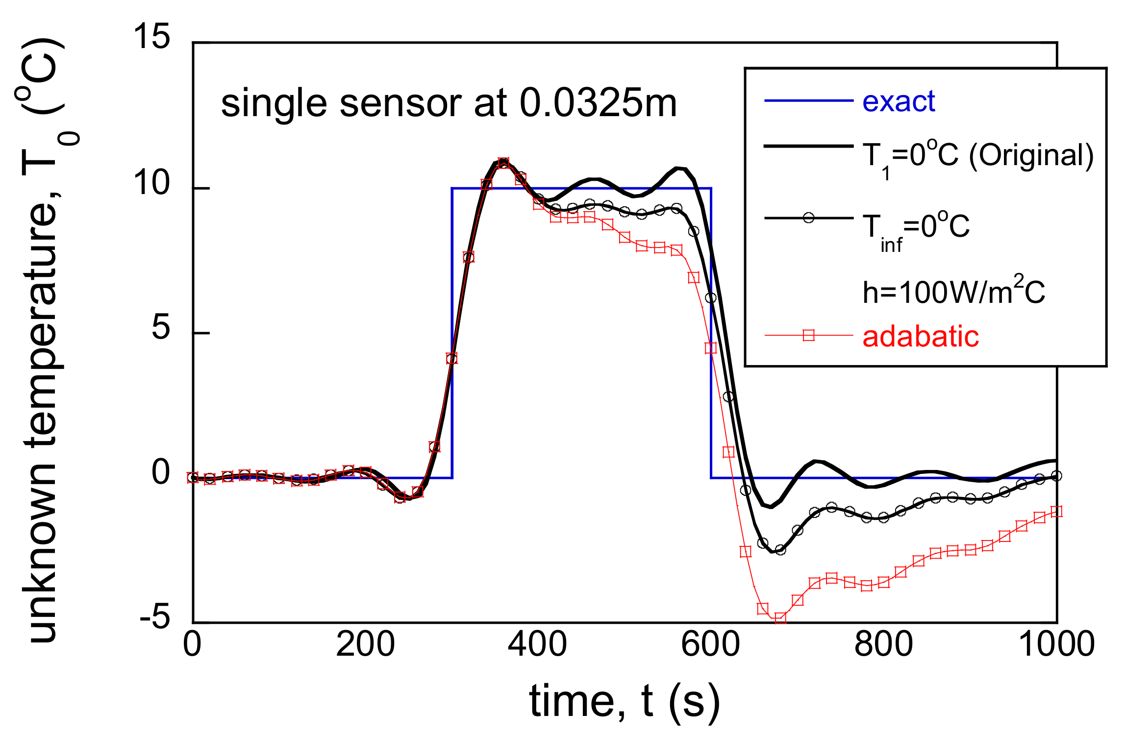
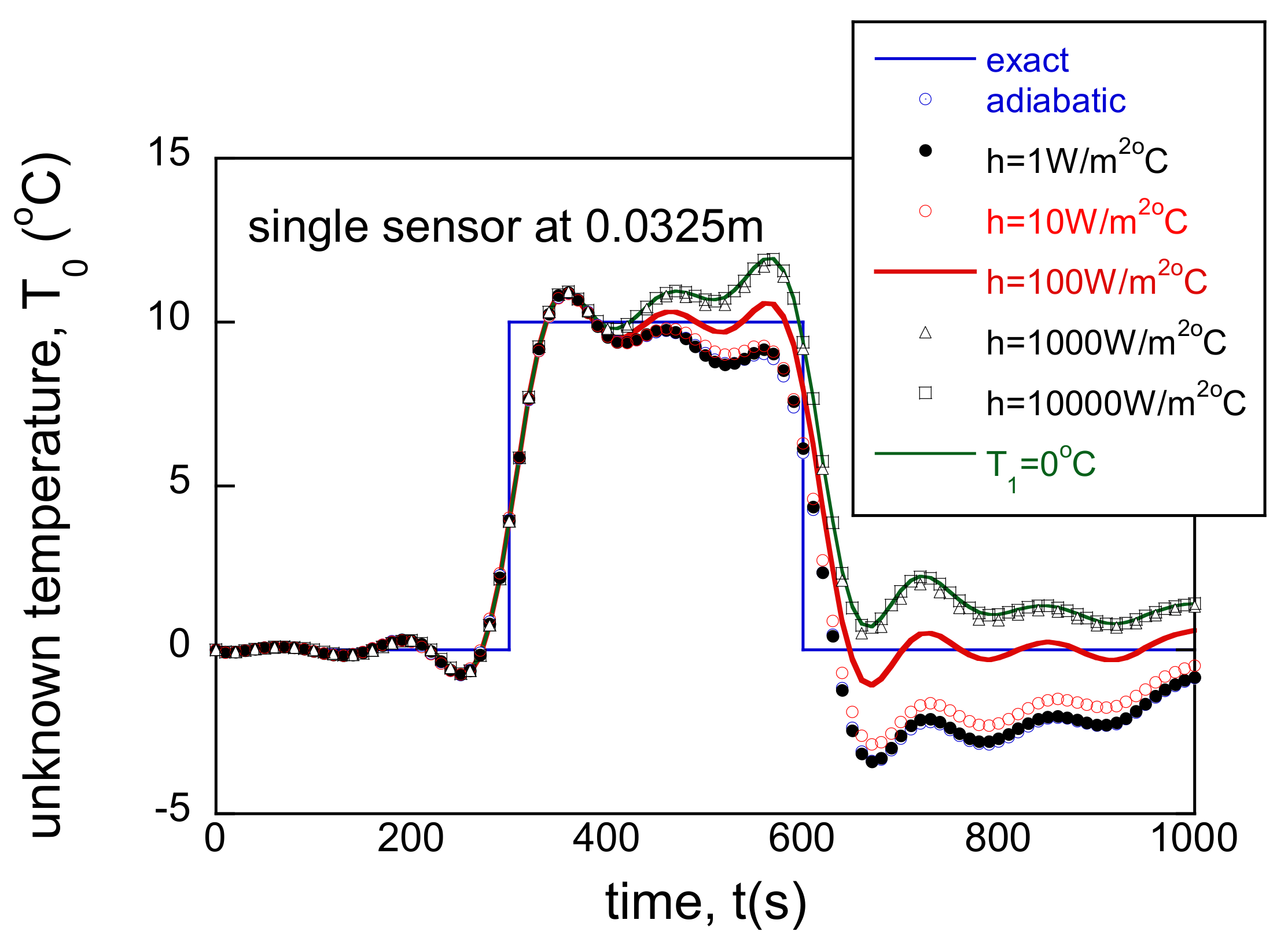
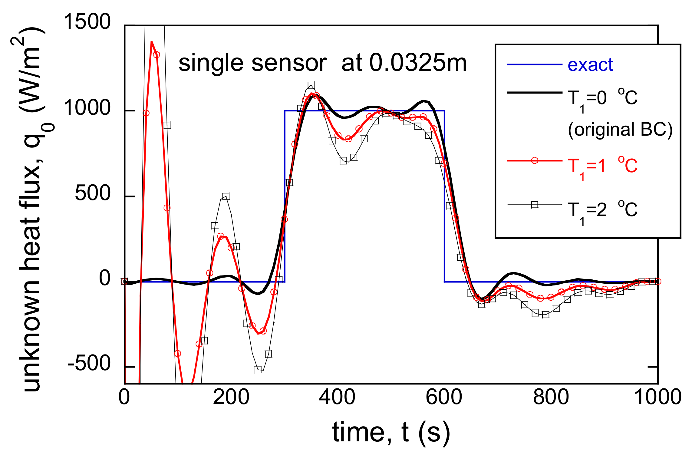
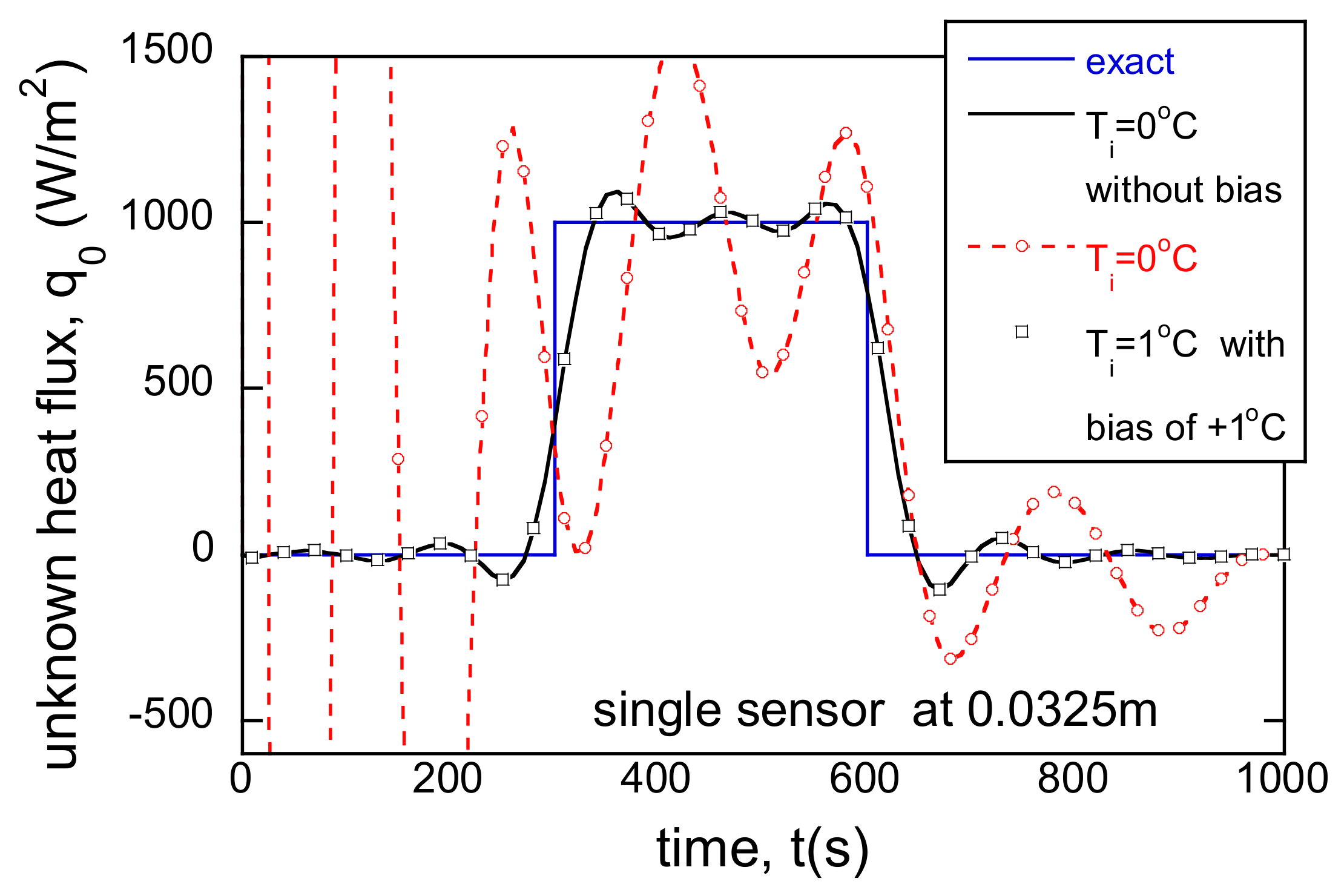
3.3. Incorrect BC and Single Sensor

As an introductory problem of incorrectly specified BC, consider a case where both the correct unknown and known BCs are Dirichlet conditions. As stated previously, it can often be difficult to identify the accurate BC in a real estimation. When a convective BC or an adiabatic condition are specified, the solutions will be changed. Figure 8 shows the estimated heat flux according to the BC specified on ∂Ω1. The three curves move together until 400 s, but they separate after then. Since the initial condition, Ti = 0 °C, before the heat wave by the heat flux on ∂Ω0 does not reach ∂Ω1, the BC does not affect the solution. The altered BC actually changes the heat loss on ∂Ω1. The adiabatic condition causes the largest error, since it blocks all the heat loss. The error is reduced for the case with the convective BC of h = 100 W/m2K and T = 0 °C since it implies the temperature specification with a thermal resistance of 1/h.
Figure 9 shows the measured and the estimated temperatures at the same location for all three cases. Despite the different BCs, the estimated temperatures at the sensor location are almost identical. Thus, this comparison cannot be employed as an indicator for determination of the success of the estimation. The results in Figure 8 and Figure 9 implicate the following: first, wrong specification of the BC does not result in failure of estimation; second, false imposition of the BC causes a strongly biased inverse solution.
Let us examine the effects of the incorrectly imposed HTC on ∂Ω1. Figure 10 compares the estimated inverse solutions obtained by imposing different HTCs when the exact value is 100 W/m2 °C. The increased and decreased HTCs make the solutions near the end of the time deviated. The increased HTC virtually takes more heat from the BC, so that the heat flux on ∂Ω0 is overestimated. The impositions of 1000 W/m2 °C, 10000 W/m2 °C, and T 1 = T give almost the same results, since h = 1000 W/m2 °C means a negligible thermal resistance in this setup. Meanwhile, the reduced HTC decreases heat loss on ∂Ω1 and results in negative heat flux on ∂Ω0.
So far, the cases with T 1 = T i = 0 °C or T = T i = 0 °C have been treated. However, if T T i is imposed when the correct BC requires T = T i , the solution is expected to behave differently. Figure 11 shows the effects of incorrectly specified T when the correct condition is given by T 1 = T i = 0 °C and h = 100 W/m2 °C. The decreased T moves the estimated heat flux upward, while the increased one does the reverse. Moreover, note that the oscillations of the solution in the early time are quite remarkable for T = 2 or 2 °C because of significant discrepancy between T and T i . As time progresses, such an oscillation decays and rather parallel biases are observed. Consequently, the incorrect imposition of T causes a bias proportional to the deviation in T throughout the whole time domain, and oscillations in the early time.
Temperature measurement can be biased by a few causes, such as a shift in the data acquisition system and sensor drift. Moreover, even once the BC is legitimately set, the thermal condition can be altered while acquiring the measurement data. The temperature bias of 1 °C can happen in a usual thermal setup. The unknown heat flux is reconstructed with a Dirichlet BC specified in Figure 12. The bias of 1 °C incurred huge fluctuations in the early time, and relatively small deviation in the later time. The increase of bias to 2 °C magnifies the overall deviations. If T i = 0 °C is set instead, the oscillations in the early time disappear.
It should be investigated how large 1 °C is compared to the overall scale of the measurement data. Let us take look at the measurement data used for reconstruction in Figure 12. As shown in Figure 7, the maximum temperature rise is approximately 4 °C. The biases in the two specified BCs are 25% and 50% of the maximum, respectively. Figure 13 also shows the temperatures estimated with the falsely specified BCs. Despite the large bias in the BC, the estimated temperatures at the sensor location follows the measurement data very well. The only deviation observed in Figure 13 is the upward sway around t = 70 s, despite the large variation in Figure 12. However, the small fluctuation near the early time should not be ignored if observed.
Let us enlarge the estimated temperature in the early time interval. Figure 14 shows the estimated temperature up to 400 s. The oscillation for T1 = 2 °C is very pronounced, although not quite noticeable in Figure 13. This implies that small oscillations in temperature estimation amplify to large ones in inverse solutions. In another aspect, the imposition of a Dirichlet BC requires more cautions than the heat flux or the convection BCs.
Consider cases where the initial condition is incorrectly specified when heat flux has to be estimated. The correct initial condition is Ti = 0 °C in Ω, and the adiabatic condition on ∂Ω1 is specified. Figure 15 shows the effects of altered IC. A small change, such 0.01 °C, leaves a small fluctuation in the very early time, roughly between 1 s and 100 s. When the change is increased to 0.1 °C, the fluctuation in the early time becomes very severe. However, the heat flux estimated for Ti = 0, 0.01 and 0.1 °C coincide with each other at 270 s. The effects of incorrectly specified IC are limited when the error is not large.
Consider a situation where the measured temperature is biased. Figure 16 shows the estimated heat flux using the biased measurement data. The heat flux dramatically oscillates over the entire time domain if it is estimated using the biased data as is. However, if the IC is shifted by the same amount, the erroneous oscillation disappears and the solution is completely corrected. If any biases in the measurement data are found, the correction can be directly imposed on the measurement data or to the IC. It is crucial to avoid biases in measurements of ambient, initial temperatures and Yi.

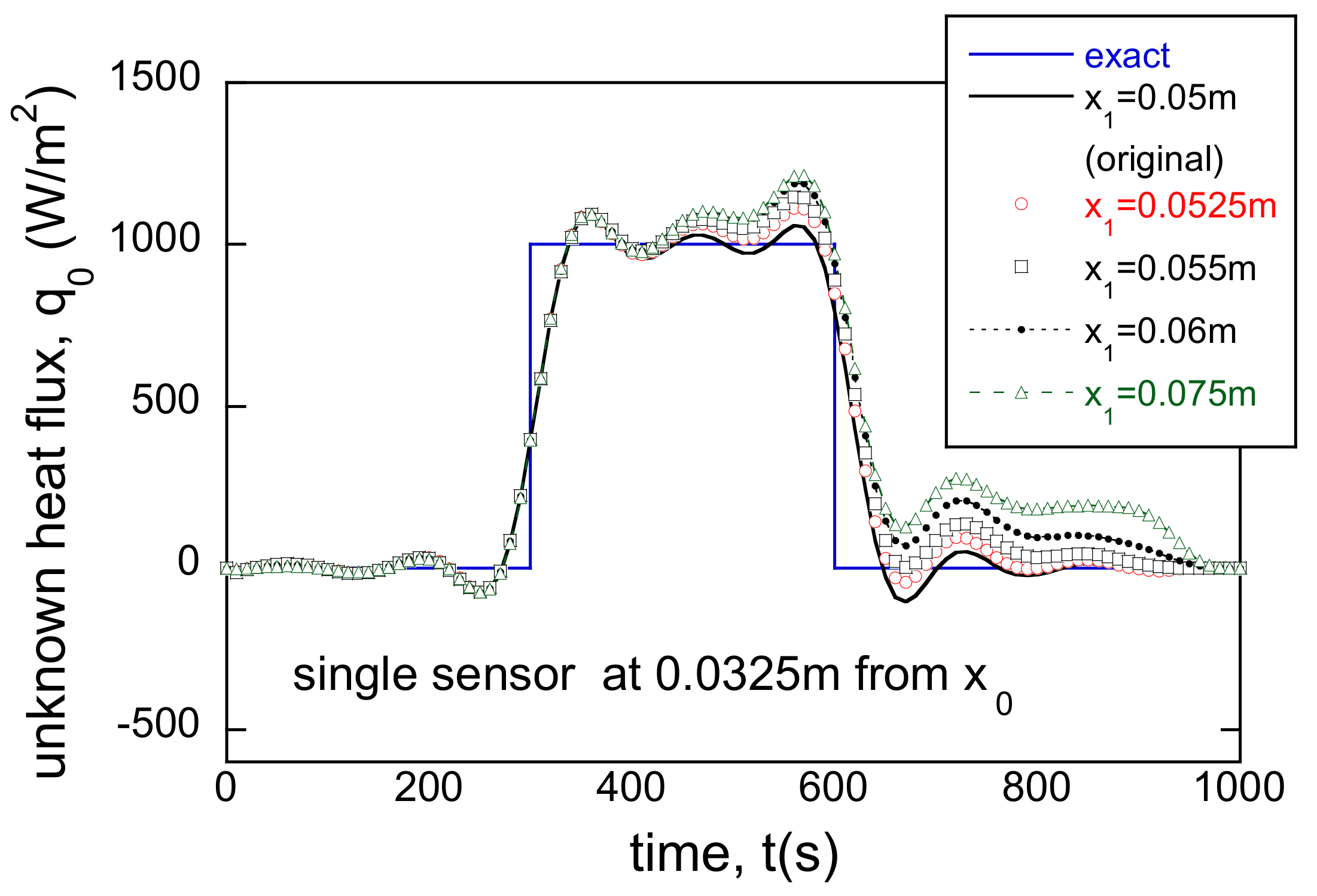
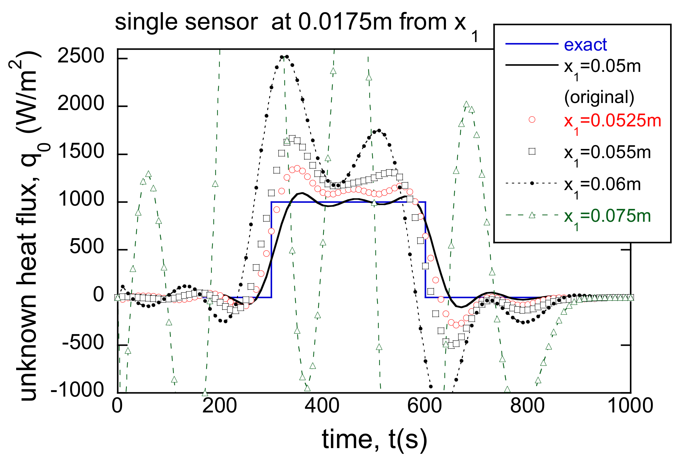
3.4. Incorrect Boundary Locations
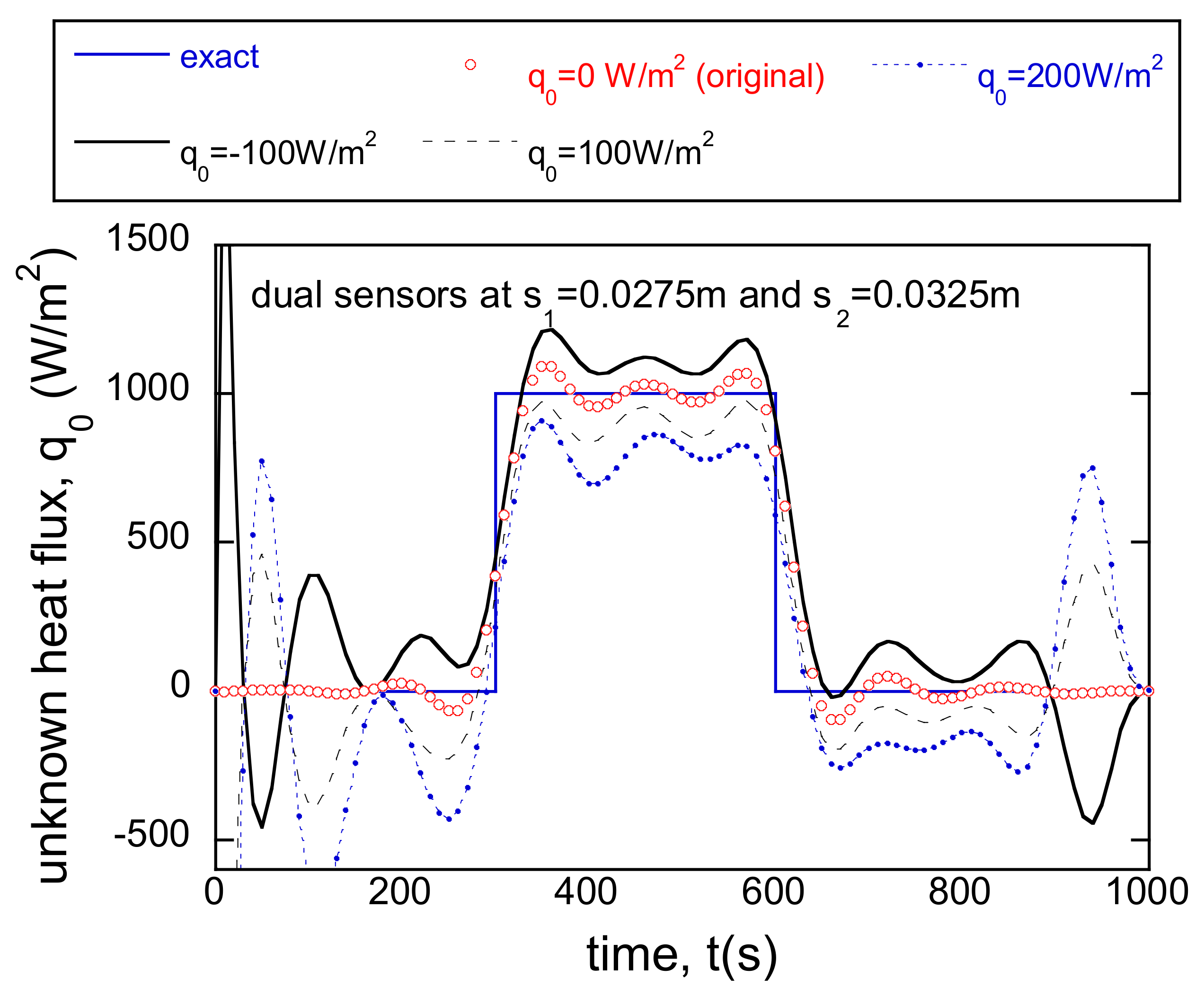
The boundary locations can be incorrectly specified due to some unwanted reasons, such as measurement error, inaccurate fabrication and abrasion. Figure 17 shows the estimated heat fluxes when the distance between the sensor and ∂Ω0 is fixed, while x1 is varied. The heat fluxes follow the original solution up to 450 s. Then, they start to deviate from it as the whole thickness or location of ∂Ω1 increases. The deviation is mild, even with 50% increase of the thickness, since the causal relationship between the heat flux and the sensor is not greatly changed. The increase of the heat flux is necessary to compensate the increased thermal volume.
When the adiabatic condition on ∂Ω1 is replaced by a finite heat flux condition, the solutions would be changed. Figure 18 shows the results when ∂Ω1 is subject to q1 = 100 W/m2. The heat fluxes in the early times fluctuate, but the results are quite similar to those in Figure 17. The fluctuations are due to the cooling rate change by the relationship between the cooled surface and the sensor.
Consider another case where the distance between the boundary of the known BC and sensor is varied. When such distance is incorrect, the error can be large because the distance is engaged in the causal relationship between the information source and the response. When distance between ∂Ω1 and the sensor is fixed as 0.0175 m, the sensor position, s1, is given by x1 − 0.0175 m. Figure 19 shows the heat flux estimated for different x1’s. As the distance increases, the heat flux estimated between 300 s and 600 s increases accordingly. For x1 = 0.06 m, the solution fluctuates significantly, but the rising and falling edges are roughly predicted. However, for x1 = 0.075 m, the estimated heat flux fluctuates so severely that it is almost impossible to predict the original heat flux.

3.5. Dual Sensors

Now, let us discuss the case of the Neumann conditions on ∂Ω1. When the boundary is originally subject to the adiabatic condition, the imposed BC is changed from −100 to +200 W/m2 °C to investigate the effects of the incorrect Neumann conditions. Figure 20 shows the estimated heat flux according to the change of the imposed BC. The positive BC causes a negative initial swing while the negative BC causes a positive one.
One can have an idea that multiple sensors might alleviate such a large swing due to an incorrect BC. The same problems in Figure 20 are solved again with one more sensor at 0.0375 m. The results are presented in Figure 21, but it does not improve the deviations observed in Figure 20. Although it is known that the multiple sensors improve the noise sensitivity and other related characteristics, this matter is put aside in this work. It has to be investigated how the estimated temperatures at the sensor locations follow the temperature measurements. Figure 22 compares the estimated and measured temperatures at s1 = 0.0325 m and s2 = 0.0375 m. Because of the incorrectly specified BC, q0 = −100 W/m2 °C, the estimated temperatures cannot exactly follow the measurement data, unlike the single sensor case in Figure 9. Although the trends in Figure 22 are monotonic, the consistent deviation between the measurement and estimation incurs a dramatic fluctuation in Figure 21 (more specifically the black line for −100 W/m2 °C).
The results in Figure 20 can be improved by adding the extra sensor closer to the surface of the unknown heat flux. Figure 23 shows the heat fluxes estimated using the measurement data read at 0.0275 m and 0.0325 m. It can be stated that the solutions are improved in Figure 23 in comparison with those in Figure 21. However, it cannot be argued that the solutions are improved in comparison with those in the single sensor case shown in Figure 20. These results advise that an additional sensor cannot resolve the issue with maintaining the incorrect BC.
Therefore, an alternative approach is needed. In this one-dimensional IHCP, an extra sensor can eliminate the uncertain BC. Figure 24 illustrates the scheme change by employing the measurement data as the BC. The boundary, ∂Ω1, is moved to s2 and the measurement data, Y2, is imposed as the Dirichlet BC. Figure 25 shows the heat flux estimated by this approach. Using the errorless data, the result reproduces the result by the correct BC. Moreover, the method succeeds even using the noisy measurement data. The filtering of the imposed BC on the altered boundary marginally improves the solution.

4. Conclusions

This work has tested the effects of incorrectly specified constants, such as the material properties, boundary conditions, and sensor locations. The one-dimensional linear inverse heat conduction problem has been described and implemented to perform the tests. The analyses of test results have found several important points. The effects of thermal conductivity errors are proportional to the magnitudes of the errors. and they do not induce severe oscillations. The change in the thermal diffusivity causes the original form of the heat flux to be distorted, but does not incur severe oscillations.
The incorrectly specified boundary condition does not affect the solution until the thermal signal reaches the boundary. Despite the incorrect boundary conditions, the temperature that matches the measurement can be found. It should be emphasized that the temperature, including the initial, boundary, and ambient temperatures, should be very carefully specified since the errors there can cause large fluctuations. Multiple sensors do not rectify the biases by the incorrect boundary conditions, but sensor data can be directly imposed as the boundary condition. Moreover, note that the distance between the sensor and the boundary of the unknown condition should be very accurate.

Author Contributions

Conceptualization, S.K.; methodology, S.K.; software, S.K.; validation, S.K.; formal analysis, S.K.; investigation, S.K.; resources, S.K.; data curation, S.K.; writing—original draft preparation, S.K.; writing—review and editing, S.K.; visualization, S.K.; supervision, S.K.; project administration, S.K.; funding acquisition, S.K. The author has read and agreed to the published version of the manuscript.

Funding

This work was supported by the National Research Foundation of Korea (NRF) grant funded by the Korea government (MSIT) (NRF-2018R1A5A1024127 and NRF-2020R1I1A2065650).

Conflicts of Interest

The author declares no conflict of interest.

Nomenclature

a0coefficient for discretization ( = α / Δ x , m/s)
apcoefficient for discretization ( = Δ x / Δ t , m/s)
hheat transfer coefficient at x1 (W/m2 °C)
Jresidual (°C2s)
kthermal conductivity (W/m°C)
Nsnumber of total sensors
Ntnumber of total time steps
P r the search direction in the r-th iteration (°C2s m2/W)
q0unknown heat flux at the bottom boundary (x = x0) (W/m2)
q1known heat flux at the top boundary (x = x1) (W/m2)
R0the regularization parameter (0th order) (°C2m4/W2)
sjj-th sensor location (m)
Ttemperature (°C)
T1the known temperature at x1 (°C)
T0unknown temperature at x0 (°C)
Tiinitial temperature (°C)
Tiktemperature at discrete point xi and discrete time tk (°C)
T ¯ j k estimated temperature at the j-th sensor location and at the discrete time tk (°C)
T reference temperature for convective boundary condition at x1 (°C)
ttime (s)
t0initial time (s)
tkk-th discrete time (s)
tffinal time (s)
x0the position of the bottom boundary (m)
x1the position of the top boundary (m)
Yjmeasurement data at the j-th location (°C)
Yjkmeasured temperature at the j-th sensor location and at the discrete time tk (°C)
αthermal diffusivity (m2/s)
βstep size (dimensionless)
γ r conjugate coefficient (dimensionless)
ΔTincrement of temperature (°C)
Δτtime step (s)
Δξspatial step (s)
δDirac delta function
εconvergence control parameter (°C)
φrelaxation parameter (W2/m4°C2 s)
λadjoint variable (°C2s m2/W)
θrelaxation parameter for temporal discretization (dimensionless)
σstandard deviation of the measurement data (°C)
Ω the internal domain
Ω 0 the bottom boundary
Ω 1 the top boundary

References

  1. Ozisik, M.N.; Orlande, H.R.B. Inverse Heat Transfer: Fundamentals and Applications; Taylor & Francis: New York, NY, USA, 2000. [Google Scholar] [CrossRef]
  2. Beck, J.V.; Blackwell, B.; St. Clair, C.R., Jr. Inverse Heat Conduction; Wiley: New York, NY, USA, 1985. [Google Scholar]
  3. Alifanov, M. Inverse Heat Transfer Problem; Springer: Berlin, Germany, 1994. [Google Scholar] [CrossRef]
  4. Singh, D.P.K.; Mallinson, G.D.; Panton, S.M. Applications of optimization and inverse modeling to alloy wheel casting. Numer. Heat Transf. A 2002, 41, 741–756. [Google Scholar] [CrossRef]
  5. Marois, M.A.; Desilets, M.; Lacroix, M. Prediction of a 2-D solidification front in high temperature furnaces by an inverse analysis. Numer. Heat Transf. A 2011, 59, 151–166. [Google Scholar] [CrossRef]
  6. Kim, S.K.; Kim, H.J.; Lee, W.I. Characterization of boundary conditions during thermoplastic composite tape lay-up process using an inverse method. Model. Simul. Mater. Sci. Eng. 2003, 11, 417–426. [Google Scholar] [CrossRef]
  7. Zhao, C.F.; Luo, Z.; Li, Y.; Feng, M.; Xuan, W.B. Inverse heat conduction model for the resistance spot welding of aluminum alloy. Numer. Heat Transf. A 2016, 70, 1330–1344. [Google Scholar] [CrossRef]
  8. Yang, Y.-C.; Chen, W.-L.; Lee, H.-L. A nonlinear inverse problem in estimating the heat generation in rotary friction welding. Numer. Heat Transf. A 2011, 59, 130–149. [Google Scholar] [CrossRef]
  9. Hożejowska, S.; Piasecka, M. Numerical Solution of Axisymmetric Inverse Heat Conduction Problem by the Trefftz Method. Energies 2020, 13, 705. [Google Scholar] [CrossRef] [Green Version]
  10. McAliley, W.A.; Li, Y. Methods to Invert Temperature Data and Heat Flow Data for Thermal Conductivity in Steady-State Conductive Regimes. Geosciences 2019, 9, 293. [Google Scholar] [CrossRef] [Green Version]
  11. Kim, S.K.; Lee, W.I. Inverse estimation of steady-state surface temperature on a three-dimensional body. Int. J. Numer. Methods Heat Fluid Flow 2002, 12, 1032–1050. [Google Scholar] [CrossRef]
  12. Kim, S.K.; Lee, J.S.; Lee, W.I. A solution method for a nonlinear three-dimensional inverse heat conduction problem using the sequential gradient method combined with cubic-spline function specification. Numer. Heat Transf. B 2003, 43, 43–61. [Google Scholar] [CrossRef]
  13. Yang, D.; Yue, X.; Yang, Q. Virtual boundary element method in conjunction with conjugate gradient algorithm for three-dimensional inverse heat conduction problems. Numer. Heat Transf. B 2017, 72, 421–430. [Google Scholar] [CrossRef]
  14. Bergagio, M.; Li, H.; Anglart, H. An iterative finite-element algorithm for solving two-dimensional nonlinear inverse heat conduction problems. Int. J. Heat Mass Transf. 2018, 126, 281–292. [Google Scholar] [CrossRef]
  15. Chen, H.; Frankel, J.I.; Keyhani, M. Nonlinear inverse heat conduction problem of surface temperature estimation by calibration integral equation method. Numer. Heat Transf. B 2018, 73, 263–291. [Google Scholar] [CrossRef]
  16. Karimi, M.; Moradlou, F.; Hajipour, M. Regularization Technique for an Inverse Space-Fractional Backward Heat Conduction Problem. J. Sci. Comput. 2020, 83, 37. [Google Scholar] [CrossRef]
  17. Samadia, F.; Woodbury, K.; Kowsary, F. Optimal combinations of Tikhonov regularization orders for IHCPs. Int. J. Therm. Sci. 2021, 161, 106697. [Google Scholar] [CrossRef]
  18. Kim, S.K. Resolving the Final Time Singularity in Gradient Methods for Inverse Heat Conduction Problems. Numer. Heat Transf. B 2010, 57, 74–88. [Google Scholar] [CrossRef]
  19. Kim, S.K. Parameterized Gradient Integration Method for Inverse Heat Conduction Problems. Numer. Heat Transf. B. 2012, 61, 116–128. [Google Scholar] [CrossRef]
  20. Alifanov, O.M.; Nenarokomov, A.V. Boundary inverse heat conduction problem: Algorithm and error analysis of space systems. Engineering 2001, 9, 619–644. [Google Scholar] [CrossRef]
  21. Mohebbi, F. Function Estimation in Inverse Heat Transfer Problems Based on Parameter Estimation Approach. Energies 2020, 13, 4410. [Google Scholar] [CrossRef]
  22. Kim, S.K. Gradient Method Code for Inverse Heat Conduction Problem—Excel VBA. 2019. Available online: http://dx.doi.org/10.13140/RG.2.2.35985.38249/1 (accessed on 24 July 2020).
Figure 1. The domain of interest for the inverse heat conduction problem.
Energies 14 03313 g001
Figure 2. Heat fluxes estimated with the errorless BC according to the sensor locations.
Energies 14 03313 g002
Figure 3. Heat fluxes estimated with the errorless BC according to the sensor locations using noisy data of σ = 0.057 °C and ΔT = ±0.1 °C.
Energies 14 03313 g003
Figure 4. Heat fluxes estimated according to the incorrect sensor locations with the adiabatic condition on ∂Ω1.
Energies 14 03313 g004
Figure 5. Heat fluxes estimated according to incorrectly specified thermal diffusivities with the adiabatic condition on ∂Ω1.
Energies 14 03313 g005
Figure 6. Temperature estimated according to incorrectly specified thermal diffusivities with T1 = 0 °C on ∂Ω1.
Energies 14 03313 g006
Figure 7. Heat fluxes estimated according to incorrectly specified thermal conductivities with an adiabatic condition on ∂Ω1.
Energies 14 03313 g007
Figure 8. Temperature estimated with imposition of different kinds of BCs.
Energies 14 03313 g008
Figure 9. The measured temperature and the temperatures estimated at the sensor location with different BCs on ∂Ω1.
Energies 14 03313 g009
Figure 10. Estimated temperature with imposition of different heat transfer coefficients when the measurement data are obtained for h = 100 W/m2 °C and T = 0 °C.
Energies 14 03313 g010
Figure 11. Temperature estimated with h = 100 W/m2 °C and incorrectly specified ambient temperatures for T i = 0 °C.
Energies 14 03313 g011
Figure 12. Heat flux estimated with incorrectly specified boundary temperature with T i = 0 °C.
Energies 14 03313 g012
Figure 13. The virtual measurement data used for inverse estimation and temperatures at the sensor location, estimated with different known Dirichlet BCs than in Figure 12.
Energies 14 03313 g013
Figure 14. A magnified plot of the early time in Figure 13.
Energies 14 03313 g014
Figure 15. Heat flux estimated with the adiabatic condition on ∂Ω1 and incorrect initial conditions.
Energies 14 03313 g015
Figure 16. Estimated heat flux, estimated using measured temperature biased by +1 °C with the adiabatic condition on ∂Ω1 and Ti = 0 °C.
Energies 14 03313 g016
Figure 17. Heat fluxes estimated for incorrect distances between the sensor and the surface of the known BC with the adiabatic condition on ∂Ω1.
Energies 14 03313 g017
Figure 18. Heat fluxes estimated for incorrect distances between the sensor and the surface of the unknown BC with a Neumann BC, q1 = 100 W/m2 on ∂Ω1.
Energies 14 03313 g018
Figure 19. Heat fluxes estimated for incorrect distances between the sensor and the surface of the unknown BC with the adiabatic condition on ∂Ω1.
Energies 14 03313 g019
Figure 20. Heat fluxes estimated for incorrect heat fluxes on ∂Ω1.
Energies 14 03313 g020
Figure 21. Heat fluxes estimated using two sensors at 0.0325 m and 0.0375 m for incorrect heat fluxes on ∂Ω1.
Energies 14 03313 g021
Figure 22. Temperatures estimated at the sensor locations (s1 = 0.0325 m and s2 = 0.0375 m) using Y1 and Y2 obtained by the adiabatic condition on ∂Ω1 but with the specification of q0 = −100 W/m2 °C on ∂Ω1.
Energies 14 03313 g022
Figure 23. Heat fluxes estimated using two sensors at 0.0275 m and 0.0325 m for incorrect heat fluxes on ∂Ω1.
Energies 14 03313 g023
Figure 24. Alteration of IHCP setup by transforming the measurement into the BC.
Energies 14 03313 g024
Figure 25. Estimated heat fluxes by alteration of IHCP setup by transforming the measurement into the BC using errorless and noisy measurement data.
Energies 14 03313 g025
Table 1. Default values of the inverse analyses.
k (thermal conductivity)1 W/m °C
α (thermal diffusivity)10−6 m2/s
x0 (position of Ω)0 m
x1 (thickness or position of Ω)0.05 m
q0 (when unknown heat flux is specified)1000 W/m2 for 300 s ≤ t ≤ 600 s
0 for other time
T0 (when unknown temperature is specified)10 °C for 300 s ≤ t ≤ 600 s
0 for other time
Publisher’s Note: MDPI stays neutral with regard to jurisdictional claims in published maps and institutional affiliations.

