
Optimal Planning of Integrated Nuclear-Renewable Energy System for Marine Ships Using Artificial Intelligence Algorithm


Abstract
1. Introduction
2. System Modeling
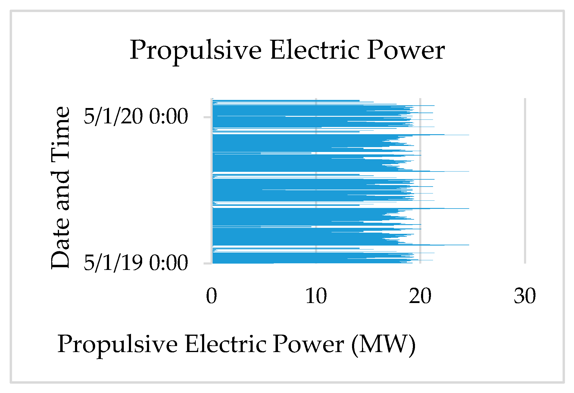
2.1. Ship, Route Description, and Energy Estimation
2.2. Diesel Generator
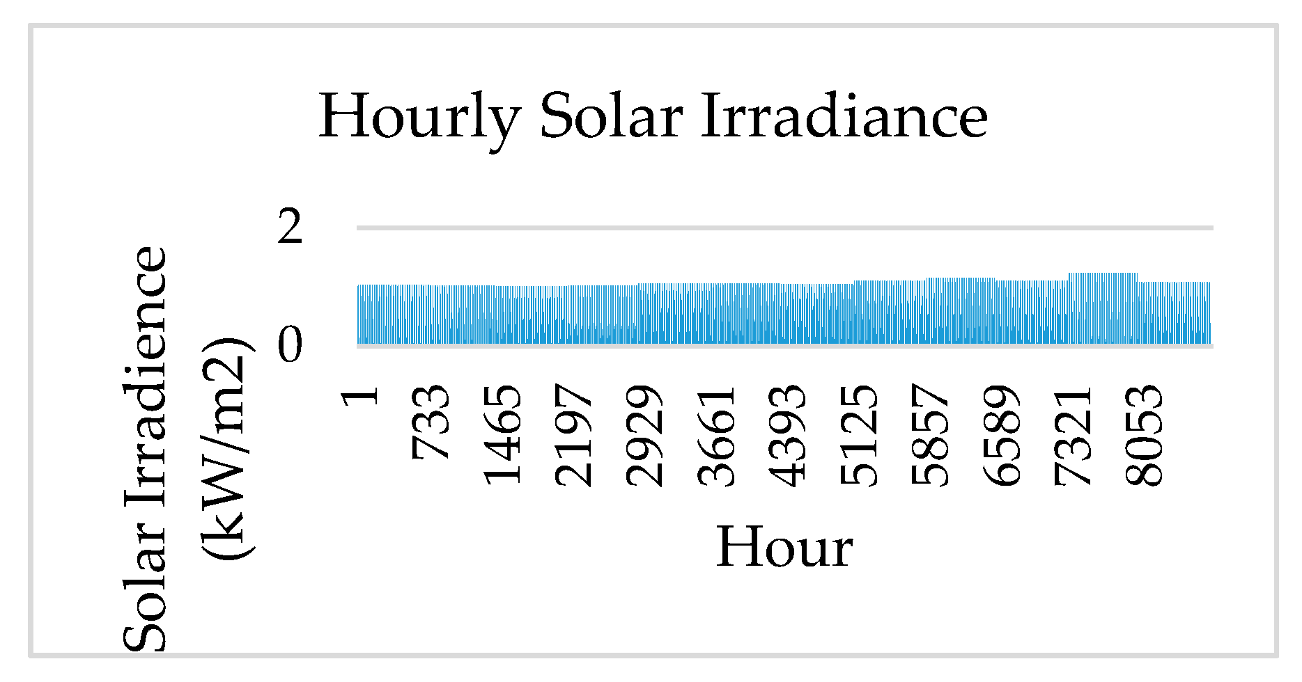
2.3. Solar Energy
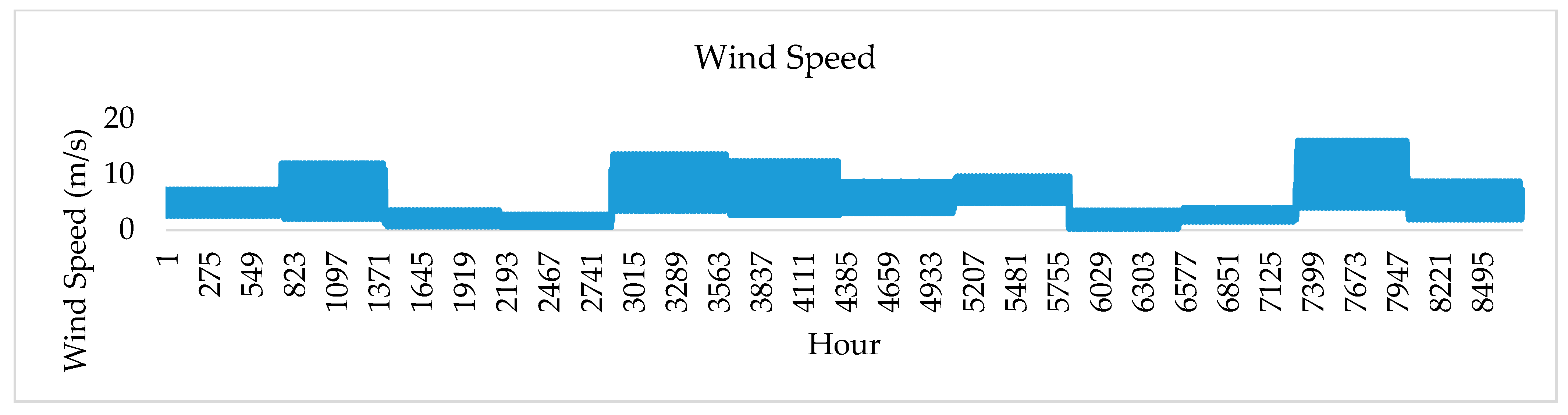
2.4. Wind Power
2.5. vSMR/MR
2.6. Electrochemical Energy Storage
3. Key Performance Indicators
3.1. Net Present Cost (NPC)/Net Present Value (NPV)
3.2. Levelized Cost of Energy (LCOE)
3.3. Generation Reliability Factor (GRF)
3.4. Loss of Power Supply Probability (LPSP)
3.5. CO2 Gas Emissions
3.6. Power to Weight Ratio (PWR)
4. Problem Formation
4.1. Objective Function
4.2. Constraints
4.3. Decision Variables
4.4. Implementation of Optimization Algorithm: Differential Evolution
| Step 1: | Read the following input data of the proposed energy systems:
|
| Step 2: | Initialize the parameters of DE and required system components:
|
| Step 3: | Generate the initial solutions randomly within the boundary of the decision variables. The number of the randomly generated solution is equal to the population size. These solutions are called target solutions. |
| Step 4: | Generate the donor solutions by mutating the target solutions. |
| Step 5: | Generate the trail solutions by recombing the donor the solutions (crossover). |
| Step 6: | Bound the trial solutions within the boundary of the decision variables. |
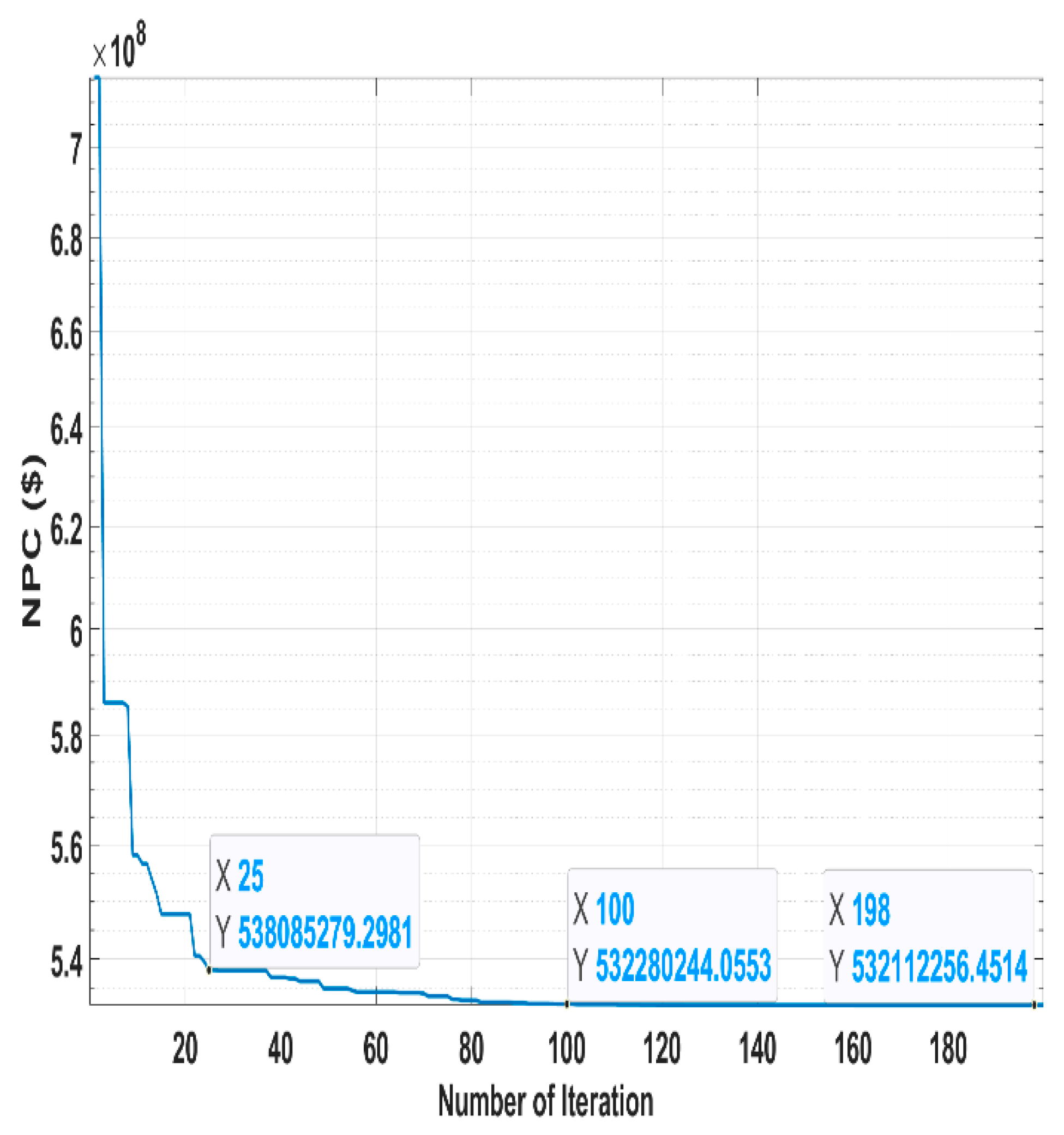
| Step 7: | Evaluate the objective function for the target solutions and trial solutions. The solution that gives the lower value (minimization problem) of the objective function is selected as the target solution for the next iteration. Store the best cost value (lowest value) in every iteration. |
| Step 8: | When the number of iteration reaches the maximum limit of the iteration, then stop. Otherwise, continue from Step 3 to Step 7. After completing all the iteration, the best objective function value is obtained, and the associated solution is the global optimal solution. |
4.5. Adaptive Differential Evolution
4.6. Implementation of Optimization Algorithm: Particle Swarm Optimization (PSO)
| Step 1: | Read the following input data of the proposed energy systems:
|
| Step 2: | Initialize the parameters of DE and required system components:
|
| Step 3: | Generate the initial solutions randomly within the boundary of the decision variables. |
| Step 4: | Use the individual particle position to determine the objective function value. |
| Step 5: | Update the best position of the individual particle by comparing it with all other populations. |
| Step 6: | Compare the personal best with the global best and update the global best with the individual particle’s personal best that has the minimum value of the objective function. |
| Step 7: | Update the velocity of the individual particle. |
| Step 8: | Update the position of the individual particle. |
| Step 9: | Repeat step 3 to step 8 till all particles are evaluated in each iteration. Store the best cost value. |
| Step 10: | Stop the simulation if it reaches the maximum number of iterations. |
5. Results
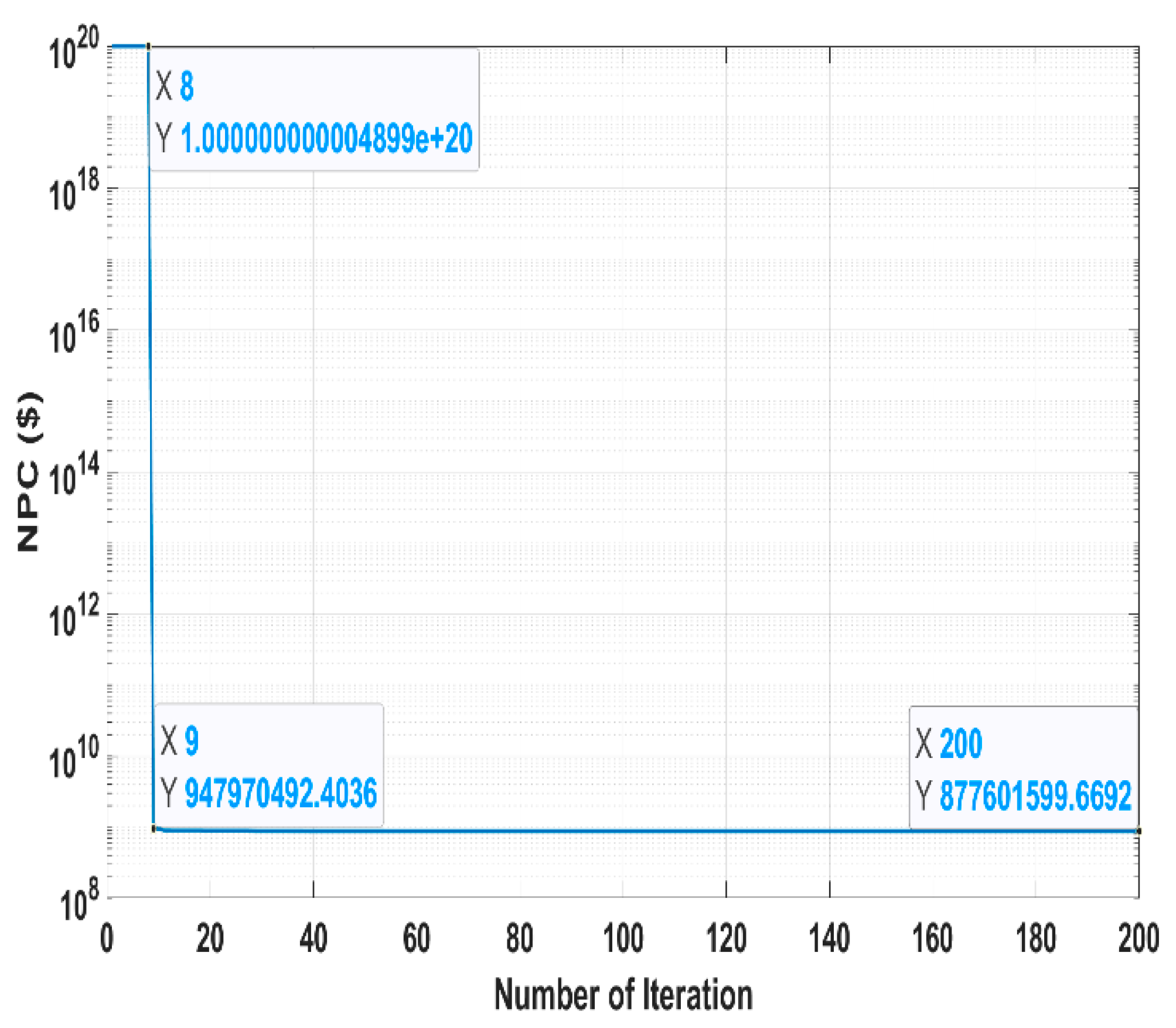
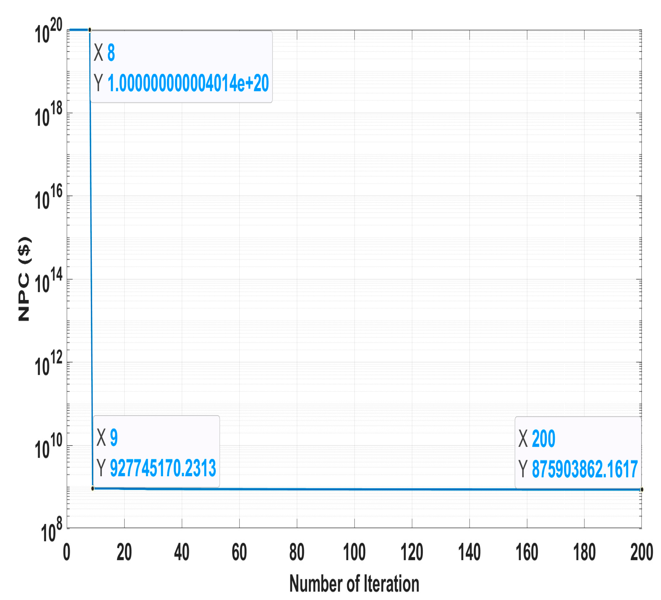
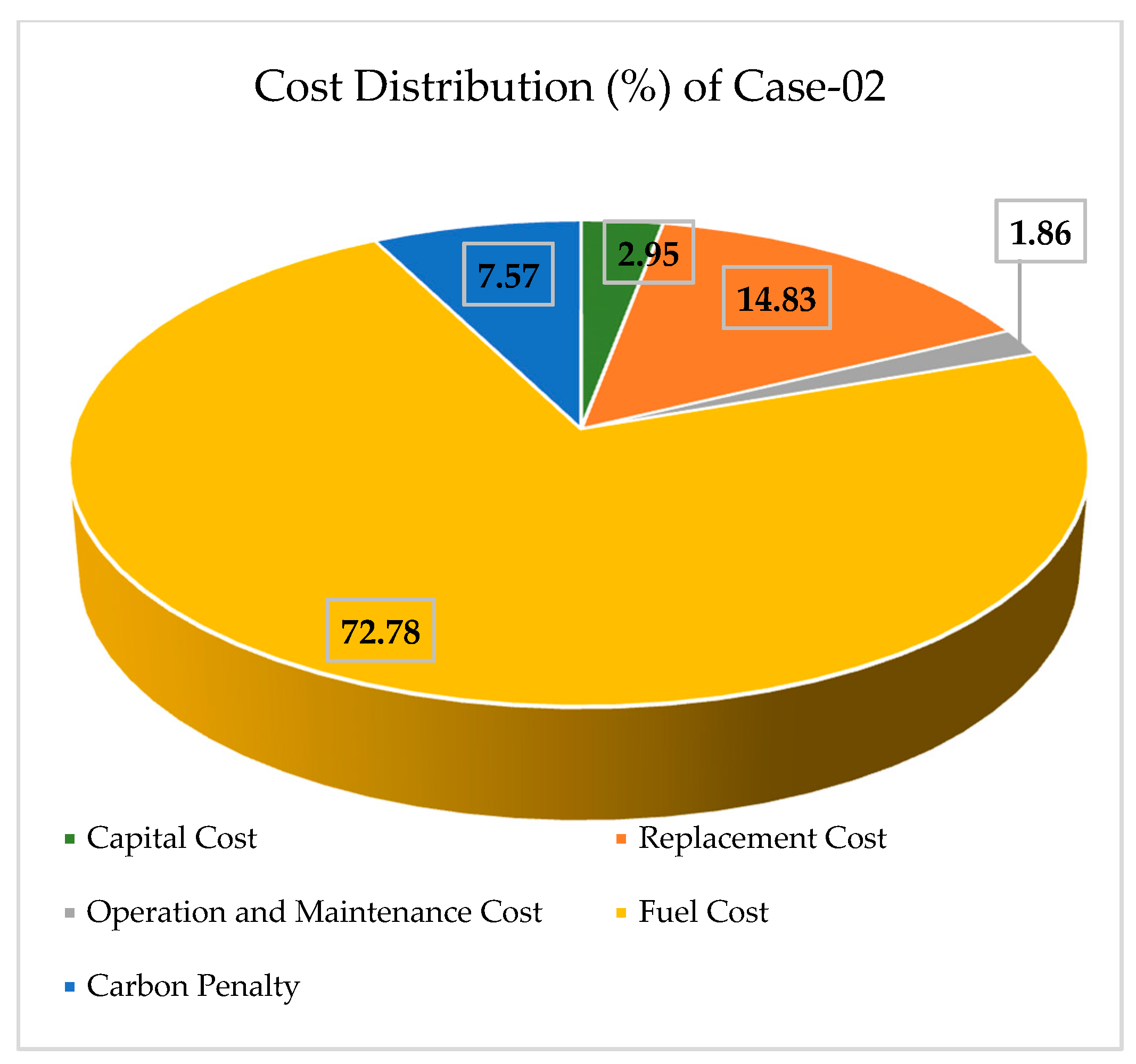
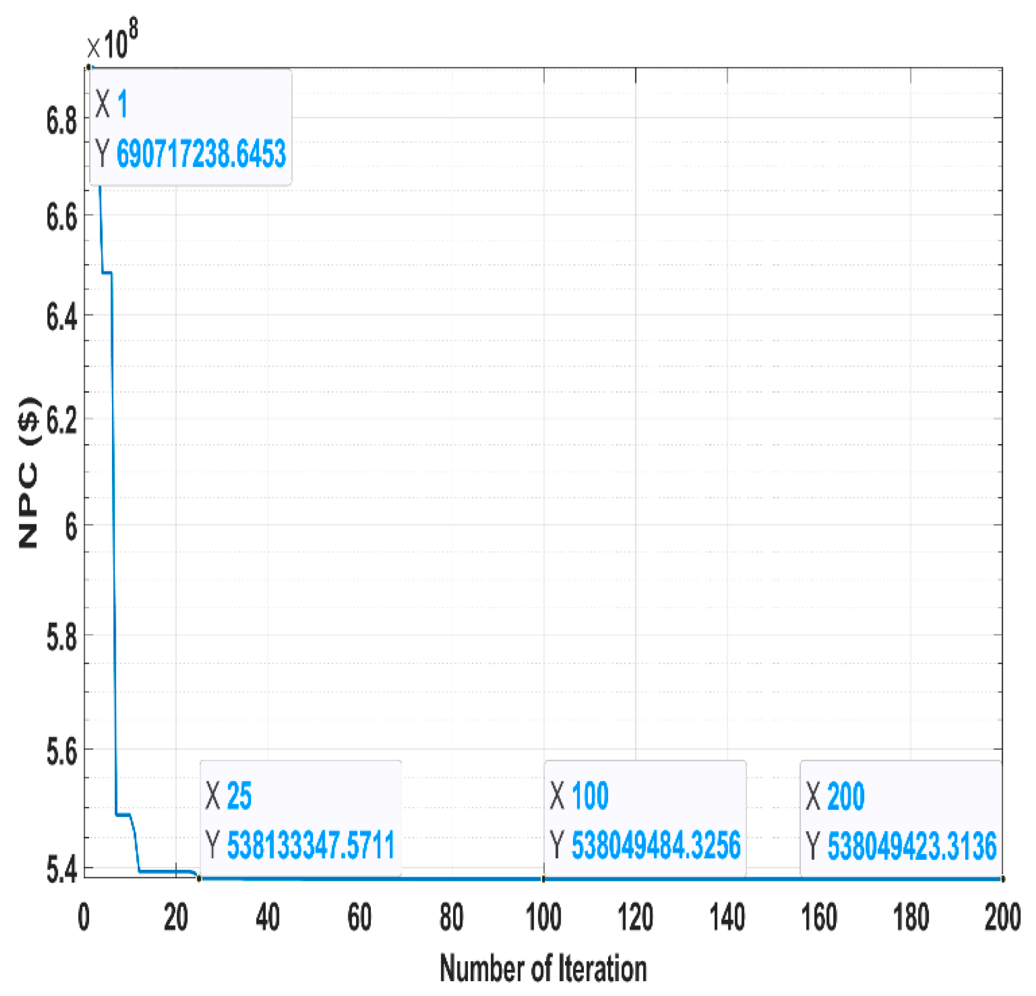
5.1. Comparison among the Proposed Hybrid Energy Systems
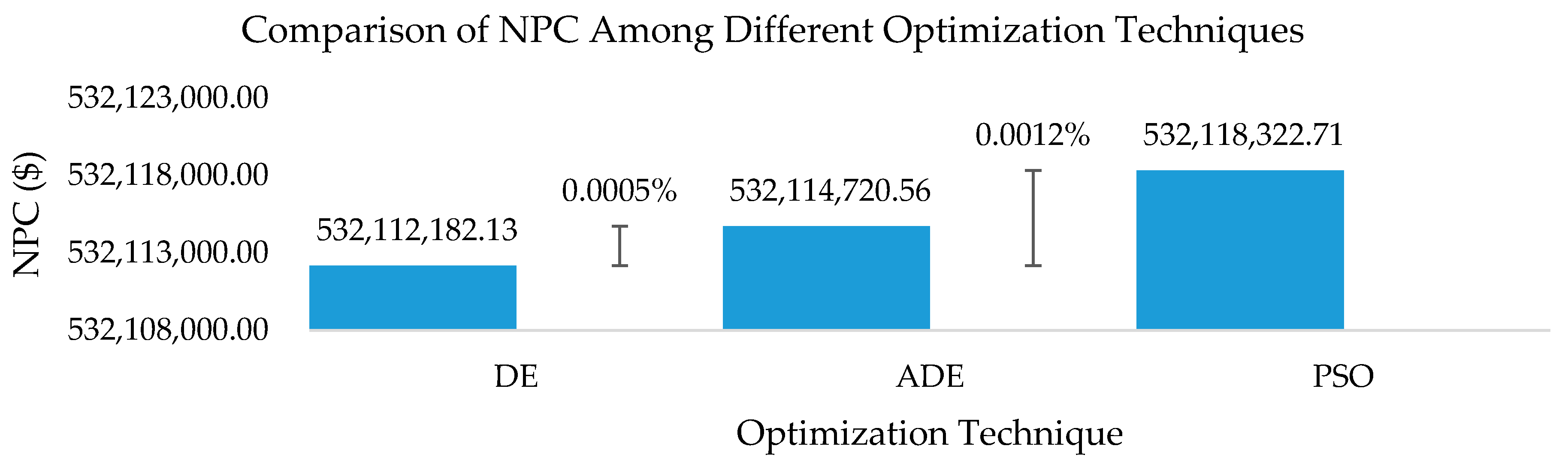
5.2. Comparison and Validation of Optimization Techniques
6. Sensitivity Analysis
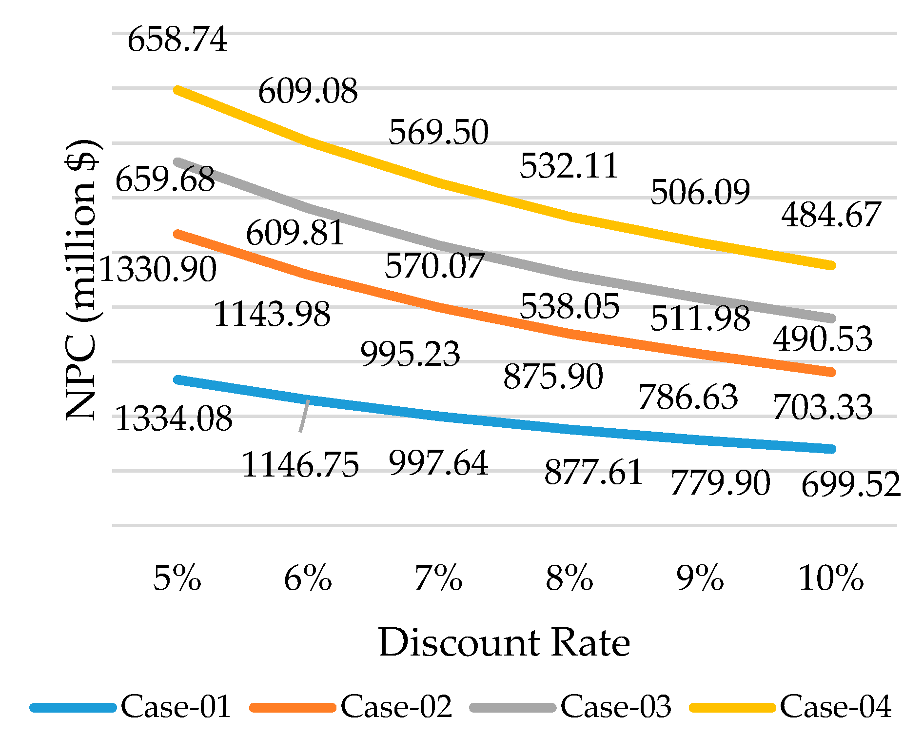
6.1. Sensitivity Assessment of Discount Rate on NPC
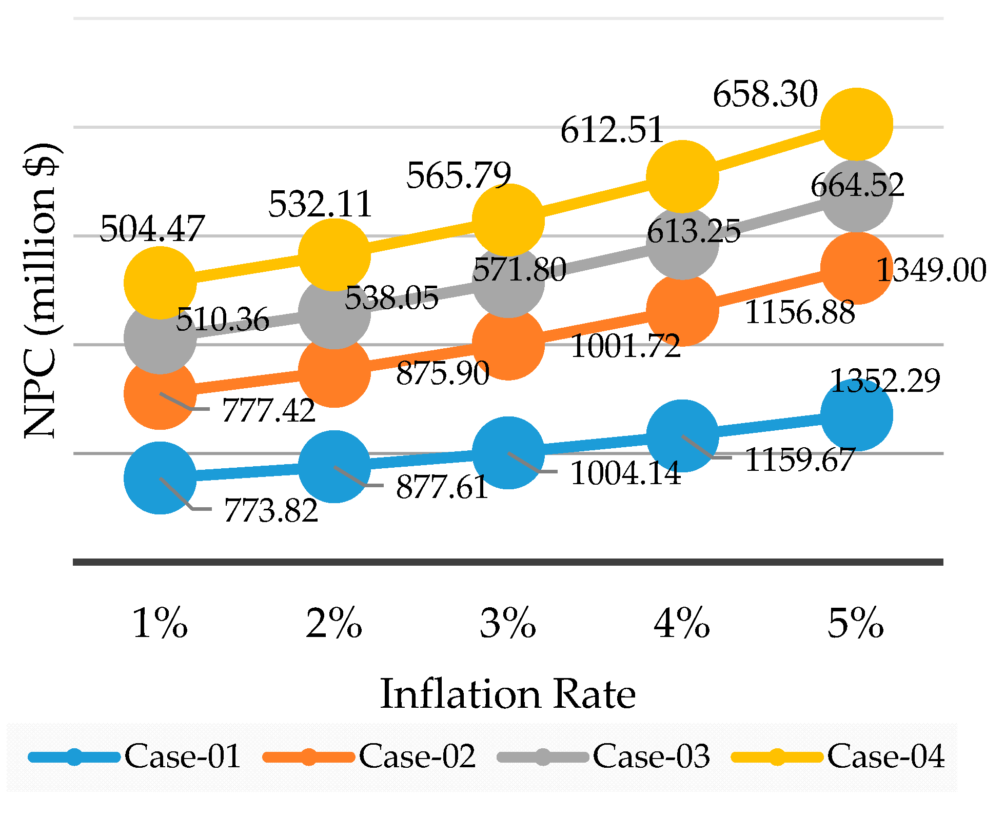
6.2. Sensitivity Assessment of Inflation Rate on NPC
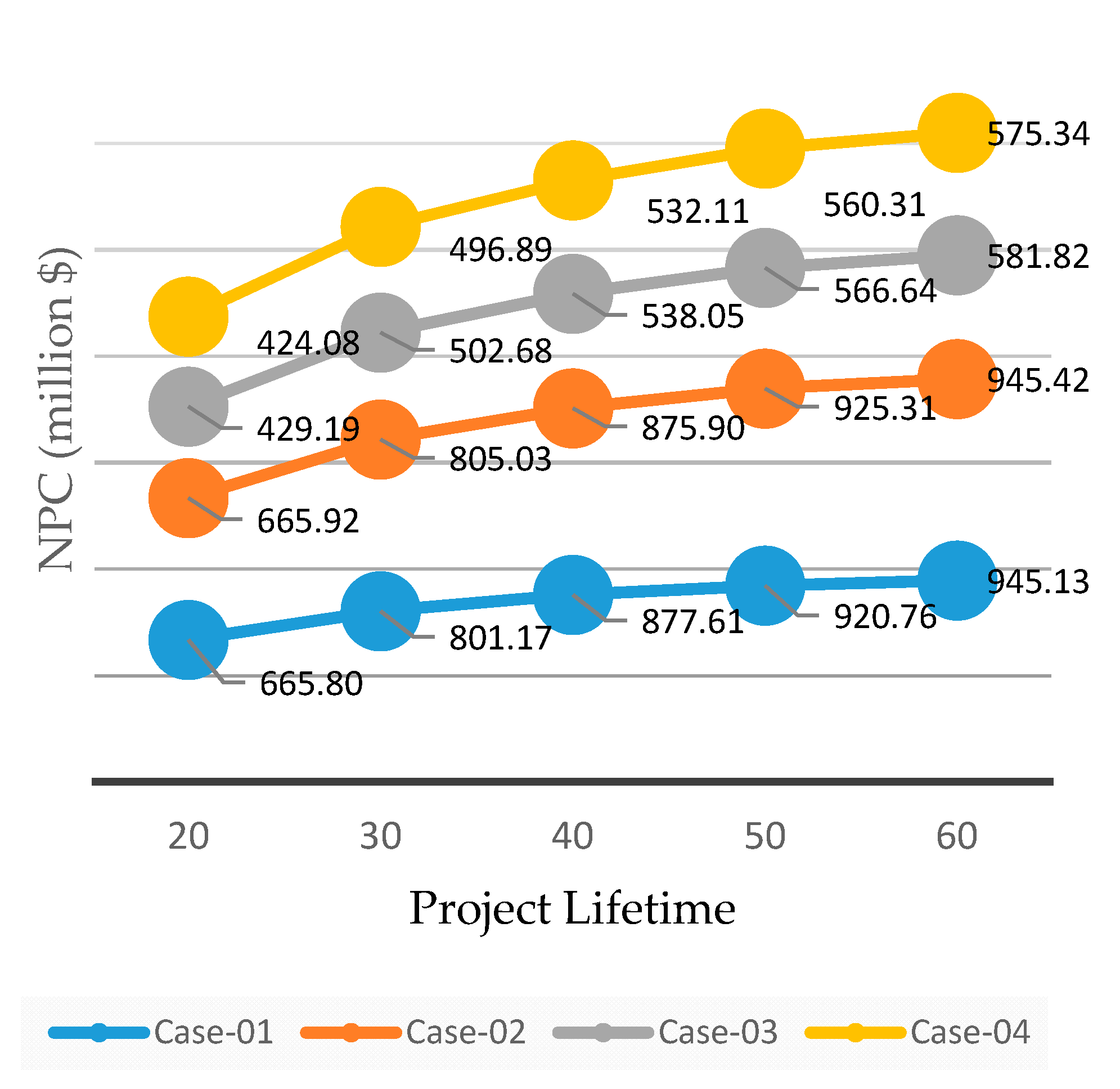
6.3. Sensitivity Assessment of Project Lifetime on NPC
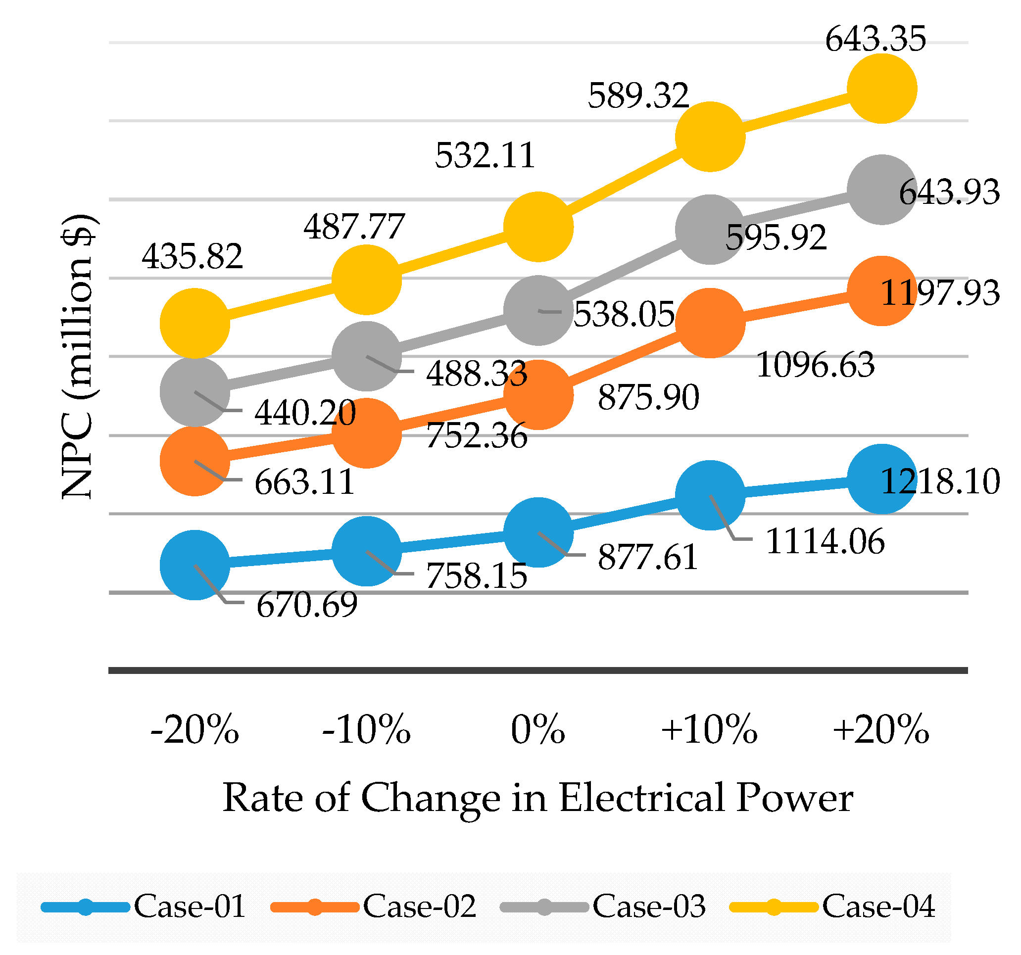
6.4. Sensitivity Assessment of Electrical Power Requirement on NPC
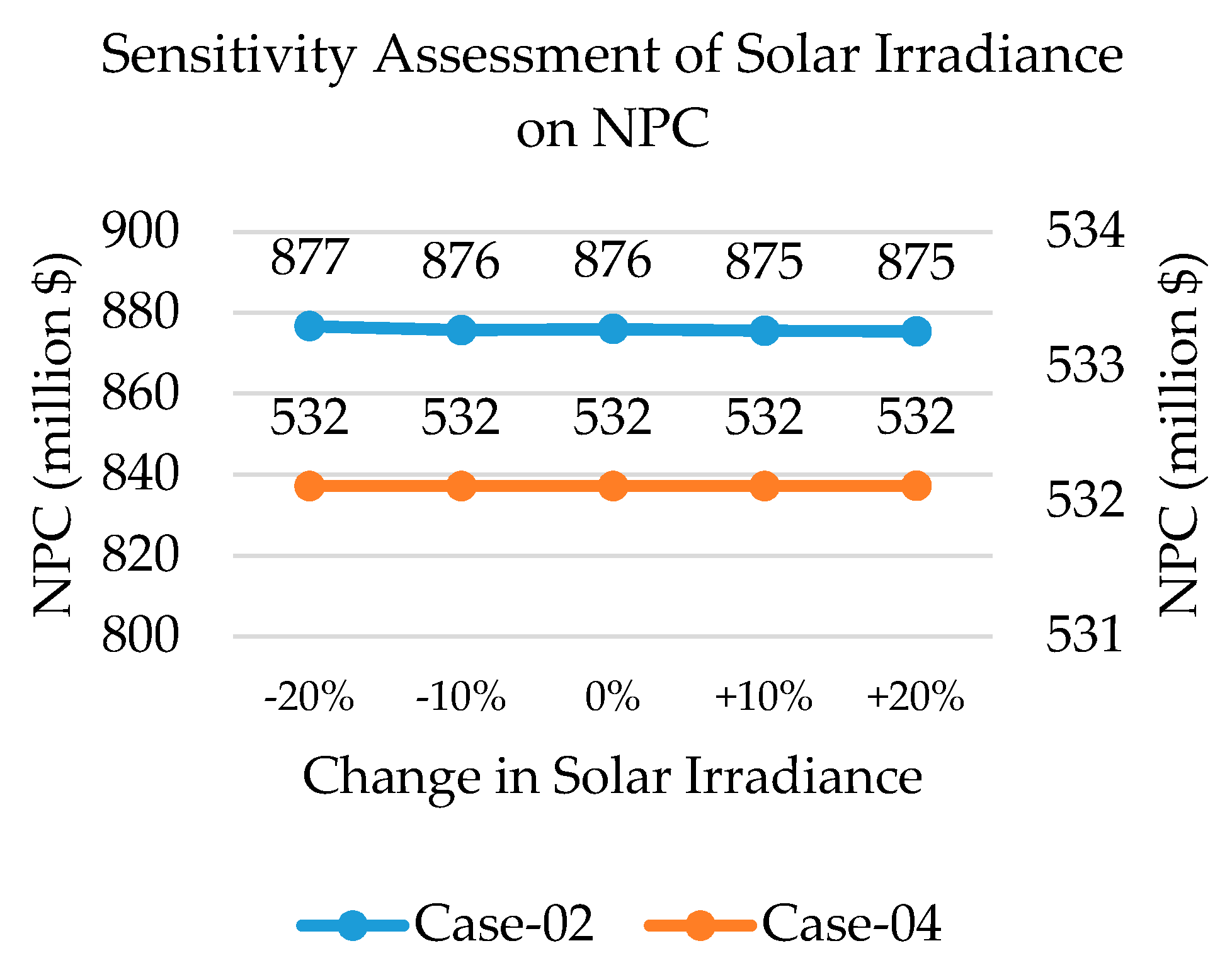
6.5. Sensitivity Assessment of Solar Irradiance on NPC
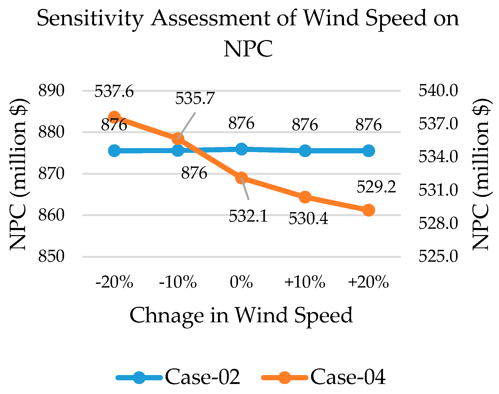
6.6. Sensitivity Assessment of Wind Speed on NPC
7. Conclusions, Contribution and Future Scope of Work
- ➢
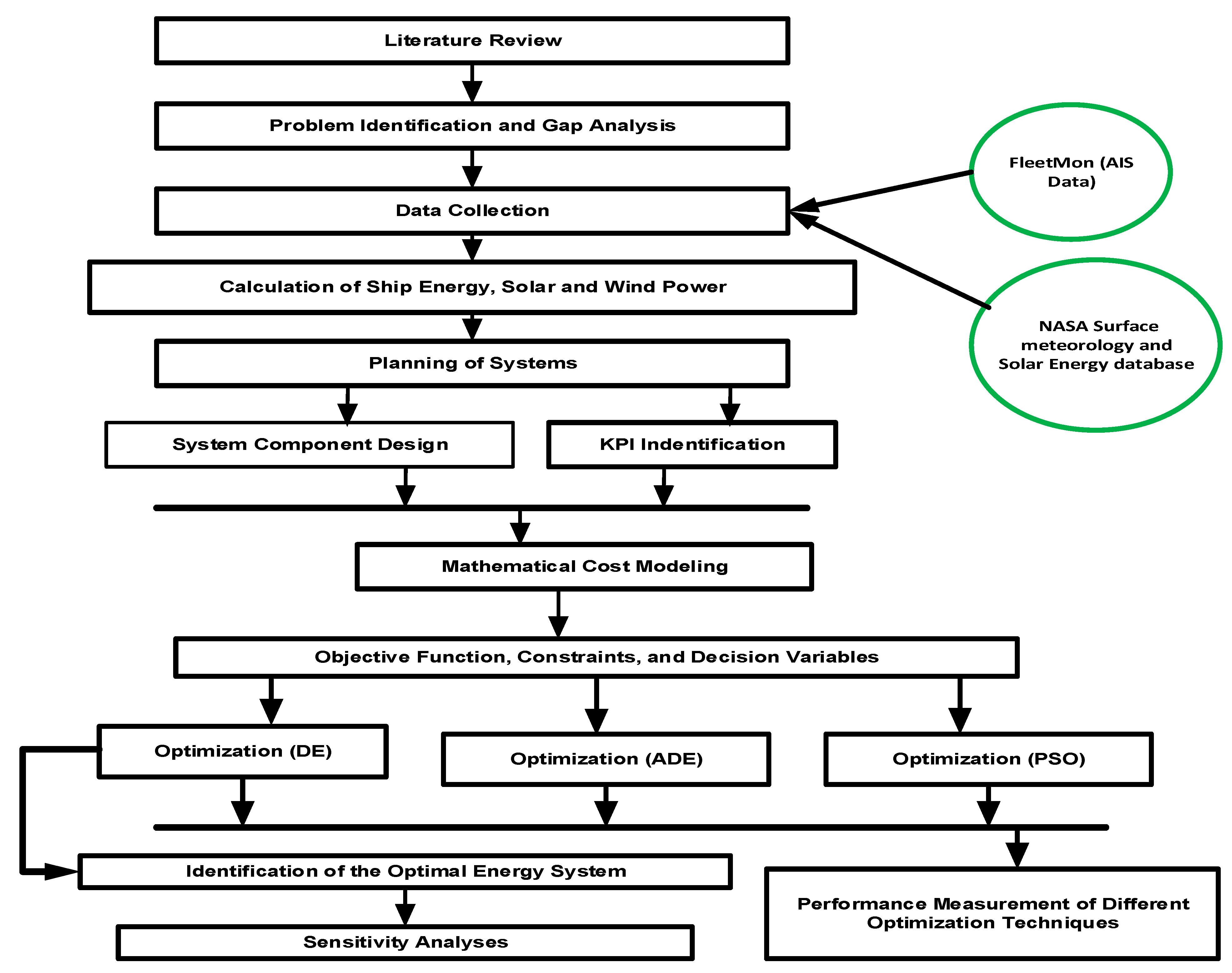
- A comprehensive literature review on the impact of maritime transportation on the environment, renewable and fossil fuel-based hybrid energy systems, nuclear propulsion, development of N-R HES in land-based applications to identify the problem and gaps.
- ➢
- Estimate the energy requirement of an oil tanker with the collaboration of industry (FleetMon) to address a real-world problem in this study.
- ➢
- Four energy systems are introduced to determine the most feasible energy system for maritime transportations. The feasibility is assessed based on technical, economical, and environmental KPIs. To ensure the reliability of the energy system, certain constraints are added.
- ➢
- The economical model of all the system components is developed mathematically. This mathematical model is then optimized in the popular and versatile simulator MATLAB. The Differential Evolution (DE) algorithm is used to optimize the energy systems.
- ➢
- The performance of the DE algorithm is compared to another optimization technique, PSO. Also, the impact of the control parameters of the DE algorithm is measured by the Adaptive Differential Algorithm (ADE).
- ➢
- To address the variability of the parameters like discount rate, inflation rate, project lifetime, electrical power requirements, solar irradiance, and wind speed, a sensitivity analysis is conducted to reinforce the findings.
- ➢
- In this study, average solar irradiance, temperature, and wind speed are used while optimizing the systems. In the future, the actual solar irradiance, temperature, and wind speed can be used to make the study more realistic.
- ➢
- In this study, a specific ship route is considered. However, analysis can be extended to different major international shipping routes to assess the most feasible route for N-R HES.
- ➢
- The safety of the N-R HES can be assessed in the future to check the feasibility in maritime transportation.
- ➢
- The licensing procedure and port approval of nuclear-powered merchant ships need to be addressed.
- ➢
- In this study, no secondary commodities are considered to utilize the excess heat of the nuclear reactor. In the future, the excess energy can be utilized to produce secondary commodities like seawater desalination or utilize it by using in heating and cooling system.
Author Contributions
Funding
Institutional Review Board Statement
Informed Consent Statement
Data Availability Statement
Conflicts of Interest
Nomenclature
| AIS | Automatic Identification System |
| FFG | Fossil Fuel-based Generator |
| GHG | Greenhouse Gas |
| GRF | Generation Reliability Factor |
| HES | Hybrid Energy System |
| IAEA | International Atomic Energy Agency |
| KPI | Key Performance Indicator |
| LBP | Length Between Perpendiculars |
| MR | Microreactor |
| MT | Metric Ton |
| NASA | National Aeronautics and Space Administration |
| NPC | Net Present Cost |
| NPP | Nuclear Power Plant |
| NPV | Net Present Value |
| N-R HES | Nuclear-Renewable Hybrid Energy System |
| N-R HES | Nuclear-Renewable Hybrid Energy System |
| RES | Renewable Energy Source |
| RINA | Royal Institution of Naval Architects |
| SMR | Small Modular Reactor |
Appendix A

| SL. No | Parameter/Assumption | Category | Notation | Value | Reference |
|---|---|---|---|---|---|
| 1 | Ship beam | Parameter | B | 60 m | [72] |
| 2 | Volume displacement | Parameter | v | 344,649.08 m3 | [72] |
| 3 | Draught | Parameter | D | 21.6 m | [15] |
| 4 | Extreme breadth (Beam) | Parameter | Bex | 60.04 m | [72] |
| 5 | Average draught | Parameter | D_avg | 16.15 m | [15] |
| 6 | Length between perpendiculars | Parameter | LBP | 324 m | [72] |
| 7 | Gravitational acceleration | Parameter | g | 9.81 m/s2 | |
| 8 | Seawater density at 30 °C temperature | Parameter | ρw | 1021.7 kg/m3 | [17] |
| 9 | Seawater viscosity at 30 °C temperature | Parameter | γw | 0.84931 × 10⁻⁶ m3s−1 | [17] |
| 10 | Average speed | Parameter | Vs_avg | 11.94 kn or 6.1424 ms−1 | [15] |
| 11 | Incremental resistance coefficient due to surface roughness of ship | Assumption | CA | 0.0004 | [17] |
| 12 | Maximum speed | Parameter | Vs_max | 17.9 kn or 9.2185 ms−1 | [15] |
Appendix B


Appendix C


Appendix D
References
- Shipping Pollution. OCEANA Protecting the World’s Ocean. Available online: https://europe.oceana.org/en/shipping-pollution-1 (accessed on 17 October 2020).
- Yuan, J.; Ng, S.H.; Sou, W.S. Uncertainty quantification of CO2 emission reduction for maritime shipping. Energy Policy 2016, 88, 113–130. [Google Scholar] [CrossRef]
- Koumentakos, A.G. Developments in Electric and Green Marine Ships. Appl. Syst. Innov. 2019, 2, 34. [Google Scholar] [CrossRef]
- FUTURE SHIP POWERING OPTIONS Exploring Alternative Methods of Ship Propulsion. July 2013. Available online: https://www.raeng.org.uk/publications/reports/future-ship-powering-options (accessed on 12 April 2021).
- Batteries on Board Ocean-Going Vessels. Available online: https://www.man-es.com/docs/default-source/marine/tools/batteries-on-board-ocean-going-vessels.pdf?sfvrsn=deaa76b8_12 (accessed on 4 March 2021).
- Borowski, P.F. Zonal and Nodal Models of Energy Market in European Union. Energies 2020, 13, 4182. [Google Scholar] [CrossRef]
- Gravina, J.; Blake, J.I.R.; Shenoi, A.; Turnock, S.R.; Hirdaris, S.E. Concepts for a modular nuclear powered containership. In Proceedings of the 17th International Conference on Ships and Shipping Research (NAV 2012), Napoli, Italy, 17–19 October 2012. [Google Scholar]
- Luciano Ondir Freire and Delvonei Alves de Andrade. Historic survey on nuclear merchant ships. Nucl. Eng. Des. 2015, 293, 176–186. [Google Scholar] [CrossRef]
- Hirdaris, S.E.; Cheng, Y.F.; Shallcross, P.; Bonafoux, J.; Carlson, D.; Prince, B.; Sarris, G.A. Considerations on the potential use of Nuclear Small Modular Reactor (SMR) technology for merchant marine propulsion. Ocean Eng. 2014, 79, 101–130. [Google Scholar] [CrossRef]
- Chaouki, G.; Maamar, B.; Boris, B.; Abdul, K.H. Hybrid solar PV/PEM fuel Cell/Diesel Generator power system for cruise ship: A case study in Stockholm, Sweden. Case Stud. Therm. Eng. 2019, 14, 100497. [Google Scholar] [CrossRef]
- Diab, F.; Lan, H.; Ali, S. Novel comparison study between the hybrid renewable energy systems on land and on ship. Renew. Sustain. Energy Rev. 2016, 63, 452–463. [Google Scholar] [CrossRef]
- Boldon, L.; Sabharwall, P.; Bragg-Sitton, S.; Abreu, N.; Liu, L. Nuclear Renewable Energy Integration: An Economic Case Study. Int. J. Energy Environ. Econ. 2015, 28, 85–95. [Google Scholar]
- Gabbar, H.A.; Abdussami, M.R.; Adham, M.I. Micro Nuclear Reactors: Potential Replacements for Diesel Gensets within Micro Energy Grids. Energies 2020, 13, 5172. [Google Scholar] [CrossRef]
- Gabbar, H.A.; Abdussami, M.R.; Adham, M.I. Optimal Planning of Nuclear-Renewable Micro-Hybrid Energy System by Particle Swarm Optimization. IEEE Access 2020, 8, 181049–181073. [Google Scholar] [CrossRef]
- Voyage Analyser DEMO. Available online: https://voyage.vesselfinder.com/3a9abdd131b21a2a4f7d6acf52f0d2d2 (accessed on 17 October 2020).
- Gabbar, H.A.; Adham, M.I.; Abdussami, M.R. Analysis of nuclear-renewable hybrid energy system for marine ships. Energy Rep. 2021, 7, 2398–2417. [Google Scholar] [CrossRef]
- Chuku, A.J.; Ukeh, M.E.; Mkpa, A. Estimation of bare hull resistance of a ropax vessel using the ittc-57 method and gertler series data chart. Energy Rep. 2017, 3, 406–422. [Google Scholar]
- Molland, A.F.; Turnock, S.R.; Hudson, D.A. Ship Resistance and Propulsion, Practical Estimation of Ship Propulsive Power; Cambridge University Press: Cambridge, UK, 2014; Chapter 10; p. 207. [Google Scholar]
- Nicewicz, G.; Tarnapowicz, D. Assessment of Marine Auxiliary Engines Load Factor in Ports. Available online: https://www.researchgate.net/publication/298026922_Assessment_of_marine_auxiliary_engines_load_factor_in_ports (accessed on 22 December 2020).
- Moore, M. The Economics of Very Small Modular Reactors In The North. Canadian Nuclear Laboratories, Delta Ottawa City Centre Hotel CW-120200-CONF-012 Ottawa, Ontario, Canada, November 2016. Available online: https://inis.iaea.org/search/search.aspx?orig_q=RN:49103606 (accessed on 25 December 2020).
- Heydari, A.; Askarzadeh, A. Optimization of a biomass-based photovoltaic power plant for an off-grid application subject to loss of power supply probability concept. Appl. Energy 2016, 165, 601–611. [Google Scholar] [CrossRef]
- Lan, H.; Wen, S.; Hong, Y.; Yu, D.C.; Zhang, L. Optimal sizing of hybrid PV/diesel/battery in ship power system. Appl. Energy 2015, 158, 26–34. [Google Scholar] [CrossRef]
- Markvart, T. Solar Electricity; John Wiley & Sons: Hoboken, NJ, USA, 2000. [Google Scholar]
- Gabbar, H.A.; Abdussami, M.R.; Adham, M.I. Techno-Economic Evaluation of Interconnected Nuclear-Renewable Micro Hybrid Energy Systems with Combined Heat and Power. Energies 2020, 13, 1642. [Google Scholar] [CrossRef]
- Solar Panel Maintenance Costs | Solar Power Maintenance Estimates. Fixr.com. Available online: https://www.fixr.com/costs/solar-panel-maintenance (accessed on 16 April 2020).
- What Is the Lifespan of a Solar Panel? Available online: https://www.engineering.com/DesignerEdge/DesignerEdgeArticles/ArticleID/7475/What-Is-the-Lifespan-of-a-Solar-Panel.aspx (accessed on 16 April 2020).
- SUN2000-(25KTL, 30KTL)-US, User Manual. HUAWEI TECHNOLOGIES CO., LTD. 1 April 2017. Available online: https://www.huawei.com/minisite/solar/en-na/service/SUN2000-25KTL-30KTL-US/User_Manual.pdf (accessed on 29 May 2021).
- Kobougias, I.; Tatakis, E.; Prousalidis, J. PV Systems Installed in Marine Vessels: Technologies and Specifications. Adv. Power Electron. 2013, 2013, 831560. [Google Scholar] [CrossRef]
- Lu, L.; Yang, H.; Burnett, J. Investigation on wind power potential on Hong Kong islands—An analysis of wind power and wind turbine characteristics. Renew. Energy 2002, 27, 1–12. [Google Scholar] [CrossRef]
- Borowy, B.S.; Salameh, Z.M. Methodology for optimally sizing the combination of a battery bank and PV array in a Wind/PV hybrid system. IEEE Trans. Energy Convers. 1996, 11. [Google Scholar] [CrossRef]
- Yang, H.; Lu, L.; Zhou, W. A novel optimization sizing model for hybrid solar-wind power generation system. Sol. Energy 2007, 81, 76–84. [Google Scholar] [CrossRef]
- Yang, H.X.; Lu, L.; Burnett, J. Weather data and probability analysis of hybrid photovoltaic–wind power generation systems in Hong Kong. Renew. Energy 2003, 28, 1813–1824. [Google Scholar] [CrossRef]
- Mukhtaruddin, R.N.S.R.; Rahman, H.A.; Hassan, M.Y.; Jamian, J.J. Optimal hybrid renewable energy design in autonomous system using Iterative-Pareto-Fuzzy technique. Int. J. Electr. Power Energy Syst. 2015, 64, 242–249. [Google Scholar] [CrossRef]
- Bauer, L. Endurance E-3120—50.00 kW—Wind Turbine. Available online: https://en.wind-turbine-models.com/turbines/372-endurance-e-3120 (accessed on 6 March 2021).
- N. E. B. Government of Canada. NEB—Market Snapshot: The Cost to Install Wind and Solar Power in Canada is Projected to Significantly Fall Over the Long Term. 13 February 2020. Available online: https://www.cer-rec.gc.ca/nrg/ntgrtd/mrkt/snpsht/2018/11-03cstnstllwnd-eng.html (accessed on 24 July 2020).
- US Wind O&M Costs Estimated at $48,000/MW; Falling Costs Create New Industrial Uses: IEA | New Energy Update. Available online: https://analysis.newenergyupdate.com/wind-energy-update/us-wind-om-costs-estimated-48000mw-falling-costs-create-new-industrial-uses-iea (accessed on 17 April 2020).
- Stehly, T.; Beiter, P.; Heimiller, D.; Scott, G. 2017 Cost of Wind Energy Review. Renew. Energy 2018. [Google Scholar] [CrossRef]
- Stackhouse, P.W. Surface Meteorology and Solar Energy (SSE) Data Release 5.1. Available online: https://ntrs.nasa.gov/search.jsp?R=20080012141 (accessed on 24 July 2020).
- Aeolos Wind Turbine Company—50kw Wind Turbine—Wind Power Generation—Aeolos 50 kw Turbine Wind Energy. Available online: https://www.windturbinestar.com/50kwh-aeolos-wind-turbine.html (accessed on 6 March 2021).
- Diaf, S.; Notton, G.; Belhamel, M.; Haddadi, M.; Louche, A. Design and techno-economical optimization for hybrid PV/wind system under various meteorological conditions. Appl. Energy 2008, 85, 968–987. [Google Scholar] [CrossRef]
- World Nuclear Association. Small Nuclear Power Reactors. Available online: https://www.world-nuclear.org/information-library/nuclear-fuel-cycle/nuclear-power-reactors/small-nuclear-power-reactors.aspx (accessed on 25 December 2020).
- Microreactors Frequently Asked Questions | Microreactors. Available online: https://inl.gov/trending-topic/microreactors/frequently-asked-questions-microreactors/ (accessed on 25 December 2020).
- Cost Competitiveness of Micro-Reactors for Remote Markets. Available online: https://www.nei.org/resources/reports-briefs/cost-competitiveness-micro-reactors-remote-markets (accessed on 6 March 2021).
- Borhanazad, H.; Mekhilef, S.; Ganapathy, V.G.; Modiri-Delshad, M.; Mirtaheri, A. Optimization of micro-grid system using MOPSO. Renew. Energy 2014, 71, 295–306. [Google Scholar] [CrossRef]
- Marine Electrical Technology. Available online: https://www.goodreads.com/work/best_book/10132141-marine-electrical-technology (accessed on 6 March 2021).
- Ship’s Emergency Power. DieselShipDieselShip, Connecting Mariners Worldwide. Available online: https://dieselship.com/marine-technical-articles/marine-electro-technology/ships-emergency-power/ (accessed on 1 January 2021).
- PV. Performance Modeling Collaborative. CEC Inverter Test Protocol. Available online: https://pvpmc.sandia.gov/modeling-steps/dc-to-ac-conversion/cec-inverter-test-protocol/ (accessed on 1 January 2021).
- Luo, X.; Wang, J.; Dooner, M.; Clarke, J. Overview of current development in electrical energy storage technologies and the application potential in power system operation. Appl. Energy 2015, 511–536. [Google Scholar] [CrossRef]
- Net Present Value (NPV). What is Net Present Value (NPV)? Available online: https://corporatefinanceinstitute.com/resources/knowledge/valuation/net-present-value-npv/ (accessed on 3 January 2021).
- Converting Nominal Interest Rates to Real Interest Rates | TVMCalcs.com. Available online: http://www.tvmcalcs.com/index.php/calculators/apps/converting_nominal_interest_rates_to_real_interest_rates (accessed on 11 May 2021).
- Luna-Rubio, R.; Trejo-Perea, M.; Vargas-Vázquez, D.; Ríos-Moreno, G.J. Optimal sizing of renewable hybrids energy systems: A review of methodologies. Sol. Energy 2012, 86, 1077–1088. [Google Scholar] [CrossRef]
- Oria, J.; Madariaga, E.; Ortega, A.; Díaz, E.; Mateo, M. Influence of characteristics of marine auxiliary power system in the energy efficiency design index. J. Marit. Transp. Eng. 2015, 4, 67. [Google Scholar]
- Godsey, K.M. Life Cycle Assessment of Small Modular Reactors Using U.S. Nuclear Fuel Cycle. Clemson University. Available online: https://core.ac.uk/download/pdf/287319878.pdf (accessed on 26 December 2020).
- Parry, I. Countries Are Signing Up for Sizeable Carbon Prices. Available online: https://blogs.imf.org/2016/04/21/countries-are-signing-up-for-sizeable-carbon-prices/#more-12399 (accessed on 6 January 2021).
- IMF Calls for Carbon Tax on Ships and Planes. Available online: https://www.theguardian.com/environment/2016/jan/13/imf-calls-for-carbon-tax-on-ships-and-planes (accessed on 17 October 2020).
- Marine Insights. 14 Terminologies Used for Power of the Ship’s Marine Propulsion Engine. Available online: https://www.marineinsight.com/main-engine/12-terminologies-used-for-power-of-the-ships-marine-propulsion-engine/ (accessed on 7 January 2021).
- FANDOM. Power-to-Weight Ratio. Available online: https://automobile.fandom.com/wiki/Power-to-weight_ratio (accessed on 7 January 2021).
- Salvage Value. Available online: https://www.homerenergy.com/products/pro/docs/latest/salvage_value.html (accessed on 13 July 2020).
- Rubin, E.S.; Azevedo, I.M.L.; Jaramillo, P.; Yeh, S. A review of learning rates for electricity supply technologies. Energy Policy 2015, 86, 198–218. [Google Scholar] [CrossRef]
- Abdelshafy, A.M.; Hassan, H.; Mohamed, A.M.; El-Saady, G.; Ookawara, S. Optimal grid connected hybrid energy system for Egyptian residential area. In Proceedings of the 2017 International Conference on Sustainable Energy Engineering and Application (ICSEEA), Jakarta, Indonesia, 23–26 October 2017; pp. 52–60. [Google Scholar] [CrossRef]
- NEI. Land Needs for Wind, Solar Dwarf Nuclear Plant’s Footprint. Available online: https://www.nei.org/news/2015/land-needs-for-wind-solar-dwarf-nuclear-plants#:~:text=A%20nuclear%20energy%20facility%20has,1%2C000%20megawatts%20of%20installed%20capacity.&text=A%20solar%20PV%20facility%20must,45%20and%2075%20square%20miles (accessed on 13 January 2021).
- Solar Panel Size Guide: How Big Is a Solar Panel? Available online: https://www.wholesalesolar.com/blog/solar-panel-size-guide (accessed on 3 May 2021).
- Greco, R.; Vanzi, I. New few parameters differential evolution algorithm with application to structural identification. J. Traffic Transp. Eng. 2019, 6, 1–14. [Google Scholar] [CrossRef]
- Huang, Z.; Chen, Y. An Improved Differential Evolution Algorithm Based on Adaptive Parameter. J. Control Sci. Eng. 2013, 2013, 462706. Available online: https://www.hindawi.com/journals/jcse/2013/462706/ (accessed on 1 March 2021). [CrossRef]
- Deng, W.; Xu, J.; Gao, X.-Z.; Zhao, H. An Enhanced MSIQDE Algorithm With Novel Multiple Strategies for Global Optimization Problems. IEEE Trans. Syst. Man Cybern. Syst. 2020, 1–10. [Google Scholar] [CrossRef]
- Mansueto, P.; Schoen, F. Memetic differential evolution methods for clustering problems. Pattern Recognit. 2021, 114, 107849. [Google Scholar] [CrossRef]
- Shukla, S.; Pandit, M. Multi-objective fuzzy rank based scheduling of utility connected microgrid with high renewable energy using differential evolution with dynamic mutation. Int. Trans. Electr. Energy Syst. 2021, 31, e12787. [Google Scholar] [CrossRef]
- Wang, L.; Hu, H.; Liu, R.; Zhou, X. An improved differential harmony search algorithm for function optimization problems. Soft Comput. 2019, 23, 4827–4852. [Google Scholar] [CrossRef]
- Deng, W. Quantum differential evolution with cooperative coevolution framework and hybrid mutation strategy for large scale optimization. Knowl. Based Syst. 2021, 224, 107080. [Google Scholar] [CrossRef]
- Rini, D.P.; Shamsuddin, S.M. Particle Swarm Optimization: Technique, System and Challenges. IJAIS 2011, 1, 33–45. [Google Scholar] [CrossRef]
- Pranava, G.; Prasad, P.V. Constriction Coefficient Particle Swarm Optimization for Economic Load Dispatch with valve point loading effects. In Proceedings of the 2013 International Conference on Power, Energy and Control (ICPEC), Dindigul, India, 6–8 February 2013; pp. 350–354. [Google Scholar] [CrossRef]
- Auke Visser’s International Super Tankers. Available online: http://www.aukevisser.nl/supertankers/VLCC%20T-V/id1147.htm (accessed on 17 October 2020).
- Maisler, J. Small Modular Reactors. Available online: http://hpschapters.org/florida/6spring.pdf (accessed on 7 January 2021).
- RTA84T. Available online: https://pdf.nauticexpo.com/pdf/waertsilae-corporation/rta84t/24872-12529.html#https://img.nauticexpo.com/pdf/repository_ne/24872/rta84t-12529_1b.jpg (accessed on 16 October 2020).
- Canadian Solar CS6U-335P Silver Poly Solar Panel. Available online: https://www.wholesalesolar.com/1930010/canadian-solar/solar-panels/canadian-solar-cs6u-335p-silver-poly-solar-panel (accessed on 16 October 2020).
- National Wind Watch. Available online: https://www.wind-watch.org/faq-size.php (accessed on 16 October 2020).


| Parameter | Case-01 | Case-02 | Case-03 | Case-04 |
|---|---|---|---|---|
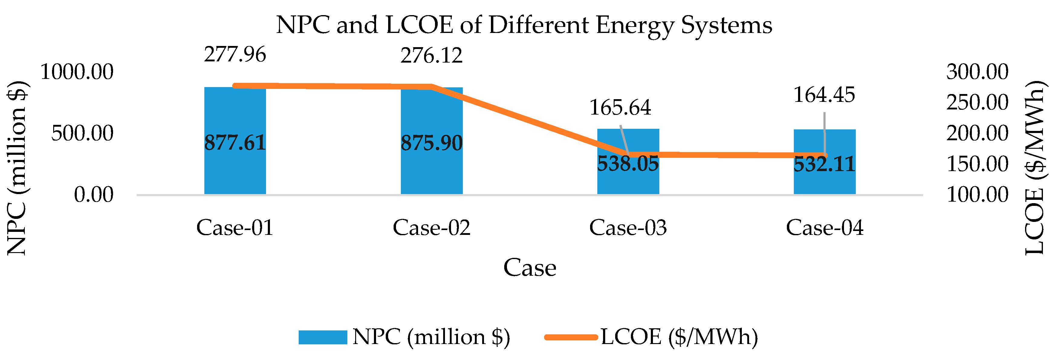
| NPC ($) | 877,605,291.05 | 875,903,862.16 | 538,049,423.31 | 532,112,182.13 |
| LCOE ($/MWh) | 277.96 | 276.12 | 165.64 | 164.45 |
| Generator/MMR (MW) | 28.15 | 28.14 | 28.96 | 28.00 |
| Solar PV (kW) | 0.00 | 396.79 | 0.00 | 0.0885334416 |
| Wind (kW) | 0.00 | 0.00 | 0.00 | 3050.30 |
| Battery (kWh) | 2341.38 | 3907.92 | 637.17 | 1351.92 |
| Solar ratio | N/A | 0.10 | N/A | 0.000022 |
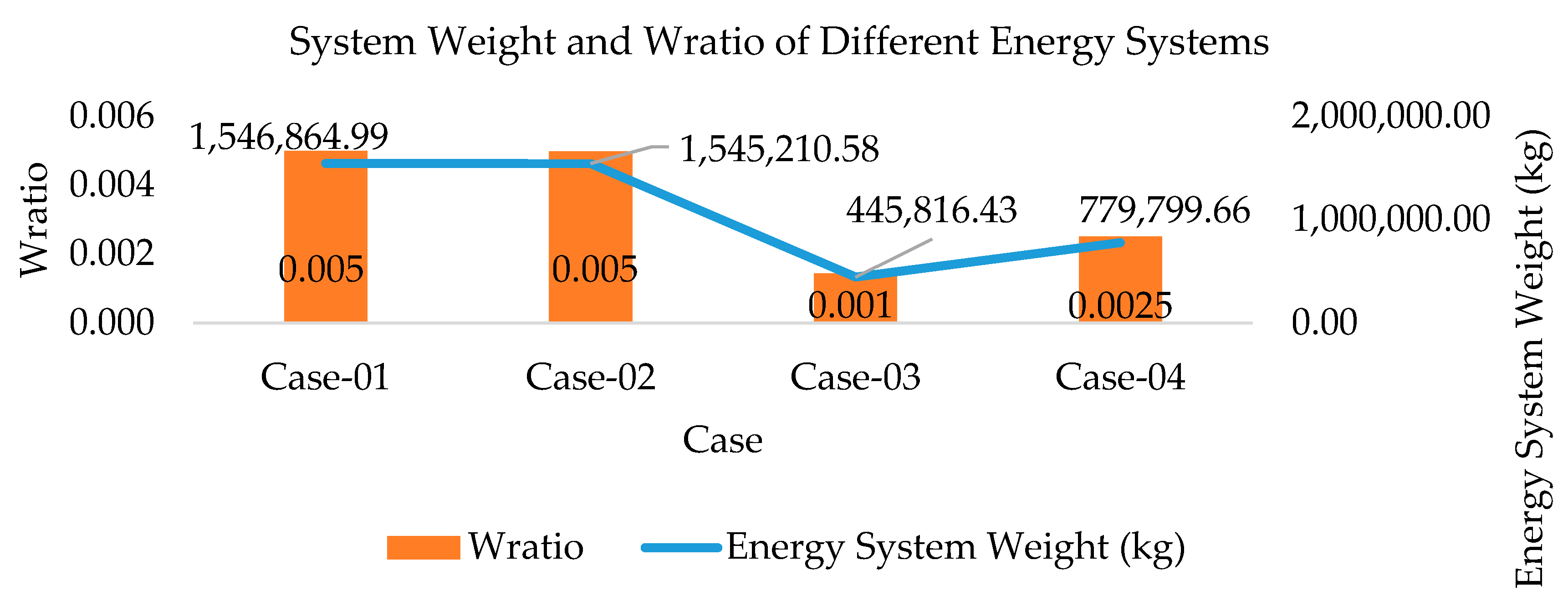
| Energy System Weight (kg) | 1,546,864.99 | 1,545,210.58 | 445,816.43 | 779,799.66 |
| LPSP | 0.080 | 0.079 | 0.080 | 0.08 |
| CO2 Emissions (ton/year) | 144,714.33 | 144,655.35 | 967.73 | 935.57 |
| Wratio | 0.005 | 0.005 | 0.001 | 0.0025 |
| GRF | 141.31 | 141.98 | 145.38 | 144.82 |
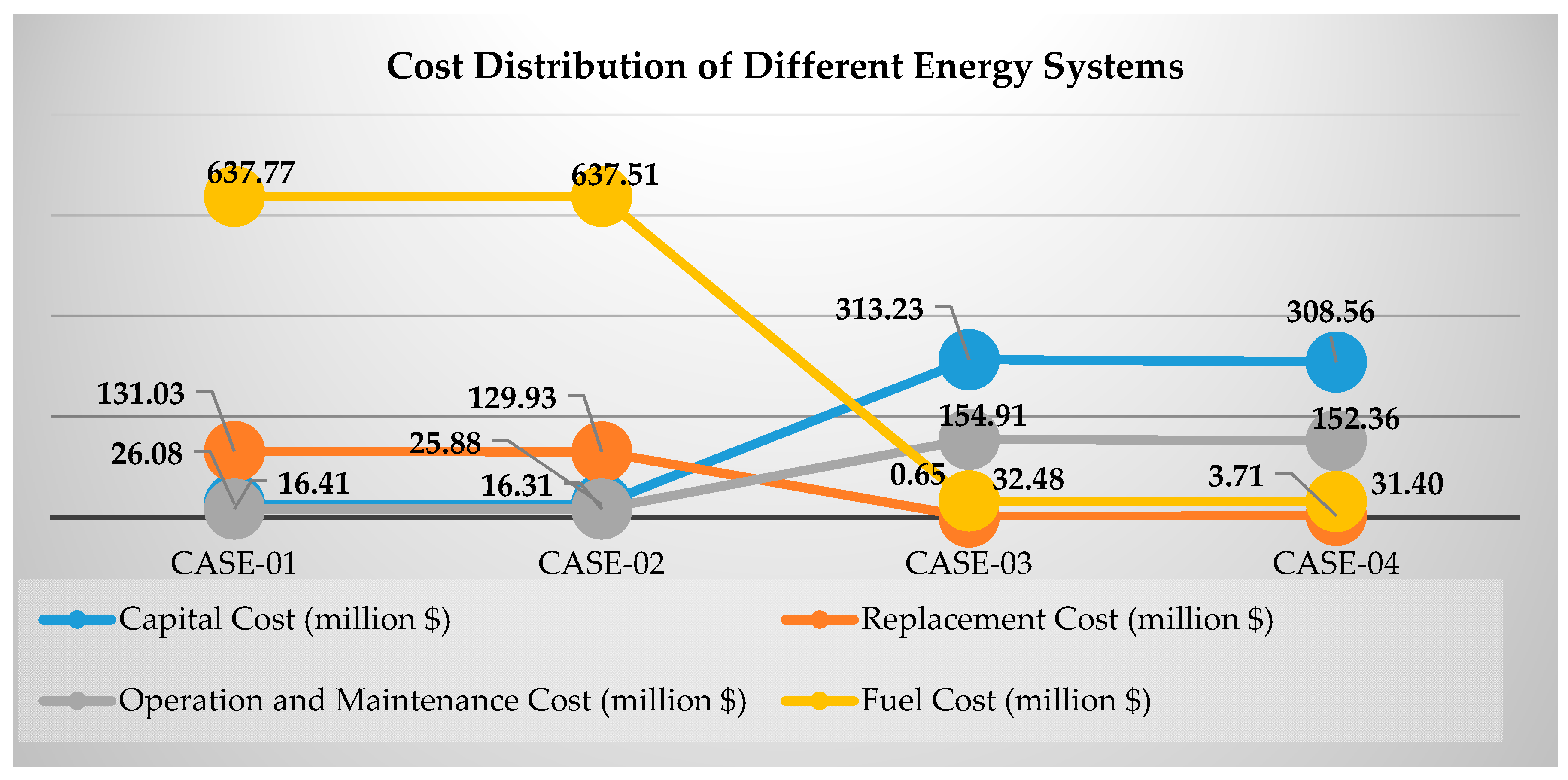
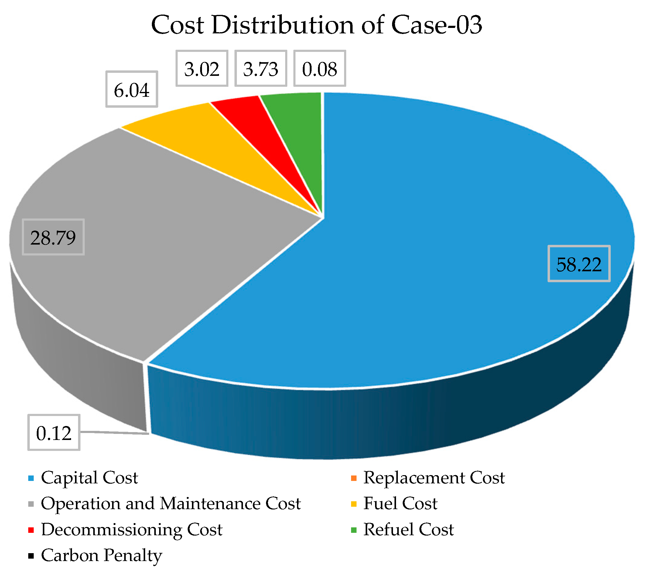
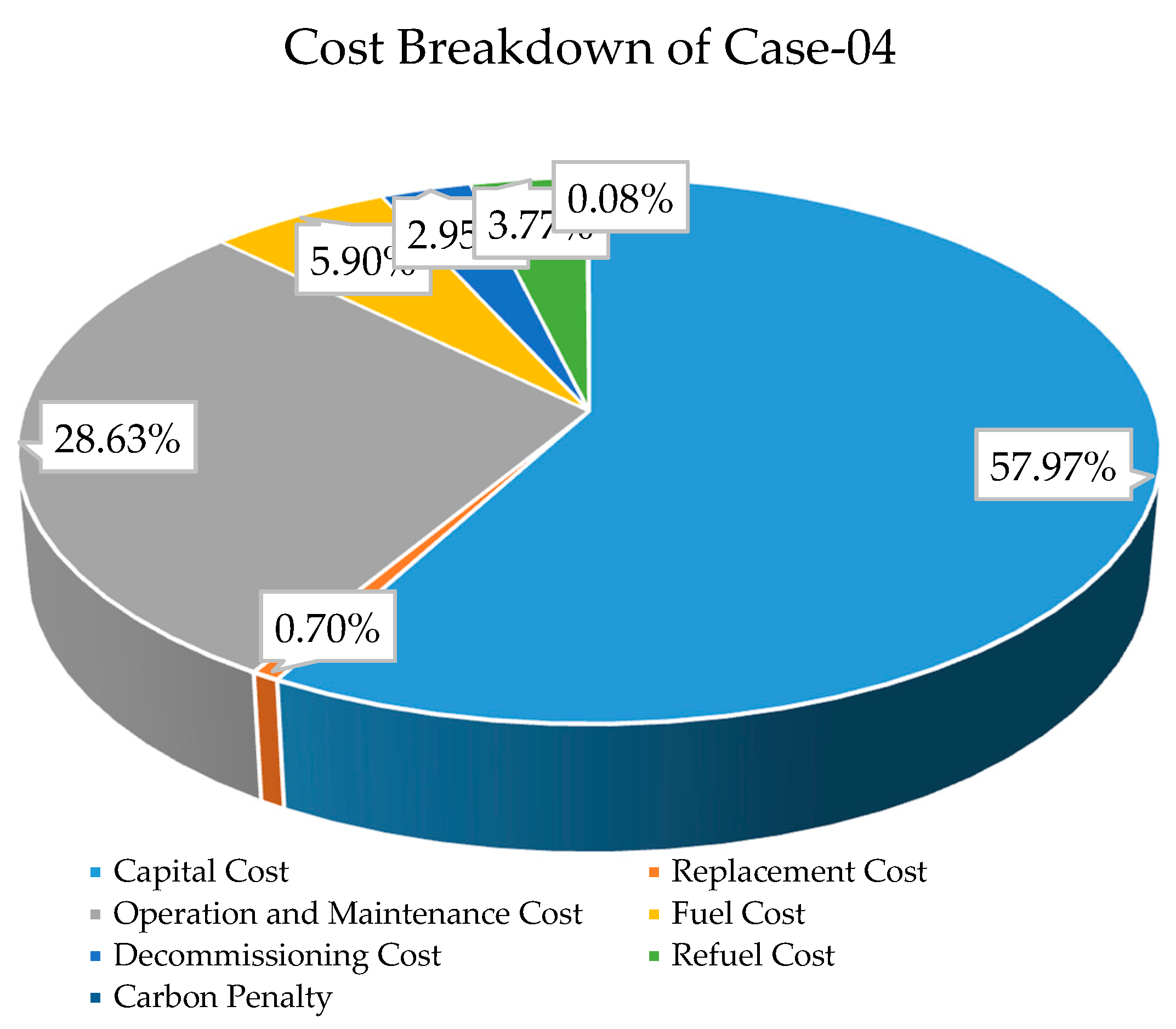
| Capital Cost ($) | 26,083,959.77 | 25,882,395.10 | 313,231,568.67 | 308,562,984.45 |
| Replacement Cost ($) | 131,028,335.96 | 129,934,105.16 | 651,048.07 | 3,710,762.34 |
| Operation and Maintenance Cost ($) | 16,414,843.54 | 16,310,161.71 | 154,912,891.56 | 152,358,576.04 |
| Fuel Cost ($) | 637,771,484.30 | 637,511,569.11 | 32,482,148.04 | 31,402,690.09 |
| Decommissioning Cost ($) | N/A | N/A | 16,241,074.02 | 15,701,345.05 |
| Refuel Cost ($) | N/A | N/A | 20,087,311.63 | 20,087,311.63 |
| Carbon Penalty ($) | 66,302,976.09 | 66,275,955.20 | 443,381.32 | 428,646.72 |
| Salvage Value ($) | 0.00 | 10,324.12 | 0.00 | 140,134.20 |
Publisher’s Note: MDPI stays neutral with regard to jurisdictional claims in published maps and institutional affiliations. |
© 2021 by the authors. Licensee MDPI, Basel, Switzerland. This article is an open access article distributed under the terms and conditions of the Creative Commons Attribution (CC BY) license (https://creativecommons.org/licenses/by/4.0/).
Share and Cite
Gabbar, H.A.; Adham, M.I.; Abdussami, M.R. Optimal Planning of Integrated Nuclear-Renewable Energy System for Marine Ships Using Artificial Intelligence Algorithm. Energies 2021, 14, 3188. https://doi.org/10.3390/en14113188
Gabbar HA, Adham MI, Abdussami MR. Optimal Planning of Integrated Nuclear-Renewable Energy System for Marine Ships Using Artificial Intelligence Algorithm. Energies. 2021; 14(11):3188. https://doi.org/10.3390/en14113188
Chicago/Turabian StyleGabbar, Hossam A., Md. Ibrahim Adham, and Muhammad R. Abdussami. 2021. "Optimal Planning of Integrated Nuclear-Renewable Energy System for Marine Ships Using Artificial Intelligence Algorithm" Energies 14, no. 11: 3188. https://doi.org/10.3390/en14113188
APA StyleGabbar, H. A., Adham, M. I., & Abdussami, M. R. (2021). Optimal Planning of Integrated Nuclear-Renewable Energy System for Marine Ships Using Artificial Intelligence Algorithm. Energies, 14(11), 3188. https://doi.org/10.3390/en14113188