Improvement Dependability of Offshore Horizontal-Axis Wind Turbines by Applying New Mathematical Methods for Calculation the Excess Speed in Case of Wind Gusts

Abstract

The problem of increasing the reliability of wind turbines exists in the development of new offshore oil and natural gas fields. Reducing emergency situations is necessary due to the autonomous operation of drilling rigs and bulk seaports in the subarctic and Arctic climate. The relevance of the topic is linked with the development of a methodology for theoretical and practical studies of gas dynamics when gas flows in a pipe, based on a mathematical model using new mathematical methods for calculation of excess speeds in case of wind gusts. Problems in the operation of offshore wind turbines arise with storm gusts of wind, which is comparable to the wave movement of the gas flow. Thus, the scientific problem of increasing the reliability of wind turbines in conditions of strong wind gusts is solved. The authors indicate a gross error in the calculations when approximating through the use of the Fourier series. The obtained results will allow us to solve one of the essential problems of modeling at this stage of its development, namely: to reduce the calculation time and the adequacy of the model built for similar installations and devices. Experimental studies of gas-dynamic flows are carried out on the example of a physical model of a wind turbine. In addition, a computer simulation of the gas-dynamic flow process was carried out. The use of new approximation schemes in processing the results of experiments and computer simulation can reduce the calculation error by 1.2 percent.

1. Introduction

1.1. Relevance of the Research Topic

At present, a reliable autonomous energy supply is an urgent practical task for oil and gas bulk seaports located in the arctic and subarctic climates. This applies to the industrial part of drilling rigs. It should be noted that the development of new marine and coastal fields is impossible without the construction of heat and electricity sources. Since the newly developed fields are located at a considerable distance from the centralized power grids. The source of electricity supply can be a renewable energy source, for example, wind turbines.

1.2. Solving a Scientific Problem

The use of offshore wind turbines is becoming increasingly common in the European Union. It should be noted that the most optimal solution is deep water installations designed for higher wind speeds than coastal ones. However, this affects their reliability. First of all, this is due to storm gusts of wind, which in thermodynamics and gas dynamics is understood as wave fluctuations of the gas flow described by discontinuous gas-dynamic functions.

The solution of relevant problems in the field of gas dynamics is primarily based on the use of a mathematical description of the processes occurring in moving media. The development of new approximation methods can reduce the error and calculation time. Besides, when the mathematical modeling results are put into practice, the efficiency of devices increases due to gas flow parameters predicted more accurately.

Discontinuous gas-dynamic flows on offshore wind turbines occur during a storm. The current technologies allow you to turn off the installation itself when the wind speed exceeds the permissible speed. On the other hand, it is known that the higher the wind speed, the greater the power output of the wind turbine. In this paper, we propose a mathematical description of discontinuous gas-dynamic flows, which is made using new approximation methods. New mathematical models are needed to improve the reliability of offshore wind turbines, as well as to enable the wind turbine to operate in storm conditions, which will increase its efficiency.

1.3. Theoretical Purpose of the Developed Methodology

The actual problem of gas dynamics is the development of a new methodological approach to solve the problems of the gas dynamics of flows during their mathematical modeling and the use of difference schemes. The authors’ methods of approximating piece linear functions by recursive functions allow us to reduce the calculation error and avoid the appearance of the Gibbs effect.

When designing new technological devices, in which gas-dynamic flows are observed, it is necessary to carry out preliminary mathematical modeling of the running dynamic processes. To this end, the development of new approximation methods will significantly reduce the calculation time and the calculation error, which will allow us to perform more reliable mathematical modeling of gas-dynamic flows.

The new methodological approach to solving the problems of gas dynamics of flows during their mathematical modeling and the use of difference schemes allows us to increase the convergence of the initial and approximating functions, as well as to reduce the calculation error, without the Fourier series expansion and only through the use of standard trigonometric functions.

Besides, the applied new approximation methods fully correspond to the dynamic processes implemented in practice, which most fully solves the existing scientific problems in high-temperature engineering, gas flows, and wave disturbances in space.

1.4. Application of the Developed Methodology

It should be taken into account that discontinuous gas-dynamic flows occur in stormy conditions on offshore wind turbines. In this case, the wind speeds can significantly exceed the permissible ones in terms of the stability and reliability of the wind turbine. However, you can choose the operating modes of the wind turbine in stormy conditions, but only when building a mathematical model. The authors of the article have developed new approximation methods for discontinuous gas-dynamic functions, which allow us to describe the processes in storm conditions at offshore wind turbines with a sufficient degree of confidence.

In addition, the problem of improving the reliability of wind turbines is becoming more acute when developing new offshore oil and natural gas fields. This problem arises in connection with the autonomous operation of drilling rigs and bulk seaports in the subarctic and Arctic climate. The inability to use centralized energy supply systems leads to the use of renewable energy sources as the main sources of energy supply. In this regard, failures and emergencies at such power plants should be minimized. One of the ways to solve this problem is to optimize the operating modes of wind turbines in the event of strong wind gusts. The operation modes at supercritical speeds without an emergency shutdown must be worked out. The possibility of such work could be justified by applying new optimization methods, in particular, mathematical transformations associated with the approximation of piecewise linear functions.

1.5. Review of Scientific Investigations

The creation of a mathematical apparatus to describe the wind flow processes began in the first half of the 20th century. The very first models in the theory of gas dynamics are based on the Navier-Stokes condition [1] for the appearance of flows and are described by algebraic ratios. The Lanchester–Betz–Joukowsky model [2] is theoretically applicable for the coordinate system of a wind speed; it uses a one-dimensional stationary system of ordinary differential equations taking into energy and initial conditions. When integrating this system of equations, one can find a connection with the Navier--Stokes parameters beyond the wind speed. The speed of the wind can be taken into account through the use of simplified models, for example, the Acker and Hand model [3], or more complex ones with a detailed [4,5] and global [6,7] kinetic mechanism. All modern computer programs are based on mathematical three-dimensional models [8,9].

Modern studies in the areas dealing with wind speed [10] and the use of derivatives in the mathematical description of the process [11] are connected with the visualization of gas flows and increased accuracy of calculations. We should note the works of Zhen, Zhao, and Liu dealing with the gas flow problem [12]. The studies on the boundary layer during the gas flow [13] are also of much interest. Sheng and O’Connor carry out mathematical modeling of turbulent flows [14]. Similar works are performed by other researchers, including experimental studies [15,16,17,18,19,20,21,22,23].

The solutions proposed by the authors of the articles on the mathematical description of gas-dynamic flows allow us to solve certain problems of gas dynamics. However, these descriptions do not give a complete picture of the flow in the case of using functions with discontinuities, since in this case, the existing approximation methods give an error. It is necessary to develop approximation methods with a lower error, which will allow us to model discontinuous gas-dynamic flows in the event of a storm on offshore wind turbines.

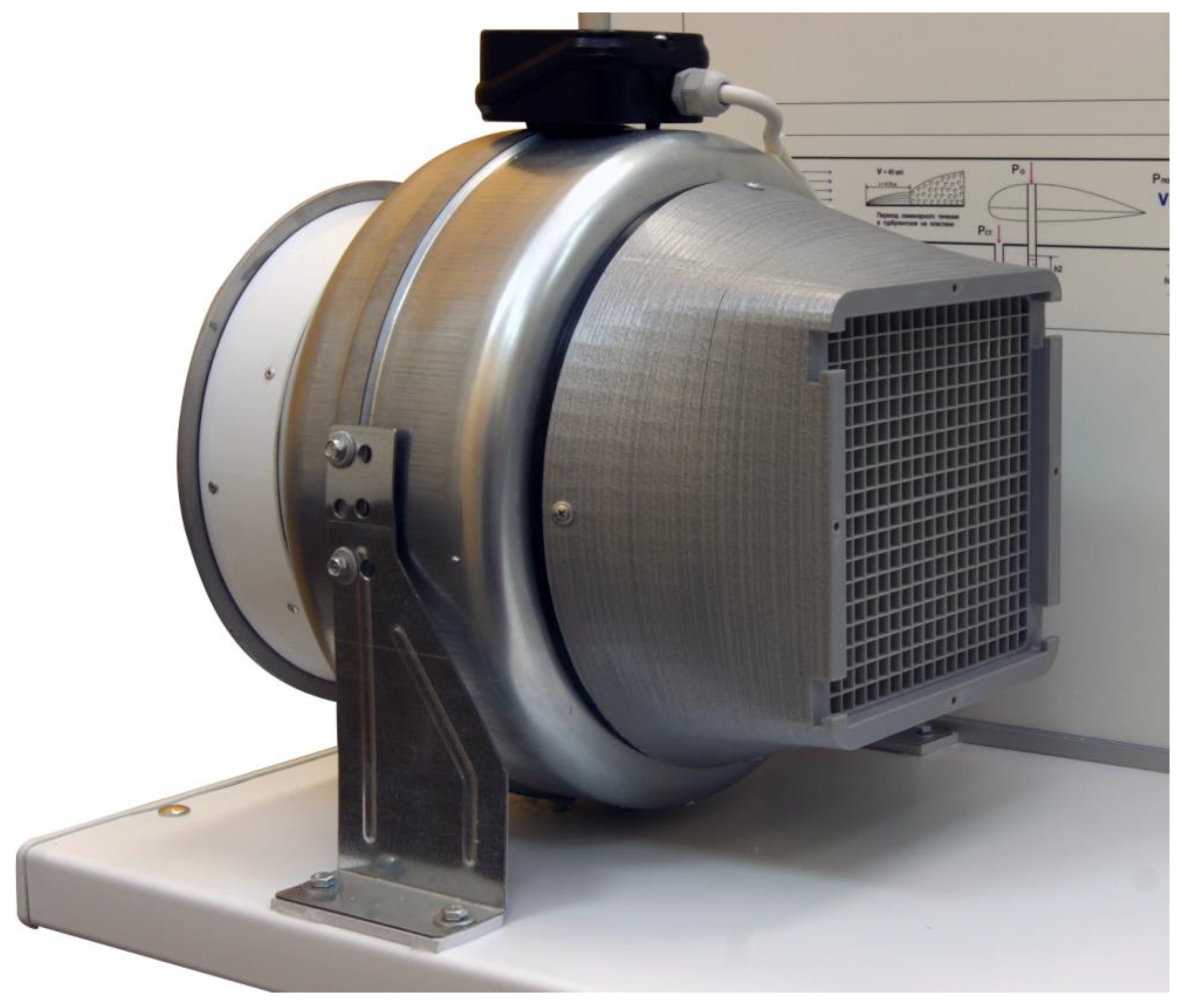
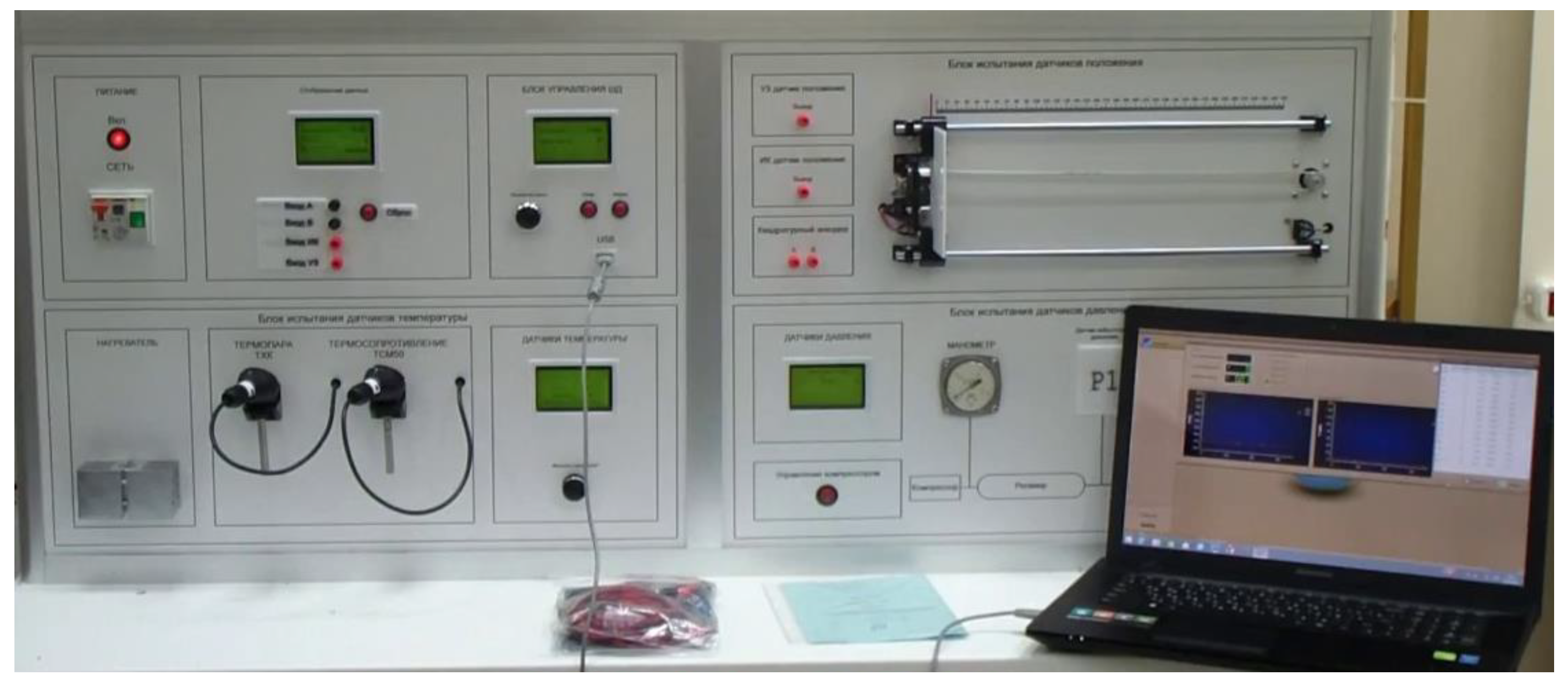
2. Experimental Unit

2.1. Experimental Investigations of Gas Dynamics of Air Flows

The experimental installation assumes the existence of a special channel for airflow and measuring devices. Figure 1 shows the movement of sensor tapes along the guide perpendicular to the channel.

The actual installation of the experimental setup is shown in Figure 2, Figure 3 and Figure 4.

Figure 2 shows a smaller copy of the wind turbine. This copy is functional to the same extent as the original. This installation is inserted into the wind tunnel in Figure 3.

The wind tunnel shown in Figure 3 is connected to secondary devices for visualizing the pressure drop (velocity) and temperature. These secondary devices are also displayed in special software on the laptop, Figure 4.

2.2. Reliability and Uncertainty of Measurement Device Data

The development of the experimental research methodology is based on the estimation of the uncertainty arising from each of its sources. The experimental installation is equipped with devices for measuring flow, temperature, and pressure. To determine the total uncertainty, you need to define each one separately, and then use the equations for the constructed model.

In the case of the authors’ research, the method itself contributes to the uncertainty, so this contribution can be expressed as a value that affects the final result. In this case, the uncertainty of the parameter is expressed directly in units of y, and the sensitivity coefficient ∂y/∂x = 1.

The result of the air velocity measurements—the arithmetic mean of 4.147 m/s is characterized by a standard deviation of 0.04 m/s. The standard uncertainty u(y) associated with precision under these conditions is 0.04 m/s. The model of this measurement, in this case, can be expressed by the equation y = (calculated result) + ε, where ε reflects all random effects under the given measurement conditions, with the sensitivity coefficient ∂y/∂x = 1.

The found uncertainty value is subject to revision only in the process of revalidation of the analysis methodology. Validation of the measurement method was carried out during repeated tests of the boiler unit in the conditions of operation at the oil and gas field in the far north. To ensure that the performance indicators obtained during the development of the methodology are achieved with its specific application, the methodology is validated. In the case of the author’s research, the technique was conducted in an interlaboratory study, which resulted in additional data on the effectiveness.

Similarly, the uncertainty of other variables, such as temperature and pressure, was evaluated. The calculated value of the correction introduced in the measurement result, necessary to take into account the influence of the heat sink on the thermometer body and the thermal resistance between the sensor element of the thermometer and the channel wall, is 0.025 °C. The uncertainty of the correction value using thermal modeling lies in the range from 0.005 to minus 0.005 °C. There are reasons to assume that the probability density of uncertainty has a uniform distribution. The certificate of verification of the used measuring device indicates its confidence error is equal to 0.01 °C with a probability of 0.95 (2σ).

The calculated value of the correction introduced into the measurement result, which is necessary to account for the influence between the pressure gauge sensor element and the channel wall, is 0.05 MPa. The uncertainty of the correction value using thermal modeling lies in the range from 0.01 to minus 0.01 MPa. There are reasons to assume that the probability density of uncertainty has a uniform distribution. The certificate of verification of the used measuring device indicates its confidence error equal to 0.02 MPa with the probability of 0.95 (2σ).

Thus, we consider the case of direct measurements, which does not require the representation of the measured value in the form of functional dependence. In this case, the uncertainty of the measurement result can be represented as the sum of the uncertainties caused by the influence of various factors, which can be determined based on all available information. At the same time, it can be assumed that all the components of uncertainty are not correlated.

3. Mathematical Part

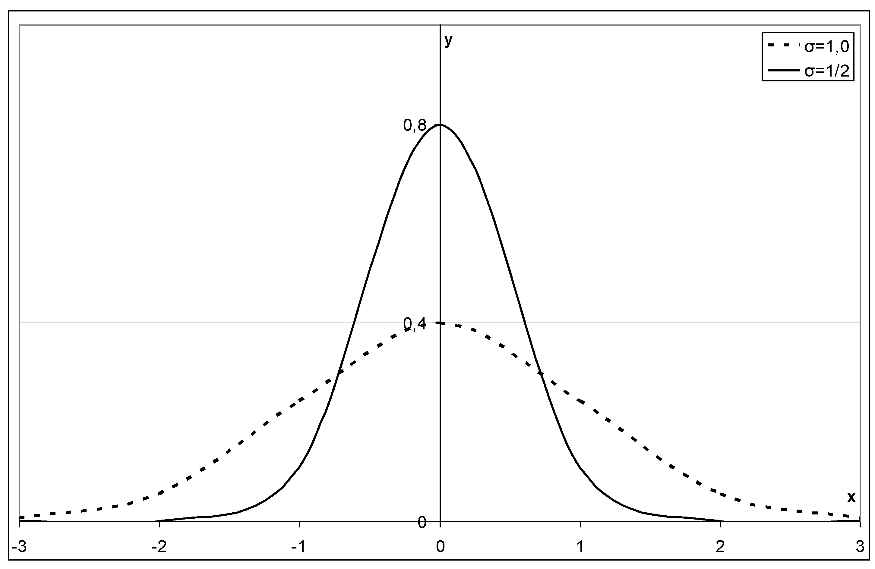
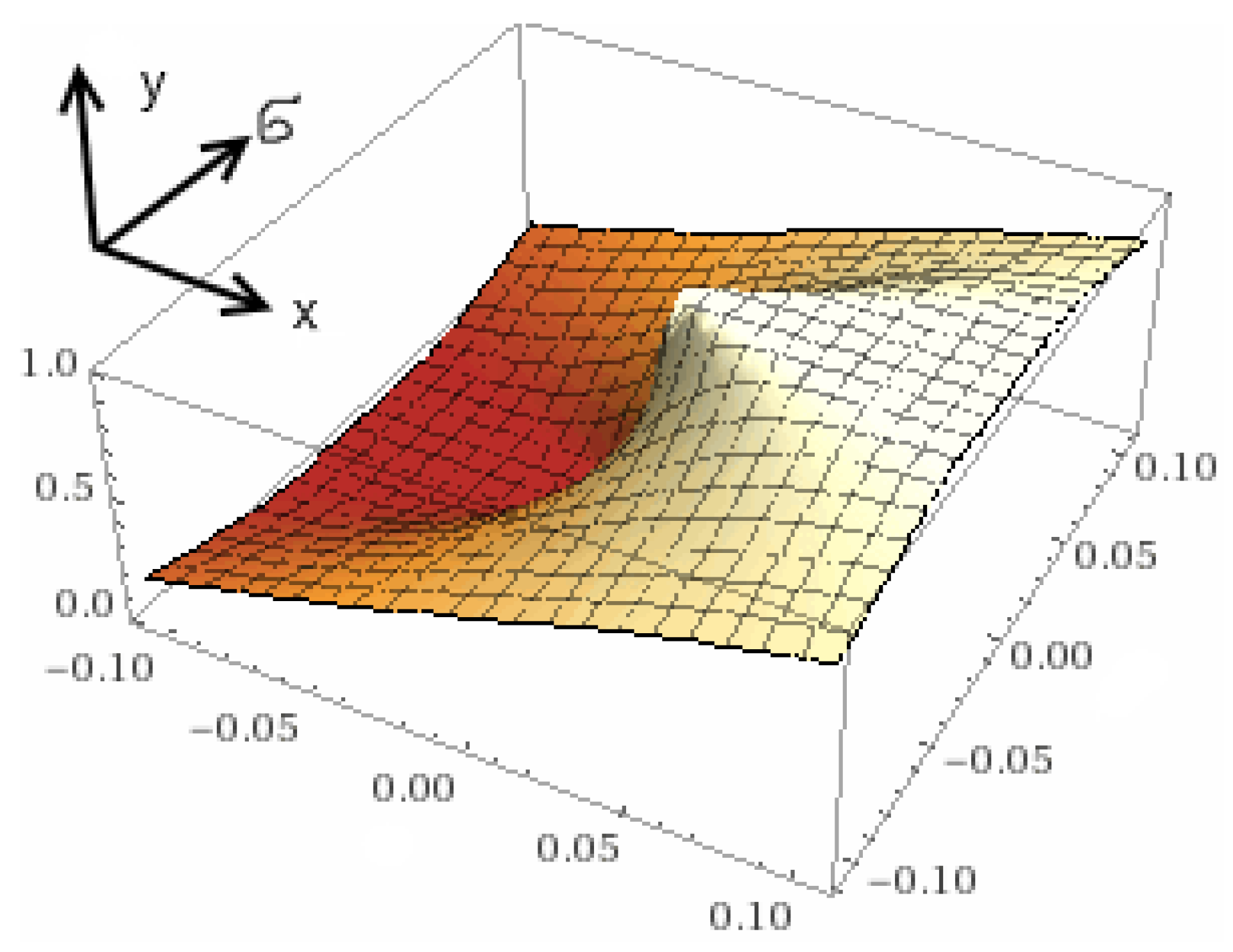
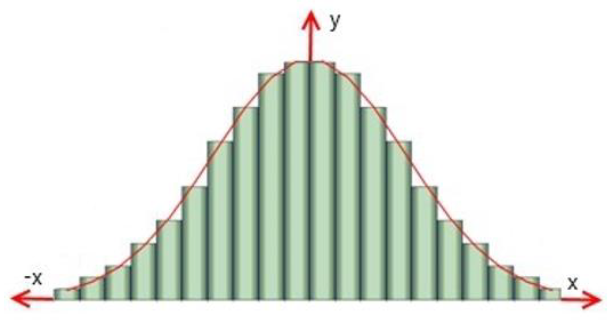
3.1. Application of the Normal Probability Distribution of Wind Velocity Deviation from the Mean Value

The deviation of the wind speed can be described in the range of characteristic speeds ω, in this case, the intervals should be taken F(ω₁/ω₂) and F(ω₂/ω₃). In this case, we obtain:

$$F_i=0.5·\left[F\left({\mathsf{\omega }}_1/{\mathsf{\omega }}_2\right)+F\left({\mathsf{\omega }}_2/{\mathsf{\omega }}_3\right)\right]$$

(1)

When determining the deviation according to Equation (1), specific points are formed F_i. The specific points obtained in this way form a continuous curve, which characterizes the ensemble of velocities. Given the continuity of the velocity curve, it can be differentiated or integrated to describe in detail the process of displacement of velocity vectors in wind gusts, and later to build a mathematical model of the reliability process in storm conditions. The reliability of the decision should be increased with an increase in the number of direct laboratory measurements.

Further, taking into account the transition to a continuous function and the mandatory increase in the number of measurements, as well as analyzing the fundamental foundations of the theory of distribution, we can conclude that the Gaussian curve corresponds to the chosen type of function. In addition, the density of the normal probability distribution of deviation from the mean value, which is denoted by $\theta \left(u\right)$, define it by the standard equation:

$$\theta \left(u\right)=exp\left(-0.5·u^2\right)/{\left(2·\pi \right)}^{0.5}$$

(2)

In Equation (2), the function argument is u—this is the standard normal deviation:

$$u=\frac{\delta -\xi }{\xi ·\sigma }$$

(3)

In the Equation (3) ξ—the value that corresponds to the speed ω, corresponding to the maximum on the considered curve F_i, σ—standard of deviation, and σ²—dispersion.

Placing near the maximum ξ the ensemble of velocities and reducing the values to a dimensionless form, we normalize the given function. While the definition of characteristics in the form of dependence on the standard of deviations σ allows one to standardize the function.

The error function obtained by (2) $\theta \left(u\right)$, which in this case is better called the deviation function, is tabulated. For the conditions of the problem presented in the article, the deviation function is shown in Figure 5. The standard deviation uniquely defines the function (2) and the values of u = 1 and u = −1 correspond to the inflection points on the curve constructed according to the dependence (2). Also according to the curve constructed in accordance with the fractional composition $\theta \left(u\right)$ the variance is easily determined σ² = (ω − ξ)²/(ξ·u)².

By determining the correlation coefficient between the practical results of the velocity deviation and the Gaussian curve in the usual way, we can quantify the reliability of the description (1). This technique can also be applied at the determination stage F(ω).

In addition, the authors emphasize that the developed method of normalization of the continuous function described by the Gaussian curve can be used to determine the density of the Gaussian distribution of a normalized quantity in 3D is shown in Figure 6, where it can be seen that the distribution is shifted to the region of positive values x.

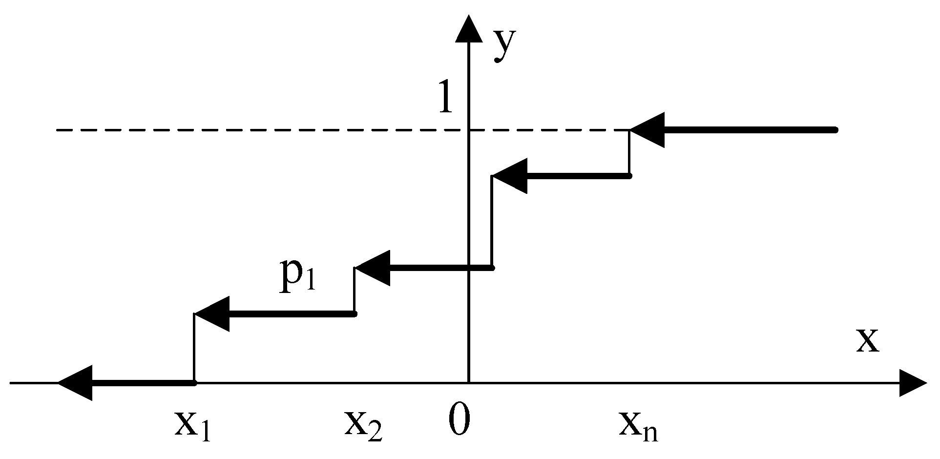
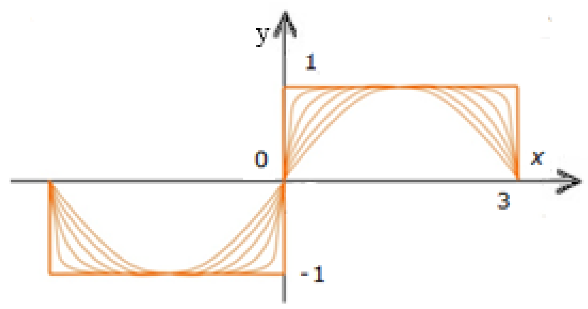
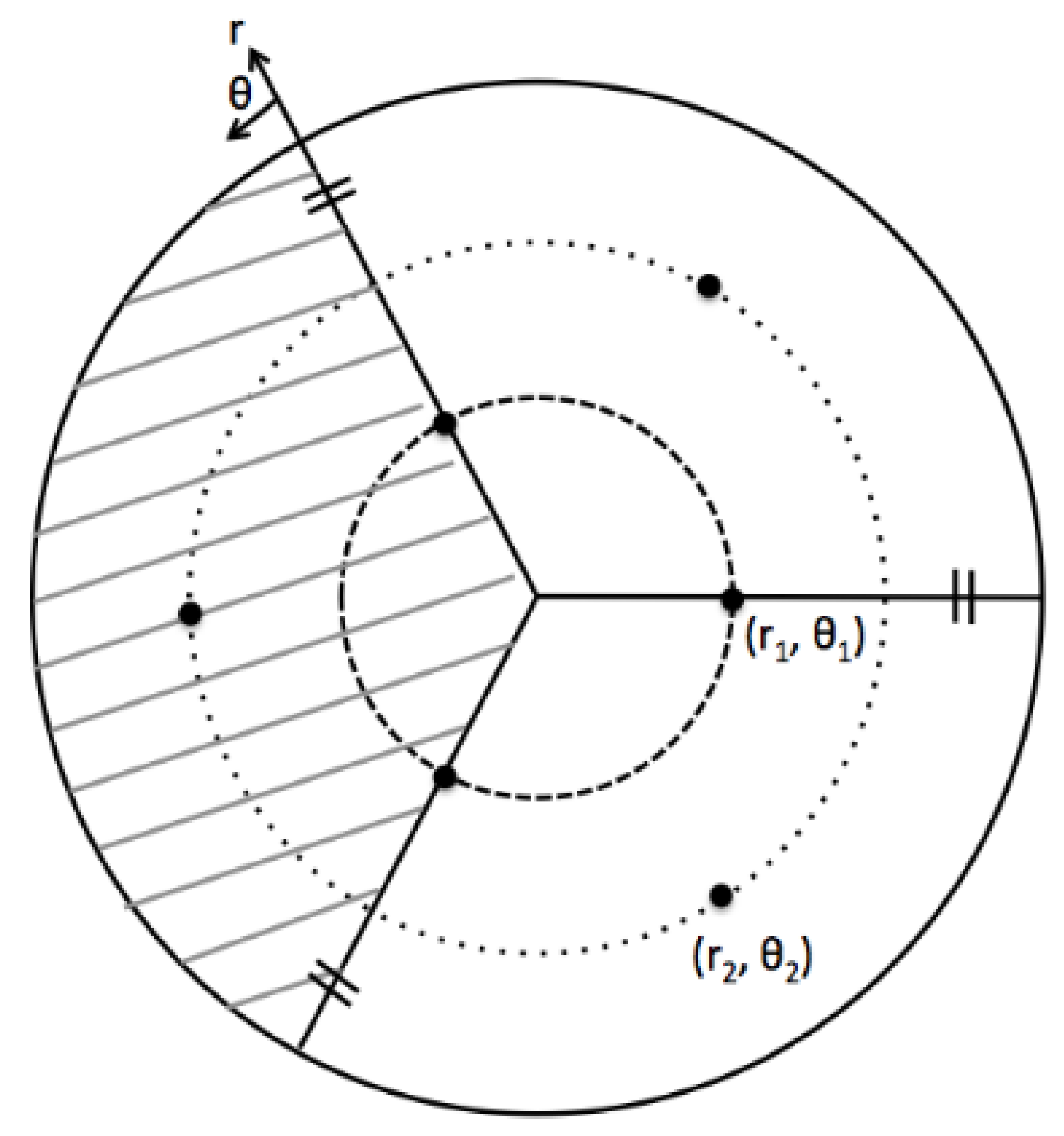
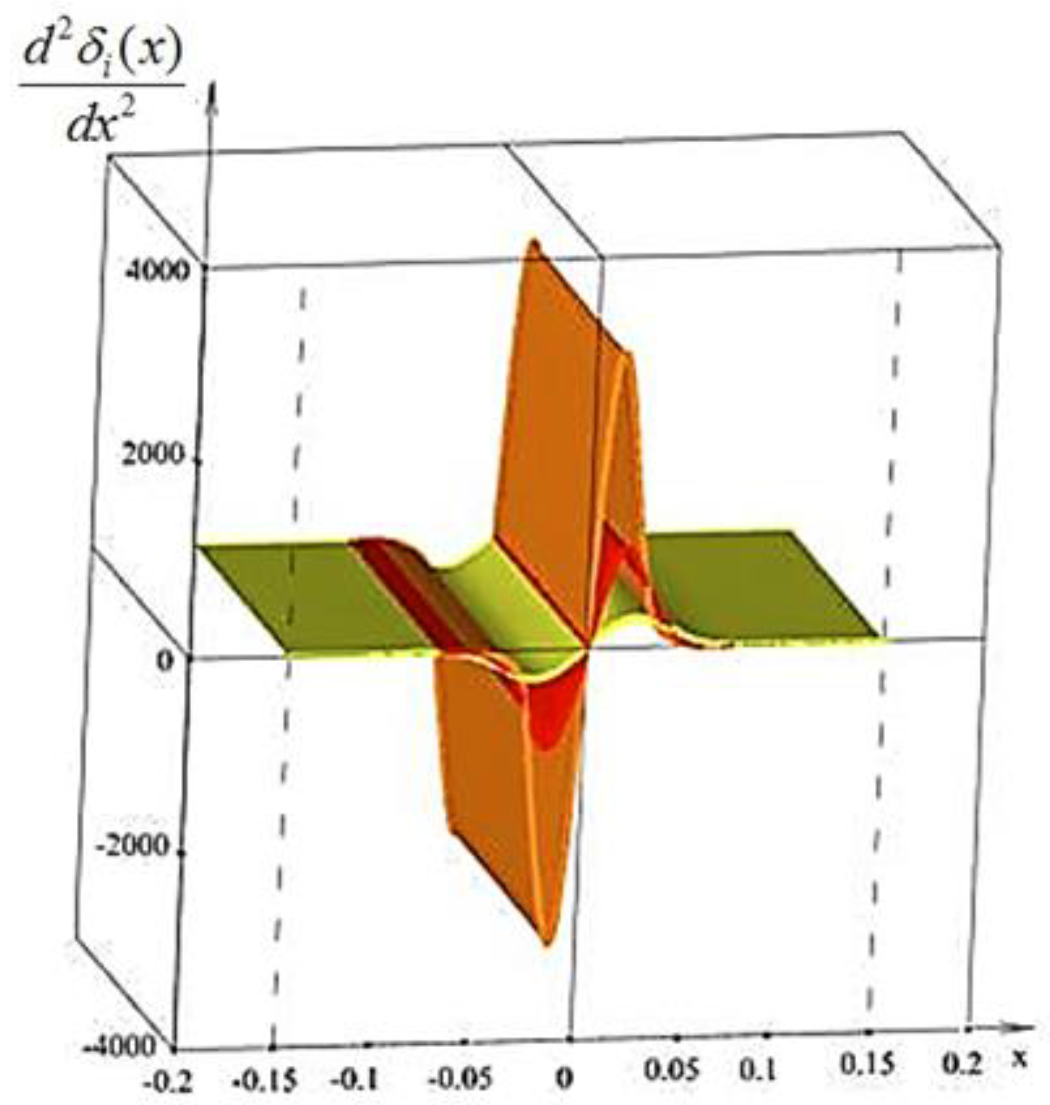
3.2. Approximation Methods. Application of Differential Curves to Describe the Velocity Distribution

For numerical simulation, the average speed value corresponding to the most frequently encountered speed value in a given system. This speed value can be found from the differential distribution curve, for the construction of which it is necessary to process the integral curve in Figure 5 by the method described above. At regular intervals of velocity changes Δω, which are chosen at random, build the ordinates up to the intersection with the integral curve, move these points to the ordinate axis, and find the value ΔG—differences between two adjacent ordinates. The number of segments Δω into which the abscissa is divided must be at least 8. Then, putting the values of the average velocities on the abscissa axis, and on the ordinate axis—ΔG/Δω, build rectangles, taking equal size intervals for the bases Δω, and for the height ΔG/Δω, Figure 7 and Figure 8.

3.3. Application of Piecewise Linear Functions and Recursive Function Approximations for the Mathematical Description of the Coal Dust Sieving Process

When solving this problem, the authors propose to take as a basis the resulting distribution graph—a step-like figure, Figure 8, which is described by a piecewise continuous function. Using the methods of the theory of linear systems, a solution can be obtained for each section of such a function. At the same time, problems often arise when constructing solutions for the entire domain of the definition of a piecewise linear function, linking solutions for sections with the need to use special mathematical methods. To simplify calculations, working with piecewise linear functions, in many cases, approximation methods are applied. One of the most widely used methods for approximating piecewise linear functions is to decompose these functions using Fourier series:

$$y={\displaystyle \sum }_{i=1}^{\infty }{p}_i·{\phi }_i$$

(4)

In the Equation (8) $\left\{{\phi }_1,{\phi }_2,\dots ,{\phi }_n,\dots \right\}$—an orthogonal system in a functional Hilbert space L₂[−π, π] measurable functions with Lebesgue integrable squares:

$$y\in L_2\left[-\pi ,\pi \right],p_i=\frac{\left(y·{\phi }_i\right)}{{\phi }_i{}^2}$$

(5)

As an orthogonal system, the trigonometric system is often taken 2π—periodic functions $\left\{1,sin nx, cosnx;n\in N\right\}$.

The use of the Fourier series has disadvantages. For example, with a relatively small number of terms in the Fourier series used to decompose a piecewise linear function, the approximating function has a pronounced wave-like character even within a single rectilinear section of the piecewise linear function, which leads to a sufficiently large approximation error. In the work of Professor S. V. Aliukov, it is shown that for a function with rectangular pulses

$$y_0\left(x\right)=sign\left(sinx\right)$$

(6)

point x = π/m, m = 2[(n + 1)/2] and [(n + 1)/2]—integer part of a number (n + 1)/2, is the maximum point of the partial sum $S_n\left(f_0\right)$ of the trigonometric Fourier series, and

$$S_n{\left(y_0,\frac{\pi }{m}\right)}_{n\to \infty }\to \frac{2}{\pi }\underset{0}{\overset{\pi }{{\displaystyle \int }}}\frac{sint}{t}dt\approx 1.17898$$

(7)

That is, the value of the absolute error will be equal to:

$$\left|y_0\left(\pi /m\right)-\underset{n\to \infty }{\lim }{S}_n\left(y_0, \pi /m\right)\right|>0.178$$

(8)

Then the relative error is more than 17% regardless of the number of terms in the partial sum of the Fourier series.

In addition, for the graph of the approximating function, an increased approximation error appears in the vicinity of the discontinuity points of the original function. This manifests the so-called Gibbs effect, and with an increase in the number of harmonics, the Gibbs effect does not disappear, which leads to extremely negative consequences of using the approximating function.

New approaches to the approximation of piecewise linear functions.

To eliminate these shortcomings, it is proposed to approximate the original step function with a sequence of recursive periodic functions:

$$\left\{y_n\left(x\right)|y_n\left(x\right)=sin\left(\left(\frac{\pi }{2}\right)·y_{n-1}\left(x\right)\right), y_1\left(x\right)=sinx;n-1\in N\right\}\subset C^{\infty }\left[-\pi ,\pi \right]$$

(9)

The approximation (9) is based on the use of trigonometric expressions, but not in the form of summands, as in the Fourier series, but in the form of embeddings.

The graphs of the step function (9) and its four successive approximations in this case have the form (Figure 9).

It should be noted that even with relatively small values of n when using the procedure (9), the graph of the approximating function approximates the original function y quite well. In the case of the proposed approximation method, the sinusoid is stretched along the rectilinear sections of the graph of the original function. At the same time, no fluctuations of the approximating function occur within the rectilinear sections of the original step function. The Gibbs effect is also completely absent.

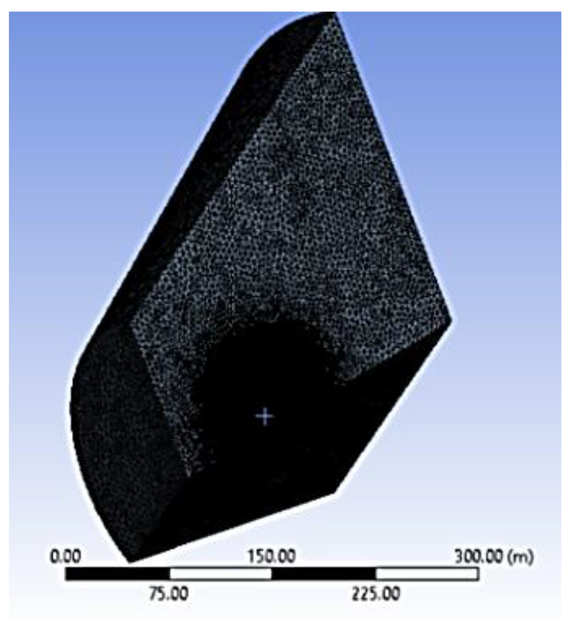
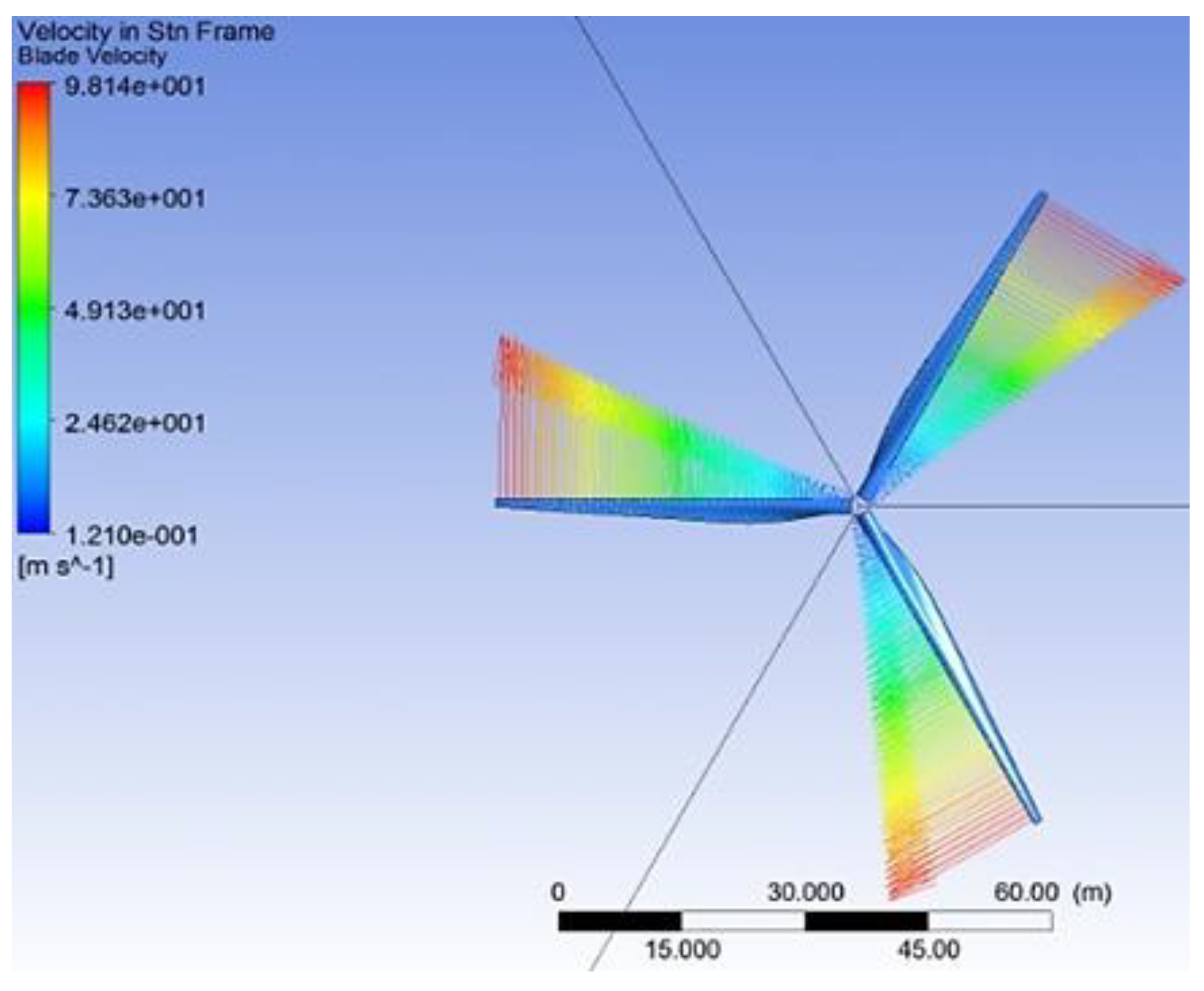
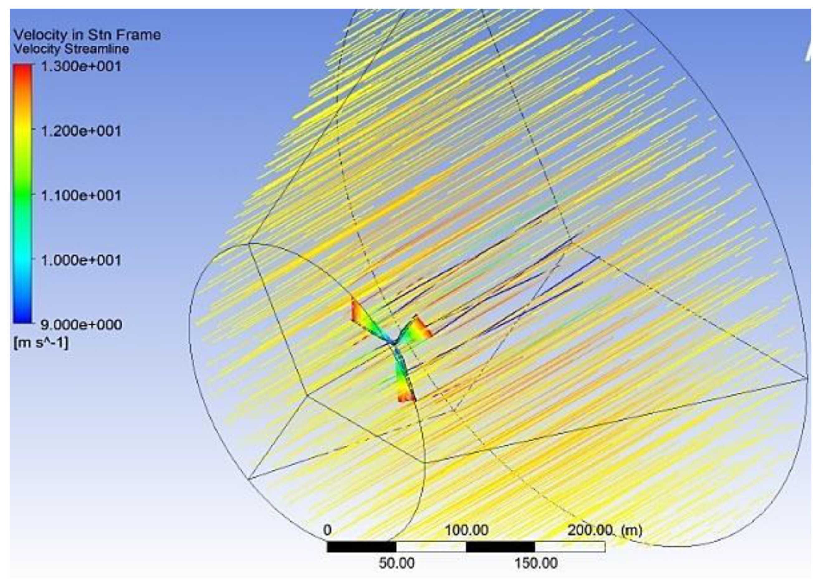
3.4. Computer Modeling of the Gas Dynamics of Air Flow

The authors emphasize that the obtained results of the mathematical description can be applied to gas-dynamic flows, for example, in the ANSYS CFD computer environment, which will lead to increased stability and convergence of the calculations. As mentioned earlier, the error of the proposed calculation method based on the use of approximating functions instead of the Fourier series makes the theoretical calculation more correlated to the results obtained by other known methods. Besides, the error during mathematical modeling is reduced due to the use of specific grids and models applied only for the flow of homogeneous gases.

When solving problems of gas dynamics, especially for wind turbines, it is necessary to take into account the existing experience of modeling. However, when using new approximation methods for discontinuous gas-dynamic flows, it is necessary to focus on wind speeds that occur in stormy conditions at offshore wind turbines.

Besides, we will present recommendations for the further use and expansion of the application range of the results obtained during computer modeling of gas dynamics processes. The main functions of the parameters for k-omega computer mathematical modeling, for example, in ANSYS CFD airflow, can be approximated using the authors’ findings.

The turbulent wind flows towards the negative z-direction at 12 m/s, which is a typically rated wind speed for a turbine this size. This incoming flow is assumed to make the blade rotate at an angular velocity of −2.22 rad/s about the z-axis (the blade is thus spinning clockwise when looking at it from the front, like most real wind turbines). The tip speed ratio (TSR) (the ratio of the blade tip velocity to the incoming wind velocity) is therefore equal to 8 which is a reasonable value for a large wind turbine. Note that to represent the blade being connected to a hub, the blade root is offset from the axis of rotation by 1 m. The hub is not included in our model.

Governing Equations

The governing equations are the continuity and Navier–Stokes equations. These equations are written in a frame of reference rotating with the blade. This has the advantage of making our simulation not require a moving mesh to account for the rotation of the blade. The equations that we will use look as follows:

Conservation of mass:

$$\frac{\partial \rho }{\sigma t}+\nabla \rho {\upsilon }_2=0$$

(10)

Conservation of Momentum (Navier-Stokes):

$$\nabla (\rho {\upsilon }_r {\upsilon }_r)+\rho (2\varpi \times {\upsilon }_r+\varpi \times \varpi \times r)=-\nabla p+\nabla \overline{T}r$$

(11)

where v_r is the relative velocity (the velocity viewed from the moving frame) and ϖ is the angular velocity.

Note the additional terms for the Coriolis force (2ϖ × v_r) and the centripetal acceleration (ϖ × ϖ × r) in the Navier–Stokes equations. In Fluent, we’ll turn on the additional terms for a moving frame of reference and input ϖ = −2.22 rad/sec. Important: we use the Reynolds Averaged form of continuity and momentum and use the SST k-omega turbulence model to close the equation set.

Boundary Conditions

We model only 1/3 of the full domain using periodicity assumptions Figure 10:

$$\overrightarrow{\upsilon }(r_1,\theta )=\overrightarrow{\upsilon }(r_1,{\theta }_1-{120}^{°}n)$$

$$\{\begin{array}{l}\overrightarrow{\upsilon }(r_1,\theta )=\overrightarrow{\upsilon }(r_1,{\theta }_1-{120}^{°}n), for n=1,2,3,\dots \\ =\overrightarrow{\upsilon }(r_1,{240}^{°}-{120}^{°}(1))=\overrightarrow{\upsilon }(r_1,{120}^{°})=\\ =\overrightarrow{\upsilon }(r_1,{240}^{°}-{120}^{°}(2))=\overrightarrow{\upsilon }(r_1,0^{°});\\ \overrightarrow{\upsilon }(r_2,\theta )=\overrightarrow{\upsilon }(r_2,{\theta }_2-{120}^{°}n), for n=1,2,3,\dots \\ =\overrightarrow{\upsilon }(r_2,{180}^{°}-{120}^{°}(1))=\overrightarrow{\upsilon }(r_2,{60}^{°}).\end{array}$$

(12)

Therefore this proves the velocity distribution at theta of 0 and 120 degrees are the same. If we denote theta_1 to represent one of the periodic boundaries for the 1/3 domain and theta-2 being the other boundary, then

$$\overrightarrow{\mathrm{v}}\left(r_i{,\mathsf{\theta }}_1\right) =\overrightarrow{\mathrm{v}}\left(r_i{,\mathsf{\theta }}_2\right)$$

(13)

$$\mathrm{v}\left(r_i{,\mathsf{\theta }}_1\right) = \mathrm{v}\left(r_i{,\mathsf{\theta }}_2\right)$$

(14)

the boundary conditions on the fluid domain are as follow:

Inlet: Velocity of 12 m/s with a turbulent intensity of 5% and turbulent viscosity ratio of 10, Outlet: Pressure of 1 atm, Blade: No-slip, Side Boundaries: Periodic.

Numerical Solution Procedure in ANSYS

FLUENT converts these differential equations into a set of algebraic equations. Inverting these algebraic equations gives the value of (u, v, w, p, k, and omega) at the cell centers. Everything else is derived from the cell centers’ values (post-processing). In our mesh, we’ll have around 10,000,000 cells. The total number of unknowns and hence algebraic equations is 10,000,000 × 6 = 60 million.

This huge set of algebraic equations is inverted through an iterative process. The matrix to be inverted is huge but sparse. In FLUENT, we will use the pressure-based solver.

Hand-Calculations of expected results

According to the specification sheet of the turbine GE 1.5 xle wind, one simple hand calculation that we can do now before even starting our simulation is to find theoretical wind velocity at the tip. We can then later compare our answer with what we get from our simulation to verify that they agree. The velocity (v), on the blade, should follow the equation:

$$\upsilon =r\cdot \varpi$$

(15)

Plugging in our angular velocity of 2.22 rad/s and using the blade length of 43.2 m plus 1 m to account for the distance from the root to the hub, we get 44.2 m,

$$\upsilon =2.22\times 44.2=98.12 \mathrm{m}/\mathrm{s}.$$

Additionally, by using the simple one-dimensional momentum theory, we can estimate the power coefficient which is the fraction of harnessed power to total power in the wind for the given turbine swept area. This analysis uses the following assumptions:

The flow is steady, homogenous, and incompressible.

There is no frictional drag.

There is an infinite number of blades.

There is a uniform thrust over the disc or rotor area.

The wake is non-rotating.

The static pressure far upstream and downstream of the rotor is equal to the undisturbed ambient pressure.

According to this blade is meant to resemble GE 1.5 xle wind turbine blade. The specification sheet of this turbine states the rated power of this turbine to be 1.5 MW, the rated wind speed to be 11.5 m/s, and the rotor diameter to be 82.5 m. A power and power coefficient [9] is then defined as

$$P=T\cdot \omega$$

(16)

$$C_p=\frac{P_{rated}}{P_{wind}}=\frac{P_{rated}}{0.5\rho A{V}_{rated}^3}$$

(17)

$$C_p=\frac{1,500,000}{0.5\times 1.225\times \left(\frac{\pi \left({82.5}^2\right)}{4}\right)\times \left({11.5}^3\right)}=0.3$$

The resulting power coefficient of 0.3 is very reasonable. We will compare it to the power coefficient obtained from the simulation in the Verification and Conclusion section.

Hand-Calculations of expected results Betz equation and criterion

The Betz Equation deals with the wind speed upstream V_0 and the downstream V_3 wind speed of the turbine. The value of the Betz limit suggests that a wind turbine can be extracted at most 59.3 percent of energy in an undisturbed wind speed stream, it can be defined as:

Betz coefficient = Cp= 16/27 = 0.592593 = 59.3%

Power coefficient

The power generated by the kinetic energy of a free-flowing wind stream is shown in Figure 3, where is defined as the ratio of the power extracted by the wind turbine [relative to the energy available in the wind stream. Power coefficient (C_p), represented as extracted power over the total power, can be expressed by the induction factor (a) as

$${\mathrm{C}}_{\mathrm{p}}=4a{\left(1-a\right)}^2$$

(18)

where (a) is the induction factor, the fractional decrease in wind velocity between the free stream and rotor plane can be expressed in terms of an axial induction factor, a:

$$a=\frac{{\upsilon }_0-\upsilon }{{\upsilon }_0}$$

(19)

where, V is the velocity at the disk and it is defined by

$$\upsilon =\frac{1}{2}\left({\upsilon }_0+{\upsilon }_3\right)$$

(20)

v₀ and v₃ are free stream and downstream velocities, respectively. The amount of axial induction factor determines the amount of power extracted by the turbine.

Research method.

Geometry and Mesh generation.

In the following section, we will create our geometry and the blade volume from the fluid geometry. As we mentioned in the boundary condition part as showed in Figure 10. Periodicity assumptions.

Grid generation is often considered the most time-consuming part of CFD simulation. We start off by naming various faces of our geometry for later use in FLUENT and to make surface body referencing much easier when creating our mesh as shown in Figure 11.

Grid generation is often considered the most time-consuming part of CFD simulation. We start off by naming various faces of our geometry for later use in FLUENT and to make surface body referencing much easier when creating our mesh. After several attempts to mesh the geometry, we obtained a high-quality mesh of around 10,884,336 elements as shown in Figure 12.

This is considered very fine enough to obtain a sufficiently accurate solution. We are applying some global mesh settings that means that these settings will be applied to the whole mesh altogether. After applying controls to the whole mesh, we now apply mesh settings to specific areas of our geometry.

We will enable the visualization of a full 3-blade rotor. First, a hand calculation is based on the classical aerodynamic theory to find the theoretical wind velocity at the tip.

This data is comparing with the value of the velocity obtained by ANSYS. Figure 13 illustrates that the local wind turbine blade velocity is increasing with radius because of the rotation of the blades. The velocity of the tip, which is the highest velocity, is around 98.14 m/s, the same value as the equation.

The wind velocity streamline shows the velocity of the fluid domain around the three wind turbine blades as in Figure 14.

Note that the legend bar in the above picture presents color graduation from blue, which is the lowest velocity, until red. The inlet section has a yellow color so it is 12 m/s, as was mentioned earlier. The color blue in the streamlines means that when the airflow passes the blades so it is 10 m/s, it suffers a slowing down, and the velocity decreases. Clearly, an acceleration of the flow around the wake is represented by red color. All these features match the mass conservation and momentum theory.

3.5. Estimation of Errors in the Processing of Experimental Data and Computer Simulation Results

The smeared force and air velocity are defined by the integral of the distribution function of the deviation probability, and it is rational to set the integration limits from minus ∞ to the maximum air velocity corresponding to the upper limit of integration U

$$\Phi \left(\omega \right)=\frac{1}{\sigma \sqrt{2\pi }}{\displaystyle \underset{-\infty }{\overset{{\omega }_{max}}{\int }}exp\langle -0.5{\left[\left(\omega -\xi \right)/\left(\sigma \cdot \xi \right)\right]}^2\rangle }d\omega ={\Phi }_u\left(U\right)$$

(21)

Moreover, the normal distribution function Φ_i(U) is associated with the probability integral Φ(U) and the error function erf(U/2^0.5) by the dependence [24]

$${\Phi }_i\left(U\right)-1/2=0.5erf\left(U/\sqrt{2}\right)=\Phi \left(U\right)$$

(22)

Thus, the normal distribution function Φ_i(U) can be defined by the probability integral Φ(U) or by the error function erf(U/2^0.5), both dependencies are tabulated. But the practical adaptation of these dependencies has a number of features that are related to the reliability of the dependencies used. These features can be determined by the numerical analysis of the dependence (22) when changing the variability intervals of the arguments and their functions.

The numerical analysis shows that when the probability integral (21) is used for the range of positive and negative values u = (ω − ξ)/(ξ·σ), the difference between Φ(U) and Φ(ω) does not exceed 0.10% in the whole variation interval u. When calculating Φ_i(U) according to the dependence (22), the difference may exceed 10% in the range of negative values u, which is related to the lower limit of integration when obtaining the error function,

$$erf(U/2^{0.5})=\frac{2}{{\pi }^{0.5}}{\displaystyle \underset{0}{\overset{\mathsf{\pi }}{\int }}exp[-{(U/2^{0.5})}^2]}du$$

(23)

The resulting integral function is related to the known probability integral, which is given in tables in reference books; it makes it possible to calculate not only the total residue of the known distribution but also to define a number of properties of the smeared force.

Simulations were performed using the standard k-omega model. The authors also propose to use in the calculations the original version of the approximation of the generalized functions used in the simulation, which are derived from the delta function. In the standard k-omega model, the Gaussian is used in the calculation of smeared force f:

$$f^{\prime }=f_{AD}\otimes \left[\frac{{\epsilon }^{-1}}{{\pi }^{0.5}}exp\left[-{(D\cdot {\epsilon }^{-1})}^2\right]\right]$$

(24)

where ε = 3Δz, Δz is the reference grid size in the axis direction.

At the same time, the author of the paper, S.V. Aliukov, developed new methods of approximation of generalized functions.

The delta function is a derivative of the Heaviside function or the unit jump function, which is defined as

$$H(x)=\{\begin{array}{l}1, \forall x>0, \\ 0, \forall x>.\end{array}$$

(25)

Professor Aliukov suggested approximating the Heaviside function by a sequence of functions of the form

$$H_n\left(x)=0.5(1+f_n\right(x\left)\right)$$

(26)

where the sequence of recursive functions is determined by the relation

$$\left\{ f_n(x)|\begin{array}{l}{f}_n(x)=\sin \left((\pi /2)\cdot f_{n-1}(x)\right), \\ f_1(x)=\sin x; n-1\in N \end{array}\right\}\subset C^{\infty }[-\pi /2, \pi /2]$$

(27)

Finding the first derivatives of the Heaviside function approximations, we obtain successive approximations for the delta function.

As we approximated the generalized functions by analytic functions, we can differentiate these approximating functions and find their derivatives of any order. Thus, the main functions of the parameters for k-omega computer simulation of airflow can be approximated by the new method, not previously used in world practice. Figure 15 shows the approximation of the first and the second derivatives of the previously mentioned function.

The obtained approximations more accurately describe the original function. The suggestions for improving the mathematical apparatus of the standard k-omega model will help researchers to develop the theory of approximation by the recursive functions of Professor S.V. Aliukov. The results will solve one of the important problems of modeling at this stage of its development, namely reducing the calculation time and the suitability of the constructed model for similar installations and devices.

As a result, it was obtained that with the help of new methods of approximation and analysis of deviations of the airflow rate in the channel, it is possible to obtain more accurate results from experimental and numerical studies. In particular, the following is the 3D distribution of deviations in the calculation of air velocity.

The measurement results are affected by a large number of sources of small random errors. The whole set of measurements has a symmetric bell-shaped Gauss function as a limit distribution. The distribution center, which coincides with its maximum, will be the true value of the measured value. When using the method of approximation of Professor S.V. Aliukov, which is considered for the first time in relation to numerical methods of gas dynamics and experimental data for the flow of air in the aerodynamic channel.

4. Calculation of Measurement Uncertainty on a Laboratory Bench

The authors emphasize that the obtained modeling results in ANSYS are very akin to the theoretical and experimental data. The differences are insignificant since the error in the experimental measurements was leveled by the use of modern tools certified by the European Union. For example, this is evident by the temperature values. During standard modeling without the use of sampled data, the speed value ranged from 7.7–7.9 m/s. At the same time, when using the authors’ developments, the value of the average speed was 7.6 m/s. This value is the closest to the experimentally obtained values of 7.8 m/s. Thus, the maximum differences are obtained between the experimental data and computer modeling data without the use of the authors’ developments, while the maximum coincidence is shown between the average values according to the modeling results taking into account the sampled signals and the experiment. The error in calculating the results of scientific research is summarized in Figure 16.

We calculate the arithmetic mean of the wind speed from all measurements at a given point:

$$\mathsf{\omega }=\frac{1}{n}{\displaystyle \sum }_{i=1}^n{\omega }_i$$

(28)

After calculations using the Equation (28), we get the value ω = 7.84 m/s.

For sources of random uncertainty, we calculate the uncertainty by type A:

$$u_A\left(\omega \right)=\sqrt{\frac{{{\displaystyle \sum }}_{i=1}^n({\omega }_i-\omega )}{n\left(n-1\right)}}$$

(29)

Calculations using the Equation (29) gave the result $u_A\left(\omega \right)=0.8\%$.

For sources of systematic uncertainty (instrument error) calculating the uncertainty by type B:

$$u_B\left(\omega \right)=\frac{\Delta \omega }{\sqrt{3}}$$

(30)

Calculations using the Equation (30) showed the value of $u_B\left(\omega \right)=1.58\%$.

Calculate the total standard uncertainty:

$$u_C\left(\omega \right)=\sqrt{u_A{\left(\omega \right)}^2+u_B{\left(\omega \right)}^2}$$

(31)

Using the Equation (31), we get the value $u_C\left(\omega \right)=\sqrt{0.64+2.4964}=1.771\%$ For the confidence probability (coverage probability) P = 0.95 (recommended in the Uncertainty Calculation Guide), we set the coverage factor k = 2 and calculate the extended measurement uncertainty:

$$u=k{u}_C\left(\omega \right)$$

(32)

The total value of the extended uncertainty is determined to be u = 2∙1.771 = 3.542%. According to the regulatory document “Guidelines for measurements and their uncertainties in the countries of the Eurasian Economic Union”, the maximum permissible value is 5% for experimental data. Therefore, the results obtained fall within the confidence interval and confirm the data of modeling and experiments.

5. Sensitivity Analysis and Validation of Research Results

Validation of the methodology was carried out in the software package Matlab. Validation is shown on Figure 17 and Figure 18, with Error = 201.5694 (Normal), Error = 139.3117 (Lognormal). The graphs are made in Matlab.

Figure 17 and Figure 18 show the error value defined as Normal in Figure 17 and Lognormal in Figure 18. The values in these figures are dimensionless and represent: Error—error value, σ—sample variance, μ—sample expectation value.

In addition, it was assumed in [23] that the most basic functions can be used as the basis of the methodology. In the study [24], the direction of analysis laid down in [23] was partially continued. Finally, similar methods of thermodynamic analysis were used in [25,26,27].

6. Results and Discussion

The results of experimental studies allowed us to plot the speeds and showed dependence according to

Table 1. Dependence of measured speeds on channel width from deflection δ (by results of modeling).

Speed (u) m/s	11.2	11.4	11.7
Deviation (δ) m/s	0.02	0.05	0.09

.

The obtained results fit into the permissible measurement errors. Thus, the dependence of the airflow parameters on the mathematical model description is justified. The need for new methodological approaches to the theory of wind turbines is theoretically confirmed.

The results of the research are summarized in

Table 2. Dependence of speeds taking into account the experimental data and the mathematical approaches.

Speed (u) m/s	6.8	7.06	7.3
Deviation (δ) m/s	0.013	0.016	0.018

. Let’s compare the results taking into account experimental studies using new approximation methods at different airspeeds.

The authors emphasize that the obtained modeling results in ANSYS are very akin to the theoretical and experimental data. The differences are insignificant since the error in the experimental measurements was leveled by the use of modern tools certified by the European Union. The error in the mathematical modeling was reduced due to the use of the empirical data obtained by processing the signals from analogous equipment and subsequent sampling according to the technology developed by the authors. For example, this is evident by the velocity values u. During standard modeling without the use of sampled data, the velocity value ranged from 6.8–7.3 m/s, i.e., it averaged 7.05 m/s. At the same time, when using the authors’ developments, the value of the average velocity was 7.36 m/s. This value is the closest to the experimentally obtained values of 7.39 m/s. Thus, the maximum differences are obtained between the experimental data and computer modeling data without the use of the authors’ developments, while the maximum coincidence is shown between the average values according to the modeling results taking into account the sampled signals and the experiment.

The scientific developments of P.A.B. James, conducted relatively recently, show that the theory of gas dynamics of wind turbines has its drawbacks in relation to experimental studies. P.A.B. James and A.S. Bahaj presented the results of the research in the form of a developed model [6]. Researchers, for example, A. Sargsyan [7] and his colleagues proposed a hypothesis of the behavior of airflow in extreme conditions, and this hypothesis was partially confirmed by the developed mathematical model, which is consistent with the results of studies by P.A.B. James and A.S. Bahaj [6]. The hypotheses considered in the discussion were confirmed by the construction of mathematical models. These models fully correspond to each other, as well as to the basic physical laws, in particular, the equations of conservation of mass and energy, as well as the boundary conditions.

Thus, with the known modern models and proven hypotheses [6,7], at least one unsolved problem arises, namely, improving the reliability of offshore and coastal wind turbines and the applied mathematical apparatus when considering ideal storm conditions. The solution to this problem will lead to the achievement of the goal of the research work-the simplification of mathematical calculations in real conditions of a wind turbine using piecewise linear functions.

7. Conclusions

The results obtained from the study are fully consistent with the objective, reflect new scientific methods and the practical implications of the work.

• Based on the new methods for approximating piece linear functions by recursive functions, we developed a methodological approach to solve the problems of the gas dynamics of flows during their mathematical modeling and the use of difference schemes.
• During the preliminary mathematical modeling of dynamic processes in technological devices, the new approximation methods reduce the calculation time and the calculation error.
• The approximation is performed by the generalized functions, which can be differentiated and their derivatives of any order can be found. Thus, the main functions of the parameters for k-omega computer modeling of the airflow can be approximated using the new method.
• The obtained approximations more accurately describe the initial function. The proposals for improving the mathematical apparatus of the standard k-omega model will help researchers to develop the theory of approximation by recursive functions of Professor S.V. Aliukov. The obtained results will allow us to solve one of the essential problems of modeling at this stage of its development, namely: to reduce the calculation time and the adequacy of the model built for similar installations and devices.
• In the present investigation, the aerodynamic efficiency of the horizontal axis wind turbine using computational methods of fluid dynamics is studied. The obtained CFD results are compared with the mathematical calculation and experimental data of the GE1.5 axle turbine. This study has demonstrated that the CFD methods confirm the experimental results and can be used to optimize and confirm the shape specifications of the turbine. According to the results of this research, it can be concluded that the power coefficient of the turbine is actually matched to the theoretical results as demonstrated.
• It should be taken into account that discontinuous gas-dynamic flows occur in stormy conditions on offshore wind turbines. In this case, the wind speeds can significantly exceed the permissible ones in terms of the stability and reliability of the wind turbine. However, you can choose the operating modes of the wind turbine in stormy conditions, but only when building a mathematical model. The authors of the article have developed new approximation methods for discontinuous gas-dynamic functions, which allow us to describe the processes in storm conditions at offshore wind turbines with a sufficient degree of confidence.
• The scientific problem of increasing the reliability of wind turbines is becoming relevant in the development of new offshore oil and natural gas fields in connection with the autonomous operation of drilling rigs and bulk seaports in the subarctic and Arctic climate. The inability to use centralized energy supply systems has led to the use of renewable energy sources as the main sources of energy supply. In this regard, failures and emergencies at such power plants are minimized. The scientific solution to this problem is to optimize the operating modes of wind turbines in the event of strong wind gusts. Modes of operation at supercritical speeds without emergency shutdown are worked out. The possibility of such work is justified by the application of new optimization methods, in particular, mathematical transformations associated with the approximation of piecewise linear functions.

References

1. Kuik, G.A.M. The Lanchester-Betz-Joukowsky Limit. Wind Energy 2007, 10, 289–291. [Google Scholar] [CrossRef]
2. Ragheb, M.; Ragheb, A.M. Wind Turbines Theory-The Betz Equation and Optimal Rotor Tip Speed Ratio. Fundam. Adv. Top. Wind Power 2011, 1, 19–38. [Google Scholar]
3. Acker, T.; Hand, M. Aerodynamic Performance of the NREL Unsteady Aerodynamics Experiment (Phase IV) Twisted Rotor. In Proceedings of the Prepared for the 37th AIAA Aerospace Sciences Meeting and Exhibit, Reno, NV, USA, 11–14 January 1999; pp. 211–221. [Google Scholar]
4. Phelps, C.; Singleton, J. Wind Turbine Blade Design; Cornell University, Sibley School of Engineering: Ithaca, NY, USA, 2013; pp. 2–14. [Google Scholar]
5. Thakur, T.S.; Patel, B. Structural Analysis of a Composite Wind Turbine Blade to optimize its Constructional Parameters using a FEA Software. Int. J. Sci. Res. Dev. 2016, 3, 572–576. [Google Scholar]
6. James, P.A.B.; Bahaj, A.S. Small-Scale Wind Turbines. Wind Energy Engineering. In A Handbook for Onshore and Offshore Wind Turbines; Academic Press: Cambridge, MA, USA, 2017; pp. 389–418. Available online: https://www.pdfdrive.com/wind-energy-engineering-a-handbook-for-onshore-and-offshore-wind-turbines-e187538163.html (accessed on 12 March 2021). [CrossRef]
7. Sargsyan, A. Simulation and Modeling of Flow Field around a Horizontal Axis Wind Turbine (HAWT) Using RANS Method; Florida Atlantic University: Boca Raton, FL, USA, 2010; pp. 7–15. [Google Scholar]
8. Manual, U.D.F. Fluent, ANSYS FLUENT 12.0 Theory Guide; Sections 18.1.1 and 18.1.2; ANSYS Inc.: Canonsburg, PA, USA, 2009. [Google Scholar]
9. Fluent, Ansys Fluent 12.0, Tutorial 9-11-12-23-28-29. Turbulence and Discrete Phase Modeling. Available online: http://ansys.fem.ir/ansys_fluent_tutorial.pdf (accessed on 10 March 2021).
10. GE Energy 1.5xle-Manufacturers and Turbines-Online Access-the Wind Power; RMT, Inc.; North Coast Wind & Power LLC. Available online: https://www.thewindpower.net/turbine_en_58_ge-energy_1.5xle.php (accessed on 11 February 2021).
11. Burton, T.; Sharpe, D.; Jenkins, N.; Bossanyi, E. Wind Energy Handbook; John Wiley & Sons: Chichester, UK, 2001; pp. 45–47. [Google Scholar]
12. Zheng, Y.; Zhao, R.Z.; Liu, H. Mode Analysis of Horizontal Axis Wind Turbine Blades. Telkomnika Indones. J. Electr. Eng. 2014, 12, 1212–1216. [Google Scholar] [CrossRef]
13. Kurniawati, D.M.; Tjahjana, D.D.D.P.; Santoso, B. Experimental investigation on performance of crossflow wind turbine as effect of blades number. In Proceedings of the 1st international conference and exhibition on powder technology Indonesia (ICePTi) 2017, Bandung, Indonesia, 8–9 August 2017. [Google Scholar] [CrossRef]
14. Sheng, S.; O’Connor, R. Reliability of Wind Turbines. In Wind Energy Engineering; International Journal of Power Electronics and Drive Systems: Melaka, Malaysia, 2017. [Google Scholar] [CrossRef]
15. Mahdy, M.; Alghamdi, A.S.; Bahaj, A.S. Offshore wind energy potential around the east coast of the Red Sea. In Proceedings of the KSAISES Solar World Congress 2017-IEA SHC International Conference on Solar Heating and Cooling for Buildings and Industry 2017, Abu Dhabi, United Arab Emirates, 29 October–2 November 2017. [Google Scholar] [CrossRef]
16. Helmberg, G. The Gibbs phenomenon for Fourier interpolation. J. Approx. Theory 1994, 78, 41–63. [Google Scholar] [CrossRef] [Green Version]
17. Utomo, I.S.; Tjahjana, D.D.D.P.; Hadi, S. Experimental studies of Savonius wind turbines with variations sizes and fin numbers towards performance. In Proceedings of the 1st International Conference and Exhibition on Powder Technology Indonesia (ICePTi) 2017, Bandung, Indonesia, 8–9 August 2017. [Google Scholar] [CrossRef]
18. Beetle, V.V.; Nathanson, G.I. Trigonometricheskie riady Fur’e i elementy teorii approksimatsii. In Trigonometric Fourier Series and Elements of Approximation Theory; Leningrad Publishing House: Leningrad, Russia, 1983. [Google Scholar]
19. Aliukov, S.V. Approximation of step functions in mathematical modeling problems. Math. Model. 2011, 23, 75–88. [Google Scholar] [CrossRef]
20. Coles, D.S.; Blunden, L.S.; Bahaj, A.S. Experimental validation of the distributed drag method for simulating large marine current turbine arrays using porous fences. Int. J. Mar. Energy 2016, 16, 298–316. [Google Scholar] [CrossRef] [Green Version]
21. Mahdy, M.; Bahaj, A.S. Multi criteria decision analysis for offshore wind energy potential in Egypt. Renew. Energy 2018, 118, 278–289. [Google Scholar] [CrossRef]
22. Harper, M.; Anderson, B.; James, P.A.; Bahaj, A.S. Onshore wind and the likelihood of planning acceptance: Learning from a Great Britain context. Energy Policy 2019, 128, 954–966. [Google Scholar] [CrossRef]
23. Toropov, E.; Osintsev, K.; Aliukov, S. New theoretical and methodological approaches to the study of heat transfer in coal dust combustion. Energies 2019, 12, 136. [Google Scholar] [CrossRef] [Green Version]
24. Toropov, E.V.; Osintsev, K.V.; Aliukov, S.V. Analysis of the calculated and experimental dependencies of the combustion of coal dust on the basis of a new methodological base of theoretical studies of heat exchange processes. Int. J. Heat Technol. 2018, 36, 1240–1248. [Google Scholar] [CrossRef]
25. Osintsev, K.; Aliukov, S.; Prikhodko, Y. New Methods for Control System Signal Sampling in Neural Networks of Power Facilities. IEEE Access 2020, 8, 192857–192866. [Google Scholar] [CrossRef]
26. Aliukov, S.; Osintsev, K. Mathematical modeling of coal dust screening by means of sieve analysis and coal dust combustion based on new methods of piece-linear function approximation. Appl. Sci. 2021, 11, 1609. [Google Scholar] [CrossRef]
27. Osintsev, K.; Aliukov, S.; Kuskarbekova, S. Experimental Study of a Coil Type Steam Boiler Operated on an Oil Field in the Subarctic Continental Climate. Energies 2021, 14, 1004. [Google Scholar] [CrossRef]
Figure 1. Experimental installation: 1—wind turbine, 2—tape sensors, 3—measuring channel, 4—controller, 5—laptop.
Energies 14 03085 g001
Figure 2. Wind turbine in disassembled form (blades and engine).
Energies 14 03085 g002
Figure 3. The wind tunnel in which the wind turbine is inserted (the attached device for measuring the pressure drop and temperature is shown above).
Energies 14 03085 g003
Figure 4. Unit for collecting information and monitoring air parameters in the wind tunnel.
Energies 14 03085 g004
Figure 5. The Gaussian distribution density of a normalized random variable y = θ(u), where x = u = (ωξ)/(ξ·σ), with the center ξ and variance σ2.
Energies 14 03085 g005
Figure 6. 3D representation of the Gaussian distribution density of a normalized random variable y = θ(u), where x = u = (ωξ)/(ξ·σ), with the center ξ and variance σ2.
Energies 14 03085 g006
Figure 7. Differential distribution curve y = φ(u), where x = u = (ωξ)/(ξ·σ) based on the histogram.
Energies 14 03085 g007
Figure 8. Piecewise continuous distribution function y = φ(u), where x = u = (ωξ)/(ξ·σ) based on the histogram.
Energies 14 03085 g008
Figure 9. Graphs of a step function and its four successive approximations using nested functions.
Energies 14 03085 g009
Figure 10. Periodicity assumptions.
Energies 14 03085 g010
Figure 11. Final fluid domain with various faces of geometry.
Energies 14 03085 g011
Figure 12. Mesh geometry generation with the number of mesh elements in ANSYS Fluent.
Energies 14 03085 g012
Figure 13. Illustration of the local wind turbine blade velocity.
Energies 14 03085 g013
Figure 14. Blade velocity streamlines.
Energies 14 03085 g014
Figure 15. Example of approximation of the second derivative of the original delta function.
Energies 14 03085 g015
Figure 16. Calculation errors during mathematical modeling: a—ignoring the experimental data; b—taking into account the experimental data; c—taking into account the experimental data and the mathematical approaches; d—taking into account the experimental data but ignoring the mathematical approaches, where the absolute error (dimensionless unit), calculation number (dimensionless unit).
Energies 14 03085 g016
Figure 17. Validation error (Normal): Error—error value, σ—sample dispersion, μ—sample expectation value.
Energies 14 03085 g017
Figure 18. Validation error (Lognormal): Error—error value, σ—sample dispersion, μ—sample expectation value.
Energies 14 03085 g018