Towards Engineered Hydrochars: Application of Artificial Neural Networks in the Hydrothermal Carbonization of Sewage Sludge

Abstract

Sewage sludge hydrochars (SSHs), which are produced by hydrothermal carbonization (HTC), offer a high calorific value to be applied as a biofuel. However, HTC is a complex processand the properties of the resulting product depend heavily on the process conditions and feedstock composition. In this work, we have applied artificial neural networks (ANNs) to contribute to the production of tailored SSHs for a specific application and with optimum properties. We collected data from the published literature covering the years 2014–2021, which was then fed into different ANN models where the input data (HTC temperature, process time, and the elemental content of hydrochars) were used to predict output parameters (higher heating value, (HHV) and solid yield (%)). The proposed ANN models were successful in accurately predicting both HHV and contents of C and H. While the model NN₁ (based on C, H, O content) exhibited HHV predicting performance with R² = 0.974, another model, NN₂, was also able to predict HHV with R² = 0.936 using only C and H as input. Moreover, the inverse model of NN₃ (based on H, O content, and HHV) could predict C content with an R² of 0.939.

1. Introduction

Hydrothermal carbonization (HTC) of biomass (including bio-waste) is the thermochemical processing in an aqueous environment, in the temperatures range of 100–374 °C under autogenous pressure. At these conditions, water has a higher diffusivity and lower viscosity and surface tension, therefore, it can penetrate more efficiently into dry and hydrophobic materials. Treatment duration usually lies in the range of 1–24 h and the two main products are, the solid hydrochar and the residual wastewater (or HTC wastewater). The reactions involved in the conversion of biomass to hydrochar have been thoroughly reviewed in the literature [1,2,3]. Decarboxylation, dehydration, and decarbonylation reactions take place, the rate of which depends on processing conditions. Compared to other thermochemical treatment methods, the main benefit of HTC is the capacity to process high-moisture biomasses at relatively low temperatures. The main hydrochar application is as a solid biofuel. Lately, agricultural residues have gained attention as sustainable feedstocks for biofuels and specifically hydrochars. Depending on location and availability, a large number of biomasses have been investigated, from bamboo dust and food waste, to poultry litter and sewage sludge. Regardless of biomass species, the rationale behind the conversion to hydrochar is a final solid product with a substantial higher heating value (HHV), and a low ash content. With respect to sewage sludge, hydrothermal carbonization has produced hydrochars with remarkable HHVs, in the calorific value region of lignite (HHV 15–25 MJ/kg). However, the high ash content and potential NO_x emissions during combustion have been identified as the main issues to be dealt with. The applicability of sewage sludge hydrochar as biofuel and associated drawbacks were reviewed in our earlier work [4]. Recent research focuses on the parallel exploitation of sewage sludge, to obtain the solid hydrochar and at the same time recover P as a bio-fertilizer component. Li et al. (2020) studied the FeCl₃-assisted HTC treatment of sewage sludge for the selective elution of apatite phosphorus. At a pH value of 2.5, a temperature of 200 °C, and a 4 h duration, more than 88% of the P content in sewage sludge was dissolved and fixed by FeCl₃ [5]. Similarly, Waldmuller et al. (2021) employed a combined treatment of filtration and oxalic acid leaching to recover P from hydrochar. Following pressure filtration, the authors managed to leach 41–83% of phosphate and sodium from the hydrochar, respectively, while iron, calcium, and other inorganics were precipitated to a lesser extent as oxalates [6]. Obtaining two high-added value products from HTC of sewage sludge has been shown to be one of the sustainable future strategies for sewage sludge management [7]. It appears that the disadvantage of high ash content has been successfully dealt with through the co-hydrothermal carbonization of sewage sludge with low ash lignocellulosic biomass [8,9].

The compositional variation of sewage sludge and the wide range of HTC parameters involved, often lead to hydrochars with very different properties, including HHVs. The reaction rates and the composition of the final solid product are also influenced by the type of material and capacity of the HTC reactors. As a result, standardization of the process is lacking. To this end, mathematical modeling and simulation of HTC have added valuable insight. Very few empirical models that predict the hydrochar mass yield (%) and HHVs have been proposed [10,11]. Realizing the time-consuming and costly laboratory analyses related to HHVs, Conag et al. (2018), focused on predicting the HHVs of raw and torrefied sugarcane bagasse. The suggested equation provided an adequate estimate of the HHV having a mean absolute error of 6.1% and a coefficient of determination of 0.91, whereas the authors suggested that moisture should also be included as a model parameter [12]. Collecting more than 500 data sets from the published literature, Vallejo et al. (2020) developed a multilinear model and regression tree for the prediction of the HHVs of hydrochars from various biomasses. They determined the severity factor and the polarity index as the most decisive model parameters however, these parameters require the earlier determination of C, H, N, S, hemicellulose, aqueous extractives, lignin, and ash content in the raw biomass [13]. Similarly, the regression model proposed by Akdeniz et al. (2020) required a significant number of time-consuming laboratory analyses as input data [14]. Tasca et al. (2019) prepared hydrochars from sewage sludge and applied response surface methodology to study the interactions between the process parameters and the HHVs. The authors used elemental analysis data from 20 samples and concluded that the lowest hydrochar HHVs were obtained from sludge samples with the minimal water content, whereas HHVs increased with reaction severity [15].

Artificial intelligence (AΙ) is a wide area of rapid growth with a large number of applications including but not limited to telecommunications [16,17], antenna engineering [18,19], microwave technology [20,21,22], medical diagnosis [23], healthcare, and robotics. A powerful section of AI is artificial neural networks (ANNs), the function of which is inspired by the biological central nervous system. In general, ANNs can be treated as a computational method attempting to simulate the complex functions of the human brain. ANNs, and in particular multilayer perceptron ANNs (MLP-ANNs) with at least two hidden layers, can theoretically approximate any nonlinear function between their input and output data and may be considered as universal approximators. The use of ANNs in biomass exploitation studies is still at an early stage but the interest is growing. Bhange et al. (2017) developed a feed-forward backpropagation ANN for the garden biomass pretreatment process from experimental data. The results of the developed ANN model were compared to those of the response surface methodology (RSM), achieving a mean square error (MSE) value equal to 0.121 [24]. Baruah et al. (2017) also modeled the same ANN architecture but for biomass gasification in fixed bed downdraft gasifiers. The corresponding ANN outputs for the concentration CH₄%, CO%, CO₂%, and H₂% gas species were found to be in good agreement with the experimental data, attaining absolute fraction of variance (R²) values higher than 0.98 and root mean square error (RMSE) values less than 0.0915 [25]. Nasrudin et al. (2019) compared various training algorithms for modeling microwave pyrolysis of oil palm fiber for hydrogen and biochar production. Their inputs were the temperature, the microwave power, and the nitrogen flow rate and their outputs were the weights of hydrogen and biochar. The best performance was achieved, as expected, by the Levenberg-Marquardt (LM) and the Bayesian Regulation (BR) training algorithms. The LM (BR) algorithm achieved RMSE values equal to 0.206 (0.216) for hydrogen weight and 0.822 (0.886) for biochar weight prediction [26].

The rationale of this work was to add new knowledge in the field of engineering hydrochars, that is, purpose-prepared hydrochars with optimum properties for a specific application. In this framework, the main objective was to apply selected artificial neural networks for the prediction of the HHV of sewage sludge hydrochars (SSHs), based on input data collected from published literature of the years 2014–2021. Establishing correlations between the HHV and basic hydrochar properties such as the C, H, and N content will allow the design of the production method in a way that produces hydrochars with the optimum HHV.

2. Materials and Methods

Scopus publications between the years 2014–2021 were retrieved, using the keywords ‘sewage sludge’ and ‘hydrochar’. The required input data were the following: temperature (°C) and time (h) during hydrothermal carbonization, carbon, oxygen, and hydrogen content of hydrochars. The output parameters were the higher heating value (HHV, MJ/kg) and the % solid yield (mass of produced hydrochar/mass of original biomass × 100). These were the most commonly reported parameters in the related published literature. The reactor pressure during treatment was not included because it is known that during HTC, the effect of pressure on the products’ composition and yield is minimal [27,28]. Other input (e.g., moisture of biomass) and output parameters (e.g., lower heating value) were considered but excluded due to the limited number of studies that have reported such data. A total of 100–120 full sets of the required data were collected for the ANN analysis, while 70–110 of them were used for the ANN modeling. All simulations were performed in the MATLAB environment, using the deep learning toolbox [4,16,17,18,19,23,29,30,31].

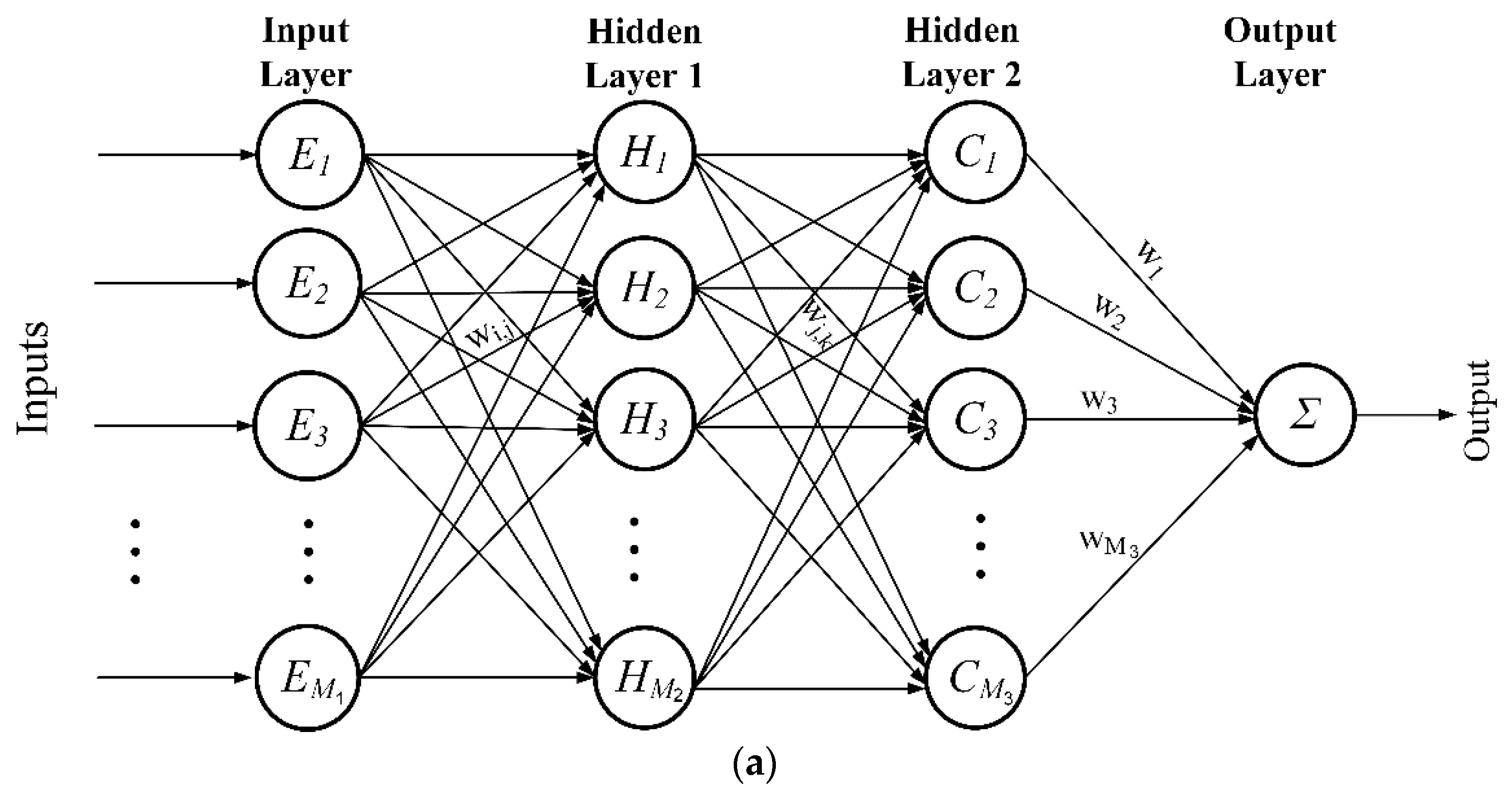
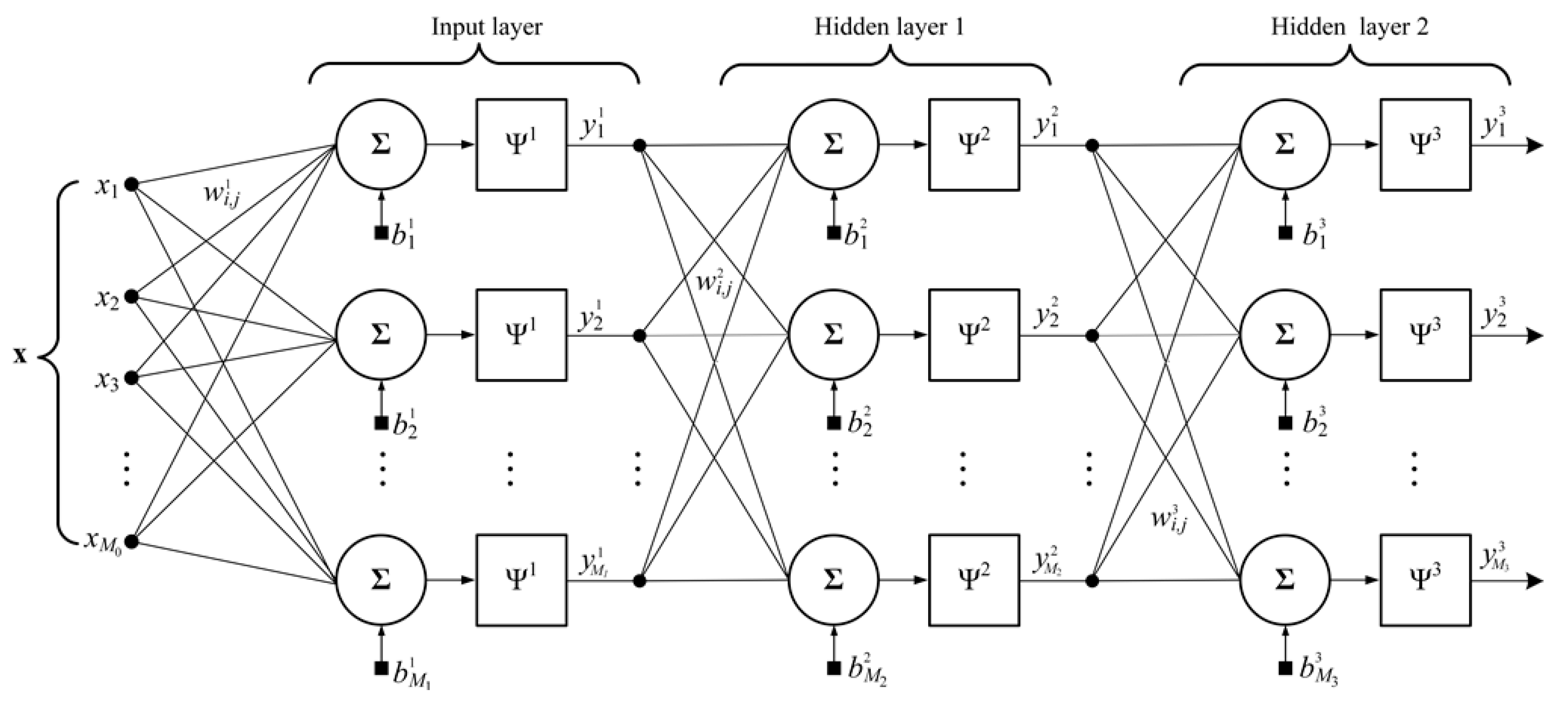
2.1. Artificial Neural Network Architecture

Figure 1 displays a typical architecture of a four-layer MLP ANN. By $M_n$, where $n=1,2,\dots ,N$ is denoted the number of neurons in each layer. The n index indicates the ANN’s layers of which $n=1$ refers to the input (left-most) layer, and $n=N$ refers to the output (last) layer. The input to the ANN’s first layer is denoted by the vector $\mathbf{x}=\left\{x_1,x_2,\dots ,x_{M_0}\right\}$, where $M_0$ corresponds to the inputs’ number. The n-th layer output is denoted by vector ${\mathbf{y}}^n=\left\{y_1^n,y_2^n,\dots ,y_{M_i}^n\right\}$. The MLP ANN shown in Figure 1 is of sequential architecture meaning that the output of any n-th layer is propagated as input to the immediate successive (n + 1)-th layer. Each neuron’s output for either layer emerges from ${\mathbf{y}}^n={\mathsf{\Psi }}^n\left({\mathbf{y}}^{n-1}{\mathbf{w}}^n+{\mathbf{b}}^n\right)$, where ${\mathsf{\Psi }}^n$ is an appropriately selected activation function, ${\mathbf{b}}^n$ is a vector containing the bias weighing of the n-th layer, and ${\mathbf{w}}^n$ is a matrix containing the synaptic weights $w_{i,j}^n$ (with $i=1,2,\dots ,M_{n-1}$, $j=1,2,\dots ,M_n$), that are readily adjustable pending training by a suitable algorithm.

Four different neural network models were designed in order to solve the forward problem of HHV prediction and the quasi-inverse problem of hydrochar content determination. Each ANN model, with 1 output and 2–4 inputs, was trained, validated, and tested using 70–100 full sets of the appropriate collected data. ANN analysis and simulations were performed in the MATLAB environment, using the deep learning toolbox [31]. In all cases, the powerful Levenberg-Marquardt (LM) learning algorithm was selected, and the hyperbolic tangent sigmoid activation function was adapted for the hidden layer neurons. The training procedure continued until either the training mean square error was less than the error goal of 10⁻⁶ (error achievement criterion), or the maximum number of 1000 consecutive times (epochs) was reached (slow convergence criterion), or the validation mean square error was increasing for more than 6 epochs (overfitting avoidance criterion).

2.2. Pre-Processing of Data

In order to address the problem of large value diversity in the data that might introduce instability upon neural networks’ operation during training leading to poor generalization, prior to the latter, a predefined range was asserted to normalize all hydrochar data. This was conducted for all hydrochar variables using Equation (1) that effectively normalized all data within the range (−1, 1):

$${x^{\prime }}_i=\frac{\left(x_b-x_a\right)\left(x_i-x_{min}\right)}{\left(x_{max}-x_{min}\right)}+x_a$$

(1)

where ${x^{\prime }}_i$ denotes the normalized value for sample $x_i$, $x_a=-1$, $x_b=1$, and $x_{min}$ and $x_{max}$ are the minimum and maximum values of $x_i$, respectively.

Following normalization, the overall dataset was broken into fractions of 70%, 15%, and 15% forming three distinct datasets for training, validation, and testing, respectively. The training dataset was employed during the learning process in order to train and fit the parameters of each ANN model. Τhe validation dataset was employed alongside the training dataset during the learning process in order to validate hyperparameters’ adjustments performed by the learning algorithm and prevent data overfitting. The testing dataset was data kept unseen during the training process by the ANN model and it was then used following completion of the former to evaluate the performance of the ANN model and test its quality.

3. Results

In this section, the authors present the statistical analysis and correlation patterns between hydrocarbon properties along with neural networks deployed for that purpose.

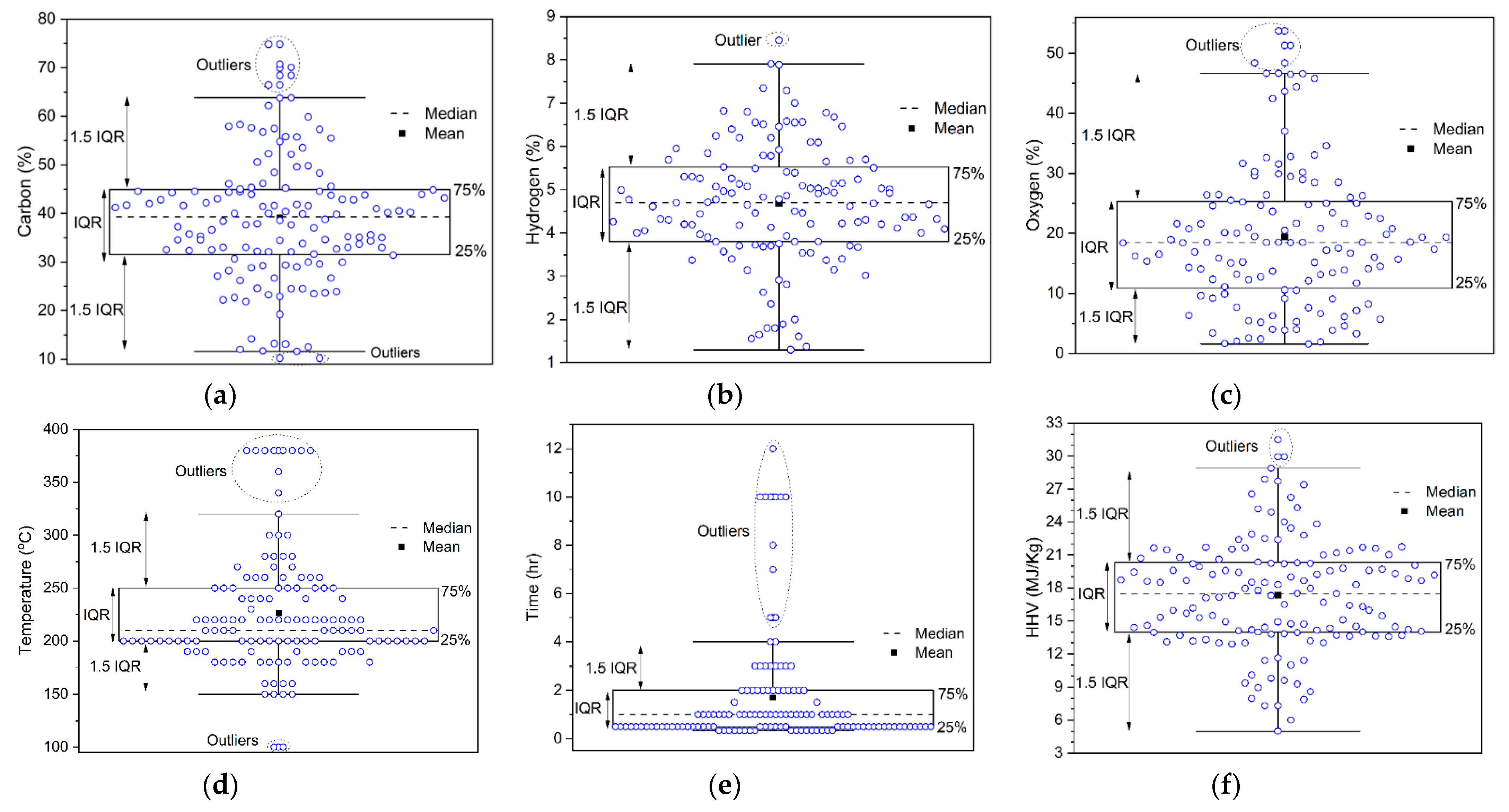
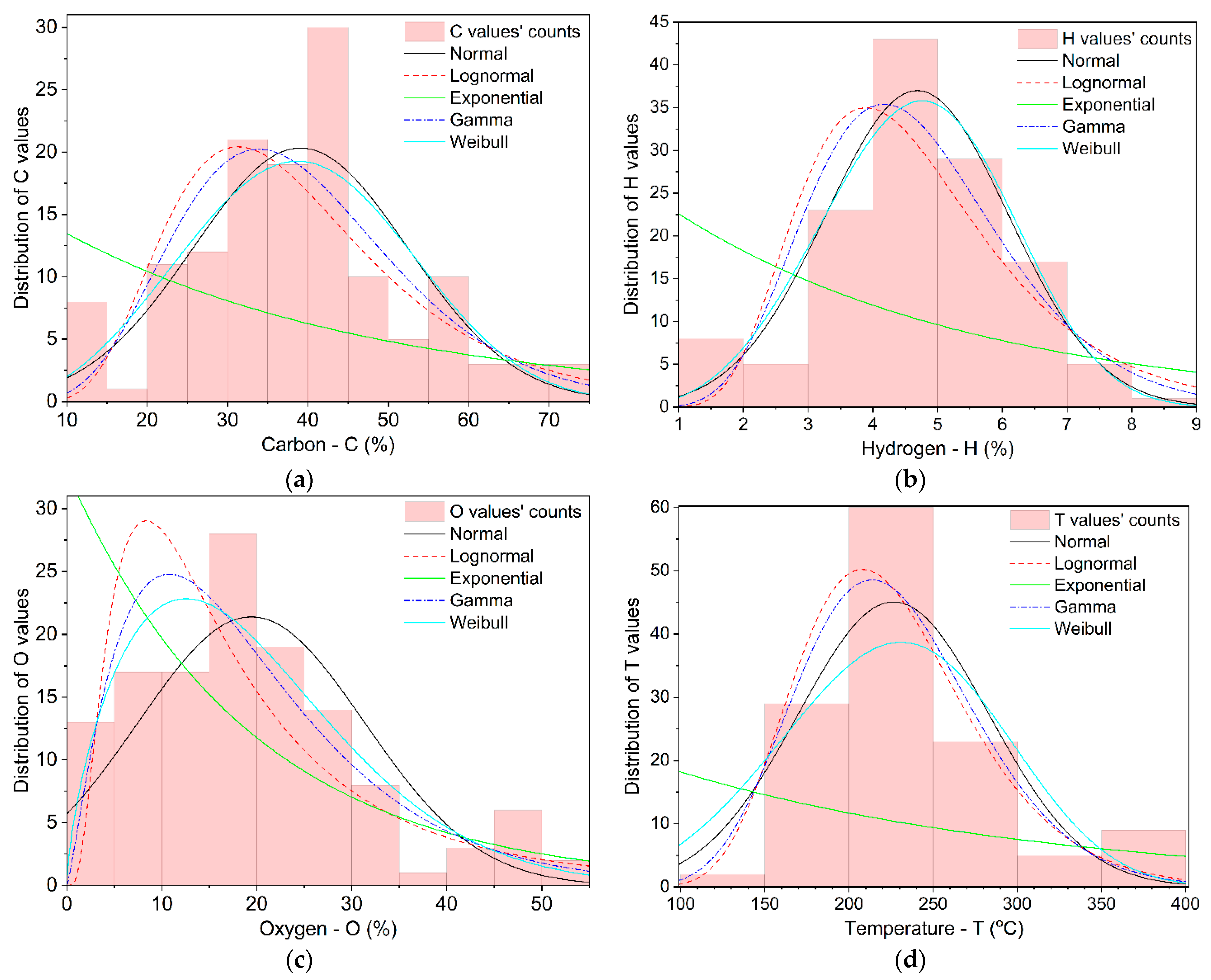
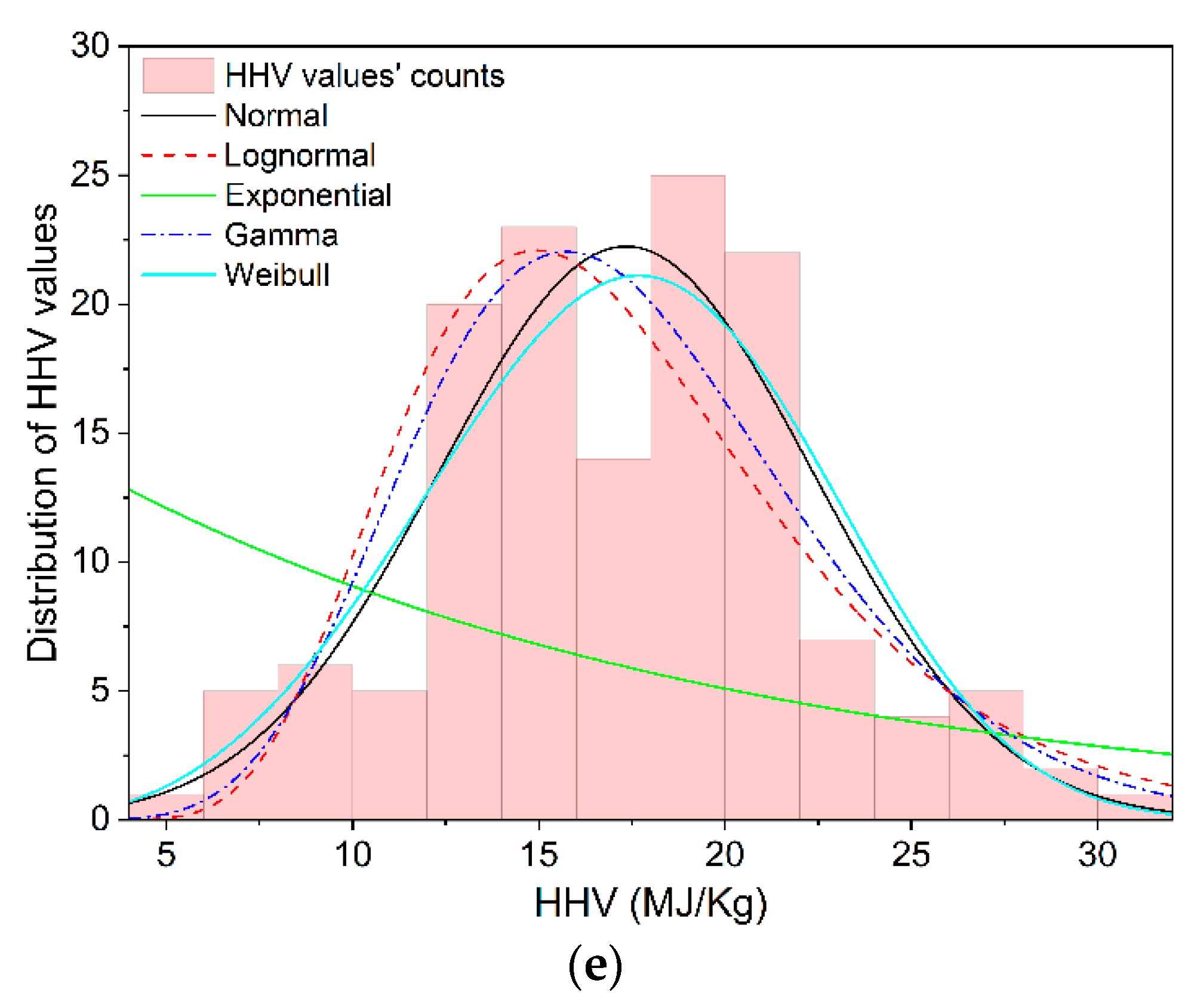
3.1. Hydrochar Properties’ Statistical Analysis

The box and whisker plots in Figure 2 present the statistical distributions of seven hydrochars’ characteristics that were produced during the hydrothermal carbonization of sewage sludge. Data dispersion was examined using the interquartile range (IQR) by dividing datasets into quartiles. On the box and whisker plots from top to bottom, there are five lines that represent the (i) maximum value, (ii) third quartile (Q3), median, first quartile (Q1), and minimum value of the corresponding dataset. The mean value is displayed by the rectangular marker, while the distinct dotted ellipsoids display outliers in the data set, which were excluded from the training process. Useful data of every plot were values ranging in-between Q1 − 1.5IQR and Q3 + 1.5IQR, with IQR = Q3 − Q1, whilst outlier data values were in the range of less than Q1 − 1.5IQR or more than Q3 + 1.5IQR.

Regarding the input parameters, the median, and mean temperatures during the hydrothermal carbonization process were respectively 209.87 and 226.61 °C, and equivalently the median and mean times were 1.01 h and 1.68 h, respectively. The range of values regarding temperatures was from 149.97 to 319.98 °C as shown in Figure 2a, and regarding time was from 0.33 to 4 h as shown in Figure 2b, respectively. The median and mean values of the hydrochars’ content were 39.29% and 39.07% for carbon, 18.49% and 19.49% for oxygen, and 4.69% and 4.68% for hydrogen, with a variance in the range 11.61–63.8%, 1.54–46.68%, and 1.3–7.9%, respectively, as shown in Figure 2c–e. In regard to the output parameters, i.e., the higher heating value and the percentage of solid yield, the median and mean values were 17.48 MJ/Kg and 17.32 MJ/Kg for the former and 64.91% and 66.36% for the latter, with a variance in the range of 5.01–28.90 MJ/Kg and 30.29–96.19%, as shown in Figure 2f,g, respectively.

3.2. Correlation Patterns Between Hydrochar Properties

The Pearson correlation coefficient (PCC), r was deployed to determine the relationship between any pair of the seven overall SSH characteristics, as shown in Equation (2):

$$r_{yz}=\frac{{\displaystyle \sum _{i=1}^N\left(y_i-\overline{y}\right)\hspace{0.17em}{\displaystyle \sum _{i=1}^N\left(z_i-\overline{z}\right)}}}{\sqrt{{\displaystyle \sum _{i=1}^N\left(y_i-\overline{y}\right){\hspace{0.17em}}^2}}\hspace{0.17em}\sqrt{{\displaystyle \sum _{i=1}^N\left(z_i-\overline{z}\right){\hspace{0.17em}}^2}}}$$

(2)

where $y$ and $z$ correspond to two randomly selected variables that are to be examined for linear dependence (i.e., correlation), $\overline{y}$ and $\overline{z}$ correspond to the equivalent means, and $y_i$ and $z_i$ represent the individual values obtained by the variables from the respective datasets.

Τhe seven-by-seven Pearson correlation matrix presented in

Table 1. Hydrochar properties’ Pearson correlation matrix (CI = 95%).

		Temperature	Time	Carbon	Hydrogen	Oxygen	HHV	Solid Yield
Temperature	r	1.000	−0.162	−0.067	−0.229	−0.440	0.055	−0.310
	p-value	--	0.058	0.474	0.015	0.000	0.550	0.003
Time	r	−0.162	1.000	0.092	−0.099	−0.173	−0.111	0.061
	p-value	0.058	--	0.329	0.306	0.076	0.226	0.571
Carbon	r	−0.067	0.092	1.000	0.719	0.202	0.821	−0.246
	p-value	0.474	0.329	--	0.000	0.022	0.000	0.049
Hydrogen	r	−0.229	−0.099	0.719	1.000	0.416	0.694	−0.050
	p-value	0.015	0.306	0.000	--	0.000	0.000	0.705
Oxygen	r	−0.440	−0.173	0.202	0.416	1.000	0.172	0.460
	p-value	0.000	0.076	0.022	0.000	--	0.060	0.000
HHV	r	0.055	−0.111	0.821	0.694	0.172	1.000	−0.398
	p-value	0.550	0.226	0.000	0.000	0.060	--	0.000
Solid Yield	r	−0.310	0.061	−0.246	−0.050	0.460	−0.398	1.000
	p-value	0.003	0.571	0.049	0.705	0.000	0.000	--
Significance Level	p < 0.05	Temperature	Time	Carbon	Hydrogen	Oxygen	HHV	Solid Yield
		H, O, SY	--	H, O, HHV, SY	T, C, O, HHV	T, C, H, SY	C, H, SY	T, C, O, HHV

, reveals either positive or negative correlations in the case where the corresponding significance level p becomes less than 0.05. In effect, higher heating values appear to be positively correlated with the content of carbon and hydrogen, whilst with respect to solid yield, a negative correlation was observed. Likewise, carbon content was observed to be positively correlated with the contents of hydrogen and oxygen content as well as higher heating values, but a negative correlation was once more obtained with respect to solid yield.

The value of r from Equation (2) was used to denote the relation between any two hydrochar properties, where higher PCC values point towards closer relations. As such, HHV appears to be closely related to the content of carbon (r = 0.821) and to a lesser extent to the content of hydrogen (r = 0.693) and that of solid yield (r = −0.398). A minimal correlation was observed regarding temperature (r = 0.054) and time of HTC (r = −0.111). Likewise, carbon content demonstrated a high correlation with HHV, hydrogen and oxygen content, and solid yield, and a low correlation with respect to time and temperature.

For the five hydrochar parameters (carbon, hydrogen, oxygen, temperature, and higher heating value) that exhibit stronger correlations according to Table 1, Figure 3 presents the original and approximating distributions of their values. In each case, the corresponding normal, lognormal, exponential, Gamma, and Weibull distributions are plotted in order to approximate the original data distributions. According to the goodness of fit tests: (a) the normal distribution seems to be suitable for the hydrogen and HHV values, and cannot be rejected for the carbon and oxygen values, (b) the lognormal distribution cannot be rejected for the C and HHV values, but it is rejected for the H and O values, (c) the exponential distribution does not fit any biochar values, (d) the Gamma distribution is appropriate for the O and HHV values, and cannot be rejected for the C and H values, (e) the Weibull distribution is satisfactory for the H, O, and HHV values, and cannot be rejected for the C values, and (f) no distribution is acceptable for the T values.

Neural networks were deployed to investigate the aforementioned relations and determine the influencing factors related to HHV. For that purpose, four distinct artificial neural networks were developed: (i) ${\mathrm{NN}}_1$ aiming to predict HHV values given input factors of carbon, hydrogen, and oxygen, either of close or loose relation; (ii) ${\mathrm{NN}}_2$ aiming to predict HHV values when only the factors of closer relation, the carbon and hydrogen content are given. Quasi-inverse neural networks were developed in the case of (iii) ${\mathrm{NN}}_3$ and (iv) ${\mathrm{NN}}_4$, where the former (iii) aims to predict the carbon content given as inputs the factors of close relation, namely hydrogen and oxygen content as well as HHV; the latter (iv) aims to predict hydrogen content given carbon and oxygen content as well as HHV and temperature as inputs. Although according to Pearson’s correlation solid yield is in close relation to HHV and carbon, the obtained experimental data reported in the literature do not suffice to train the aforementioned neural networks.

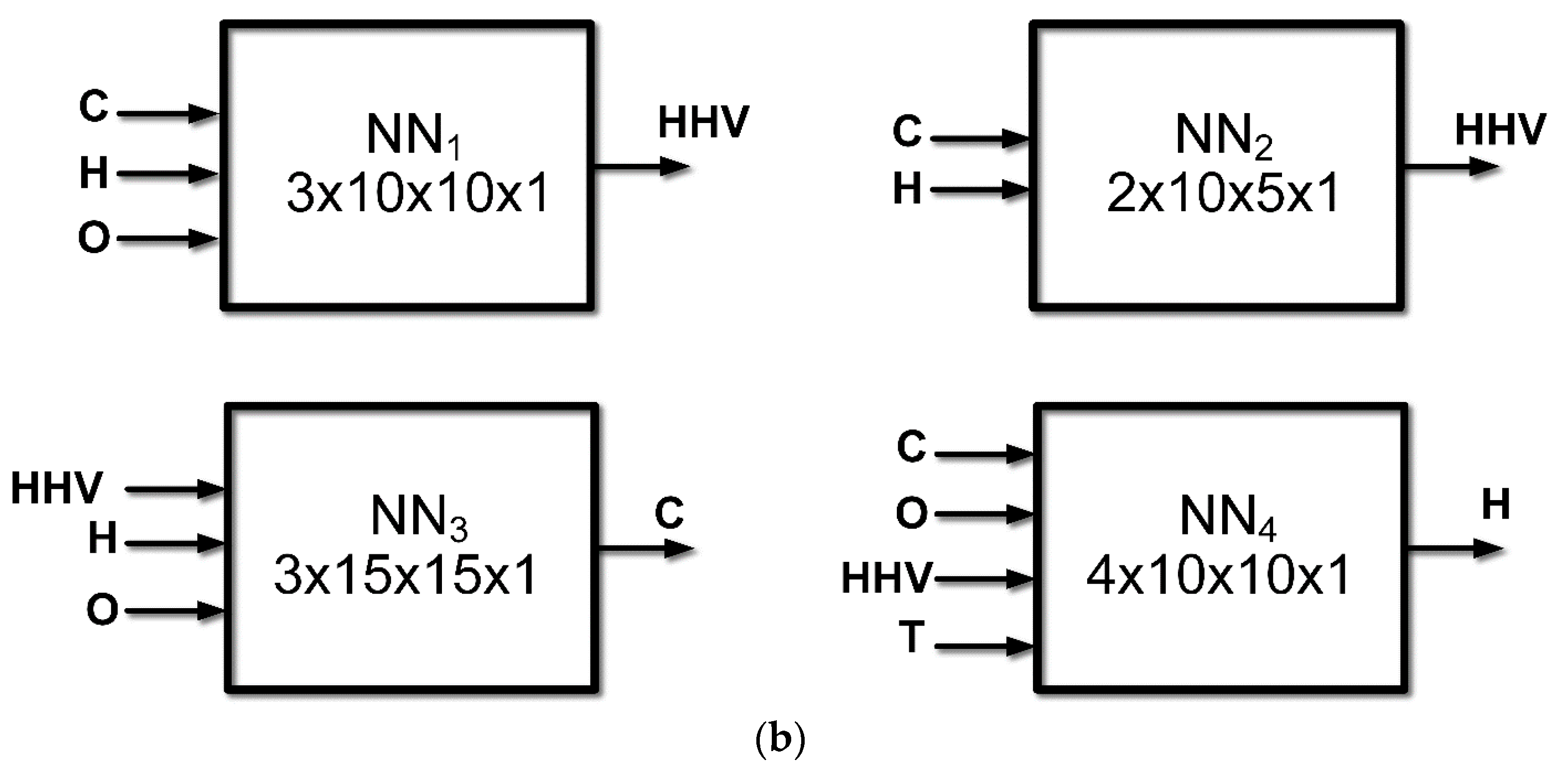
3.3. Artificial Neural Network Modeling

The block diagrams of all four artificial neural network (ANN) models are shown in Figure 4a. The dense, sequential, multilayer perceptron (MLP) architecture was selected for implementation of each of the ANN models in Figure 4b, as it is reported to be a well-established universal approximator [17,18,19,32,33].

Aiming to either solve for the forward problem i.e., that of predicting the hydrochars’ HHV, or to solve for the quasi-inverse problem, i.e., that of determining the required carbon (C) or hydrogen (H) content of hydrochars to obtain specific values for HHV, the architecture of the ANN models displayed in Figure 4b contains a single output and either two, three, or four inputs of various hydrochar parameters. Regarding the forward problem, the ${\mathrm{NN}}_1$ has a single output, i.e., HHV, and three inputs, carbon, hydrogen, and oxygen, whilst ${\mathrm{NN}}_2$ comprises of a single output, i.e., HHV, and two inputs, carbon and hydrogen. Regarding the quasi-inverse problem, the ${\mathrm{NN}}_3$ has a single output, i.e., carbon, and three inputs i.e., hydrogen, oxygen, and HHV, whilst ${\mathrm{NN}}_4$ comprises of a single output, i.e., hydrogen, and four inputs i.e., carbon, oxygen, HHV, and temperature.

The architecture for all ANN models shown in Figure 4b follows the general block diagrams presented in Figure 1 and Figure 4a. The number of neurons per hidden layer was selected following multiple experiments targeted at minimizing the mean square error (MSE), defined as shown in Equation (3):

$$MSE=\frac{1}{K}{\displaystyle \sum _{k=1}^K{(p_k-e_k)}^2}$$

(3)

where $p_k$ and $e_k$ stand for the k-th prediction by the ANN model and experimentally obtained hydrochar parameters’ values, respectively, while K corresponds to the multitude of values used during training. The trial-and-error approach for each of the four ANN models that minimizes the MSE in each case concluded with 10 × 10, 10 × 5, 15 × 15, and 10 × 10 neurons in the first and second hidden layers of ${\mathrm{NN}}_1$, ${\mathrm{NN}}_2$, ${\mathrm{NN}}_3$, and ${\mathrm{NN}}_4$, respectively.

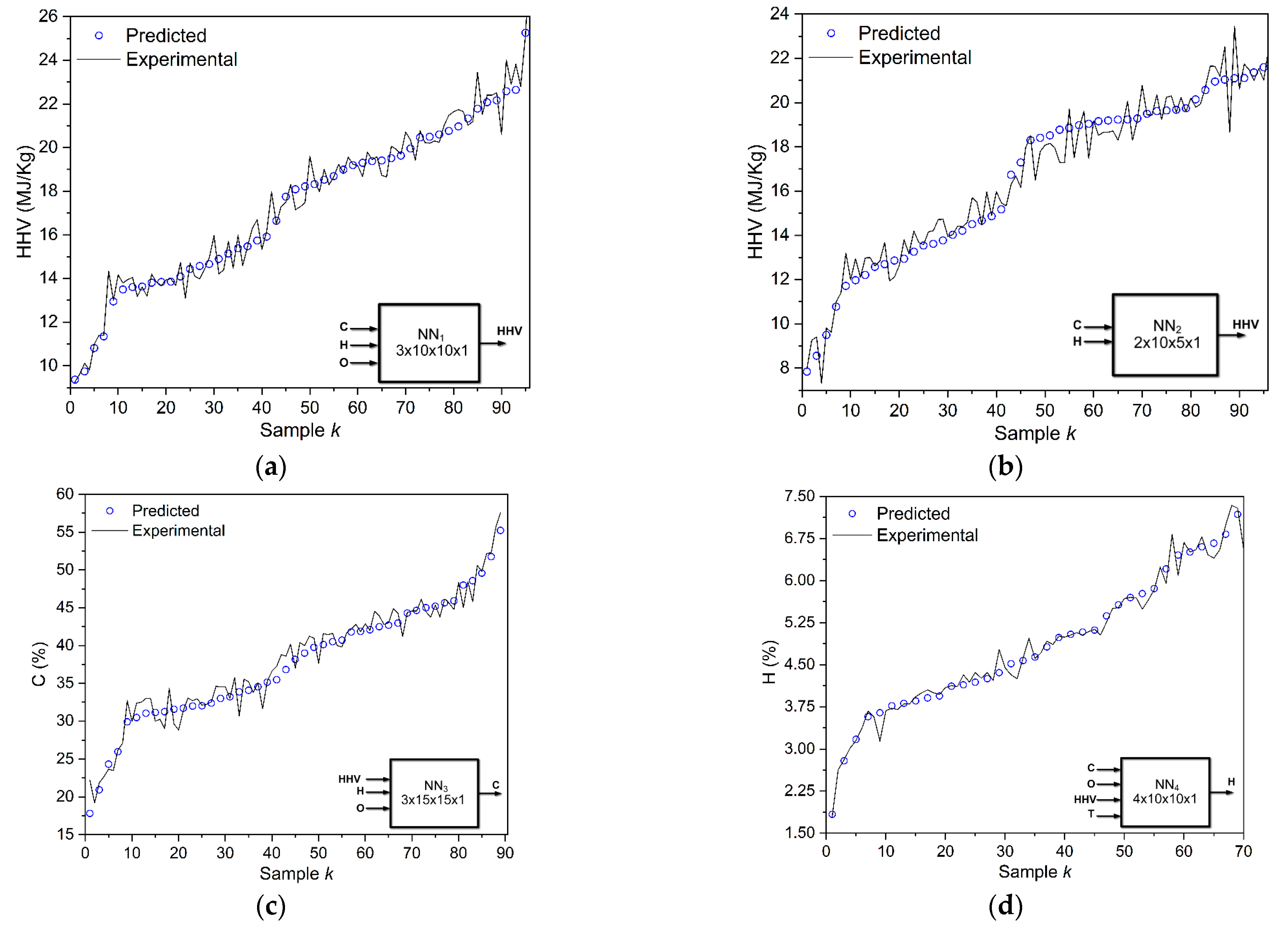
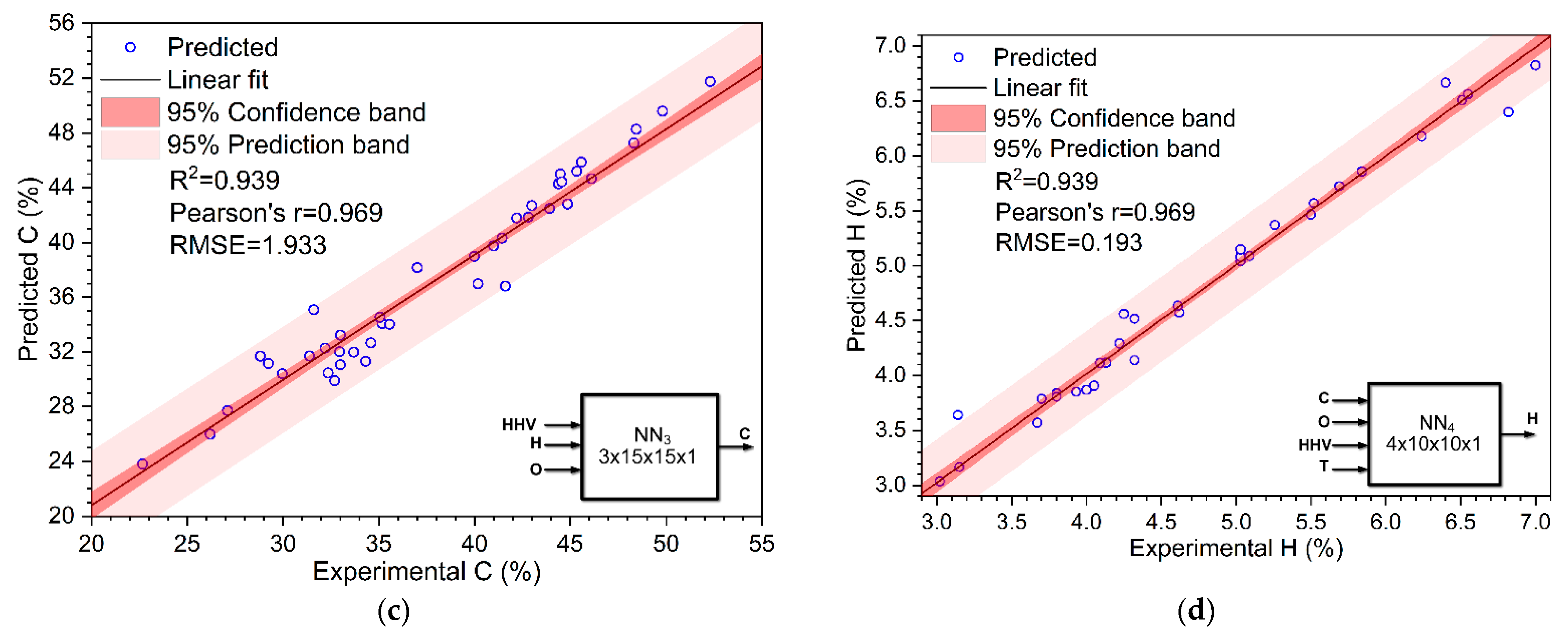
3.4. ANN Models’ Performance

Following completion of the ANNs training and validation processes, the implemented four models were tested with respect to the quality of their performance using the previously unseen testing datasets consisting of quadruples in the form of $\left(C_k^{te},\hspace{0.17em}{O}_k^{te},\hspace{0.17em}{H}_k^{te};\hspace{0.17em}\hspace{0.17em}HH{V}_k^{te}\right)$ regarding ${\mathrm{NN}}_1$, triplets in the form of $\left(C_k^{te},\hspace{0.17em}\hspace{0.17em}{H}_k^{te};\hspace{0.17em}\hspace{0.17em}HH{V}_k^{te}\right)$ regarding ${\mathrm{NN}}_2$, quadruples in the form of $\left(HH{V}_k^{te},\hspace{0.17em}{O}_k^{te},\hspace{0.17em}{H}_k^{te};\hspace{0.17em}\hspace{0.17em}\hspace{0.17em}{C}_k^{te}\right)$ regarding ${\mathrm{NN}}_3$, and quintets in the form of $\left(\hspace{0.17em}{C}_k^{te},\hspace{0.17em}\hspace{0.17em}{O}_k^{te},\hspace{0.17em}\hspace{0.17em}HH{V}_k^{te},\hspace{0.17em}\hspace{0.17em}{T}_k^{te};\hspace{0.17em}\hspace{0.17em}\hspace{0.17em}{H}_k^{te}\right)$ regarding ${\mathrm{NN}}_4$, where $k=1,2,\dots ,K$, and $C_k^{te}$, $O_k^{te}$, $H_k^{te}$, $HH{V}_k^{te}$, and $T_k^{te}$ are the input testing values (or required outputs in the case of the quasi inverse modeling) of the hydrochar carbon, oxygen and hydrogen content, the HHVs, and the HTC temperature, respectively.

Five-fold cross-validation was used to ensure generalization in the operation of the proposed ANNs because of the small amount of data available combined with the requirement for developing unbiased models.

Table 2. Performance metrics following testing of the proposed ANN models using 5-fold cross-validation.

Table 2. Cont.	MAE	RMSE	RE
NN1	0.483	0.622	0.028
NN2	0.189	0.622	0.033
NN3	1.553	2.164	0.041
NN4	0.790	1.035	0.049

outlines the results from the statistical measures calculated herein examining the generalization and prediction capability of the proposed ANNs as well as the evaluation of the models’ performance.

For the sake of completeness, we use and evaluate the most common estimation errors, usually found in the literature [4,17,18,19,29,30,34], which are the root mean squared error (RMSE), the mean absolute error (MAE), the relative error (RE), and the regression coefficient (R²), defined by the following equations:

$$RMSE=\sqrt{\frac{1}{K}{\displaystyle \sum _{k=1}^K{\left(p_k-e_k\right)}^2}}$$

(4)

$$MAE=\frac{1}{{\rm K}}{\displaystyle \sum _{k=1}^K\left|p_k-e_k\right|}$$

(5)

$$RE=\frac{1}{{\rm K}}{\displaystyle \sum _{k=1}^K\frac{\left|p_k-e_k\right|}{e_k}}$$

(6)

$$R^2=1-\frac{{\displaystyle \sum _{k=1}^K{\left(p_k-e_k\right)}^2}}{{\displaystyle \sum _{k=1}^K{\left(e_k-\overline{e}\right)}^2}}$$

(7)

where $p_k$ and $e_k$ are the k-th predicted and experimental values of the output biochar, i.e., $HH{V}_k^{te}$ for models ${\mathrm{NN}}_1$ and ${\mathrm{NN}}_2$, $C_k^{te}$ for model ${\mathrm{NN}}_3$, and $H_k^{te}$ for model ${\mathrm{NN}}_4$, while $\overline{e}$ represents the experimental output values’ average. For example, the MAE measures the error in the same unit with the estimated biochar, while the RE reveals the closeness degree between the measured and the predicted biochar values [34].

Comparisons of the predicted output hydrochar parameters from the ANN models alongside their corresponding measured values of either HHVs, C content, or H content are given in Figure 5. Solid lines correspond to the experimental data reported in the literature, whereas markers indicate the predicted values from the ANNs of either HHV or carbon content as shown in the inset. The predicted outputs of all ANN models were presented with respect to their equivalent experimental values as shown in Figure 6. The R², r, and RMSE values in Figure 6a–d correspond to the full datasets available for ${\mathrm{NN}}_1$–${\mathrm{NN}}_4$, while the performance metrics values in Table 2 refer to the five-fold cross-validation of the proposed ANN models. From the results, it is made apparent that the developed ANN models were capable of predicting both the HHVs and the C content and H content. In comparison, the performance of ${\mathrm{NN}}_1$ and ${\mathrm{NN}}_4$ appears to be slightly better, yet, the overall performance of all ANNs exhibited sufficient accuracy. While the overall performance and R² values obtained by all models were acceptable, ${\mathrm{NN}}_1$ with R² = 0.974 and r = 0.986 appeared to outperform ${\mathrm{NN}}_2$ with R² = 0.936 and r = 0.967. In the case of the quasi-inverse ANNs, ${\mathrm{NN}}_3$ with R² = 0.939 and r = 0.969 appeared to outperform ${\mathrm{NN}}_4$ with R² = 0.747 and r = 0.864.

As is made evident in Figure 5a,b and Figure 6a,b, the AΝΝ models were able to predict the HHVs values of SSHs. The minor limitations in performance are attributed to: (a) the heterogeneous experimental data employed for training, validating, and testing the ANN models, as they were collected from various literature papers related to a wide spectrum of experimental conditions, (b) the unavoidable presence of multivalued data, as various different published works investigating HTC of several sewage sludge materials with discrete biochar characteristics (used as input data C, O, H, T, t) resulted in very similar or even identical HHVs (used as output data HHV), and c) the dimensionality of input variables as model performance is only improved when important input variables are used [35,36].

4. Discussion

ANNs are useful computational tool, highly capable of identifying the intricate relationships between certain input and output data. Compared with the other statistical approaches, ANNs offer a high level of accuracy in forecasting the outcome. In this work, we have applied ANN to predict the HHV of SSHs by using the data collected from published studies. The studies we examined show that the mean HHV of SSHs was 17.32 MJ/kg, which agrees with the previous study that reported that SSHs have a fuel quality similar to lignite (HHV 15–25 MJ/kg) [37]. In the production of hydrochar, the temperature was reported to be the most influential parameter [38]. We have found that the average temperature for the HTC of sewage sludge was 226.61 °C. At the same time, a temperature increase was reported to lead to high ash content, which may adversely affect its fuel properties. As for the elemental composition, the mean carbon, oxygen, and hydrogen content was 39.07%, 19.49% and 4.68%, respectively. According to the Pearson correlation analysis, the HHV closely correlated to carbon (r = 0.821) and hydrogen content (r = 0.693), but negatively correlated with solid yield (r = −0.398). However, the relationship of HHV with temperature and HTC time was weak.

The ANN analysis using the Levenberg-Marquardt (LM) learning algorithm could accurately predict the HVVs of SSHs. Although all four ANNs exhibited sufficient accuracy, NN1 (based on C, H, and O as inputs) performed better at predicting the corresponding output of HHV. In terms of the criteria of R² and RMSE, the proposed ANN models presented quantitative determination of hydrochar properties with high accuracy. Comparing the predicted model performances with the experimental results, NN1, as a forward model, had an R² value of 0.974, and NN3, as an inverse model, had an R² value of 0.939. Given that the chemical composition of sewage sludge greatly differs depending on the treatment process and the source of the sewage, the carbon contents of different hydrochar samples can have significant variation [39]. The implication of the present study is that one can greatly reduce the analysis cost and time to accurately predict HHV of SSHs. Furthermore, in conjunction with the reverse ANN model, one can simply determine the sewage sludge biomass that is the best suitable for producing hydrochar. The correlations between the output (HHV) and input parameters can enable researchers to design and optimize the production method.

The management of sewage sludge has always been problematic for authorities across the world. With the introduction of new regulations, the management strategies shift from storage options to stabilization or valorization [40]. Given that the HTC requires an aqueous medium, sewage sludge is an advantageous biomass due to the elimination of the drying step. HTC of sewage sludge not only reduces the waste volume but also obtains valuable products which may have applications in energy production, wastewater treatment, and soil conditioning. In wastewater treatment, SSHs can be employed as an adsorbent material. Particularly, oxygen-rich functional groups on their surfaces enhance their adsorption selectivity [41]. Still, their limited porosities may require additional physical and chemical activation processes to promote pore development. SSHs can be a good alternative safe fuel with high HHV and ignition temperature. Therefore, the production of biofuel through the HTC of sewage sludge is a cost-effective approach since a moderate temperature of 200 °C and a short holding time (30 min) is enough to achieve a 50% recovery rate [38]. Considering that sewage sludge retains most of the macronutrients, it could be used as an agricultural fertilizer. Moreover, the application of these products in the soil can increase the water retention capacity because of their affinities towards water [42]. However, unlike organic substances, the heavy metals accumulate in the hydrochar without being degraded during the hydrothermal carbonization. Therefore, the risks associated with the release of heavy metals should be carefully assessed before field application. Overall, further studies are needed to improve our knowledge about the mechanisms of the HTC process so that a stronger control can be established over the process parameters and their relationships between the final products. In this regard, the present study can serve as a valuable tool to optimize and control the HTC process of sewage sludge using advanced computational approaches such as ANN-based modeling.

5. Conclusions

On a worldwide level, sewage sludge remains a waste material with limited exploitation pathways. The conversion of sewage sludge to hydrochar through hydrothermal carbonization appears to be a feasible alternative for the production of a novel material with tunable properties, with a high enough HHV to be used as a biofuel. However, the composition of sewage sludge varies considerably, therefore, HTC cannot be easily standardized to produce hydrochars with high HHVs. Towards this purpose, ANNs were successfully applied and correlated the HHVs to the C, H, and O contents. Overall, this modeling approach will assist in the development of engineered hydrochars and allow researchers to fine-tune the HTC conditions to produce hydrochars of a minimum biofuel quality.

References

1. Libra, J.A.; Ro, K.S.; Kammann, C.; Funke, A.; Berge, N.D.; Neubauer, Y.; Titirici, M.-M.; Fühner, C.; Bens, O.; Kern, J.; et al. Hydrothermal carbonization of biomass residuals: A comparative review of the chemistry, processes and applications of wet and dry pyrolysis. Biofuels 2011, 2, 71–106. [Google Scholar] [CrossRef] [Green Version]
2. Heidari, M.; Dutta, A.; Acharya, B.; Mahmud, S. A review of the current knowledge and challenges of hydrothermal carbonization for biomass conversion. J. Energy Inst. 2019, 92, 1779–1799. [Google Scholar] [CrossRef]
3. Wang, T.; Zhai, Y.; Zhu, Y.; Li, C.; Zeng, G. A review of the hydrothermal carbonization of biomass waste for hydrochar formation: Process conditions, fundamentals, and physicochemical properties. Renew. Sustain. Energy Rev. 2018, 90, 223–247. [Google Scholar] [CrossRef]
4. Vardiambasis, I.O.; Kapetanakis, T.N.; Nikolopoulos, C.D.; Trang, T.K.; Tsubota, T.; Keyikoglu, R.; Khataee, A.; Kalderis, D. Hydrochars as emerging biofuels: Recent advances and application of artificial neural networks for the prediction of heating values. Energies 2020, 13, 4572. [Google Scholar] [CrossRef]
5. Li, S.; Zeng, W.; Jia, Z.; Wu, G.; Xu, H.; Peng, Y. Phosphorus species transformation and recovery without apatitein FeCl3-assisted sewage sludge hydrothermal treatment. Chem. Eng. J. 2020, 399, 125735. [Google Scholar] [CrossRef]
6. Waldmüller, W.; Herdzik, S.; Gaderer, M. Combined filtration and oxalic acid leaching for recovering phosphorus from hydrothermally carbonized sewage sludge. J. Environ. Chem. Eng. 2021, 9, 104800. [Google Scholar] [CrossRef]
7. Medina-Martos, E.; Istrate, I.-R.; Villamil, J.A.; Gálvez-Martos, J.-L.; Dufour, J.; Mohedano, A.F. Techno-economic and life cycle assessment of an integrated hydrothermal carbonization system for sewage sludge. J. Clean. Prod. 2020, 277, 122930. [Google Scholar] [CrossRef]
8. Zhang, C.; Ma, X.; Zheng, C.; Huang, T.; Lu, X.; Tian, Y. Co-hydrothermal Carbonization of Water Hyacinth and Sewage Sludge: Effects of Aqueous Phase Recirculation on the Characteristics of Hydrochar. Energy Fuels 2020, 34, 14147–14158. [Google Scholar] [CrossRef]
9. Lu, X.; Ma, X.; Chen, X. Co-hydrothermal carbonization of sewage sludge and lignocellulosic biomass: Fuel properties and heavy metal transformation behaviour of hydrochars. Energy 2021, 221, 119896. [Google Scholar] [CrossRef]
10. McGaughy, K.; Toufiq Reza, M. Hydrothermal carbonization of food waste: Simplified process simulation model based on experimental results. Biomass Convers. Biorefin. 2018, 8, 283–292. [Google Scholar] [CrossRef]
11. Gallifuoco, A. A new approach to kinetic modeling of biomass hydrothermal carbonization. ACS Sustain. Chem. Eng. 2019, 7, 13073–13080. [Google Scholar] [CrossRef]
12. Conag, A.T.; Villahermosa, J.E.R.; Cabatingan, L.K.; Go, A.W. Predictive HHV model for raw and torrefied sugarcane residues. Waste Biomass Valorization 2019, 10, 1929–1943. [Google Scholar] [CrossRef]
13. Vallejo, F.; Díaz-Robles, L.A.; Vega, R.; Cubillos, F. A novel approach for prediction of mass yield and higher calorific value of hydrothermal carbonization by a robust multilinear model and regression trees. J. Energy Inst. 2020, 93, 1755–1762. [Google Scholar] [CrossRef]
14. Akdeniz, F.; Biçil, M.; Karadede, Y.; Özbek, F.E.; Özdemir, G. Application of real valued genetic algorithm on prediction of higher heating values of various lignocellulosic materials using lignin and extractive contents. Energy 2018, 160, 1047–1054. [Google Scholar] [CrossRef]
15. Tasca, A.L.; Puccini, M.; Gori, R.; Corsi, I.; Galletti, A.M.R.; Vitolo, S. Hydrothermal carbonization of sewage sludge: A critical analysis of process severity, hydrochar properties and environmental implications. Waste Manag. 2019, 93, 1–13. [Google Scholar] [CrossRef] [PubMed]
16. Liodakis, G.; Arvanitis, D.; Vardiambasis, I.O. Neural network based digital receiver for radio communications. WSEAS Trans. Syst. 2004, 3, 3308–3313. [Google Scholar]
17. Kapetanakis, T.N.; Vardiambasis, I.O.; Ioannidou, M.P.; Konstantaras, A.I. Recent Trends on Electromagnetic Environmental Effects for Aeronautics and Space Applications; Nikolopoulos, C.D., Ed.; IGI Global: Hershey PA, USA, 2021; Chapter 7; pp. 186–225. [Google Scholar]
18. Kapetanakis, T.N.; Vardiambasis, I.O.; Ioannidou, M.P.; Maras, A. Neural network modeling for the solution of the inverse loop antenna radiation problem. IEEE Trans. Antennas Propag. 2018, 66, 6283–6290. [Google Scholar] [CrossRef]
19. Kapetanakis, T.N.; Vardiambasis, I.O.; Lourakis, E.I.; Maras, A. Applying neuro-fuzzy soft computing techniques to the circular loop antenna radiation problem. IEEE Antennas Wirel. Propag. Lett. 2018, 17, 1673–1676. [Google Scholar] [CrossRef]
20. Vardiambasis, I.O.; Tsalamengas, J.L.; Fikioris, J.G. Hybrid wave propagation in circularly shielded microslot lines. IEEE Trans. Microw. Theory Technol. 1995, 43, 1960–1966. [Google Scholar] [CrossRef]
21. Vardiambasis, I.O.; Tsalamengas, J.L.; Fikioris, J.G. Plane wave scattering by slots on a ground plane loaded with semicircular dielectric cylinders in case of oblique incidence and arbitrary polarization. IEEE Trans. Antennas Propag. 1998, 46, 1571–1579. [Google Scholar] [CrossRef]
22. Adamidis, G.A.; Vardiambasis, I.O.; Ioannidou, M.P.; Kapetanakis, T.N. Design and implementation of single-layer 4× 4 and 8× 8 Butler matrices for multibeam antenna arrays. Int. J. Antennas Propag. 2019, 1645281, 1–12. [Google Scholar] [CrossRef]
23. Sergaki, E.; Spiliotis, G.; Vardiambasis, I.O.; Kapetanakis, T.; Krasoudakis, A.; Giakos, G.C.; Zervakis, M.; Polydorou, A. Application of ANN and ANFIS for detection of brain tumors in MRIs by using DWT and GLCM texture analysis. Int. Conf. Imaging Syst. Technol. 2018, 1–6. [Google Scholar] [CrossRef]
24. Bhange, V.P.; Bhivgade, U.V.; Vaidya, A.N. Artificial neural network modeling in pretreatment of garden biomass for lignocellulose degradation. Waste Biomass Valorization 2019, 10, 1571–1583. [Google Scholar] [CrossRef]
25. Baruah, D.; Baruah, D.C.; Hazarika, M.K. Artificial neural network based modeling of biomass gasification in fixed bed downdraft gasifiers. Biomass Bioenergy 2017, 98, 264–271. [Google Scholar] [CrossRef]
26. Nasrudin, N.A.; Jewaratnam, J.; Hossain, M.A.; Ganeson, P.B. Performance comparison of feedforward neural network training algorithms in modelling microwave pyrolysis of oil palm fibre for hydrogen and biochar production. Asia Pac. J. Chem. Eng. 2020, 15. [Google Scholar] [CrossRef]
27. Hawthorne, S.B.; Lagadec, A.J.M.; Kalderis, D.; Lilke, A.V.; Miller, D.J. Pilot-scale destruction of TNT, RDX, and HMX on contaminated soils using subcritical water. Environ. Sci. Technol. 2000, 34, 3224–3228. [Google Scholar] [CrossRef]
28. Daskalaki, V.M.; Timotheatou, E.S.; Katsaounis, A.; Kalderis, D. Degradation of Reactive Red 120 using hydrogen peroxide in subcritical water. Desalination 2011, 274, 200–205. [Google Scholar] [CrossRef]
29. Zhu, X.; Wang, X.; Ok, Y.S. The application of machine learning methods for prediction of metal sorption onto biochars. J. Hazard. Mater. 2019, 378, 120727. [Google Scholar] [CrossRef]
30. Li, J.; Pan, L.; Suvarna, M.; Tong, Y.W.; Wang, X. Fuel properties of hydrochar and pyrochar: Prediction and exploration with machine learning. Appl. Energy 2020, 269, 115166. [Google Scholar] [CrossRef]
31. Deep Learning Toolbox v12.1 (2019a); MathWorks, The Inc.: Natick, MA, USA, 1999.
32. Mazumder, S.; Saha, P.; Reza, M.T. Co-hydrothermal carbonization of coal waste and food waste: Fuel characteristics. Biomass Convers. Biorefin. 2020. [Google Scholar] [CrossRef]
33. Mazumder, S.; Saha, P.; McGaughy, K.; Saba, A.; Reza, M.T. Technoeconomic analysis of co-hydrothermal carbonization of coal waste and food waste. Biomass Convers. Biorefin. 2020. [Google Scholar] [CrossRef]
34. Nhuchhen, D.R.; Afzal, M.T. HHV predicting correlations for torrefied biomass using proximate and ultimate analyses. Bioengineering 2017, 4, 7. [Google Scholar] [CrossRef] [Green Version]
35. Verleysen, Μ.; François, D.; Simon, G.; Wertz, V. On the effects of dimensionality on data analysis with neural networks. In Proceedings of the 7th International Work-Conference on Artificial & Natural Neural Networks (IWANN 2003), Menorca, Spain, 3–6 June 2003; Springer: Berlin/Heidelberg, Germany, 2003; Volume 2687, pp. 105–112. [Google Scholar]
36. Konstantaras, A. Deep learning and parallel processing spatio-temporal clustering unveil new Ionian distinct seismic zone. Informatics 2020, 7, 39. [Google Scholar] [CrossRef]
37. Zheng, X.; Jiang, Z.; Ying, Z.; Song, J.; Chen, W.; Wang, B. Role of feedstock properties and hydrothermal carbonization conditions on fuel properties of sewage sludge-derived hydrochar using multiple linear regression technique. Fuel 2020, 271, 117609. [Google Scholar] [CrossRef]
38. Zhao, P.; Shen, Y.; Ge, S.; Yoshikawa, K. Energy recycling from sewage sludge by producing solid biofuel with hydrothermal carbonization. Energy Convers. Manag. 2014, 78, 815–821. [Google Scholar] [CrossRef] [Green Version]
39. Wang, L.; Chang, Y.; Li, A. Hydrothermal carbonization for energy-efficient processing of sewage sludge: A review. Renew. Sustain. Energy Rev. 2019, 108, 423–440. [Google Scholar] [CrossRef]
40. Teoh, S.K.; Li, L.Y. Feasibility of alternative sewage sludge treatment meth-ods from a lifecycle assessment (LCA) perspective. J. Clean. Prod. 2020, 247, 119495. [Google Scholar] [CrossRef]
41. Han, L.; Ro, K.S.; Sun, K.; Sun, H.; Wang, Z.; Libra, J.A.; Xing, B. New evidence for high sorption capacity of hydrochar for hydrophobic organic pollutants. Environ. Sci. Technol. 2016, 50, 13274–13282. [Google Scholar] [CrossRef] [PubMed]
42. Tasca, A.L.; Stefanelli, E.; Galletti, A.M.R.; Gori, R.; Mannarino, G.; Vitolo, S.; Puccini, M. Hydrothermal carbonization of sewage sludge: Analysis of process severity and solid content. Chem. Eng. Technol. 2020, 43, 2382–2392. [Google Scholar] [CrossRef]
Figure 1. Typical architecture of a one input, two hidden, and one output layered feed-forward MLP ANN.
Energies 14 03000 g001
Figure 2. Box and whisker plots of the values related to SSHs’ composition variables (carbon (a), hydrogen (b), oxygen (c), temperature (d), time (e), and HHV (f)). The data of each dataset are represented as blue markers and divided into quartiles. Each plot depicts the minimum value, the first quartile (Q1), the median, the third quartile (Q3), and the maximum value of the dataset (as five bottom to top horizontal lines), and the mean value (as a rectangular marker). The data within the range from Q1 − 1.5IQR to Q3 + 1.5IQR (where IQR = Q3 − Q1) are considered useful, while the data outside this range are rejected as outliers (enclosed inside dotted ellipsoids).
Energies 14 03000 g002
Figure 3. Plots of the distributions of the C (a), H (b), O (c), T (d), and HHV (e) values. The original data (bar diagrams) and the corresponding normal (black solid line), lognormal (red dashed line), exponential (green solid line), Gamma (blue dash-dotted line), and Weibull (light blue solid line) approximating distributions of their values are depicted in each case.
Energies 14 03000 g003aEnergies 14 03000 g003b
Figure 4. Layout of neural network models for hydrothermal carbonization. (a) M 1 , M 2 , M 3 , and M 4 indicate the numbers of neurons in the input, hidden, and output layers. (b) For either NN 1 4 , input hydrochar parameters appear on the left, the crisp output parameter appears on the right, and the in-box information corresponds to the values of M 1 , M 2 , M 3 , and M 4 .
Energies 14 03000 g004aEnergies 14 03000 g004b
Figure 5. Experimental H H V k t e (a,b), C k t e (c), H k t e (d) versus predicted H H V k p r (a,b), C k p r (c), H k p r (d) output biochar values.
Energies 14 03000 g005
Figure 6. Predicted and experimental data regression analysis for: (a) HHV using NN 1 ; (b) HHV using NN 2 ; (c) carbon using NN 3 ; (d) hydrogen using NN 4 .
Energies 14 03000 g006aEnergies 14 03000 g006b