
Computing Localized Breakthrough Curves and Velocities of Saline Tracer from Ground Penetrating Radar Monitoring Experiments in Fractured Rock

 , , , , and
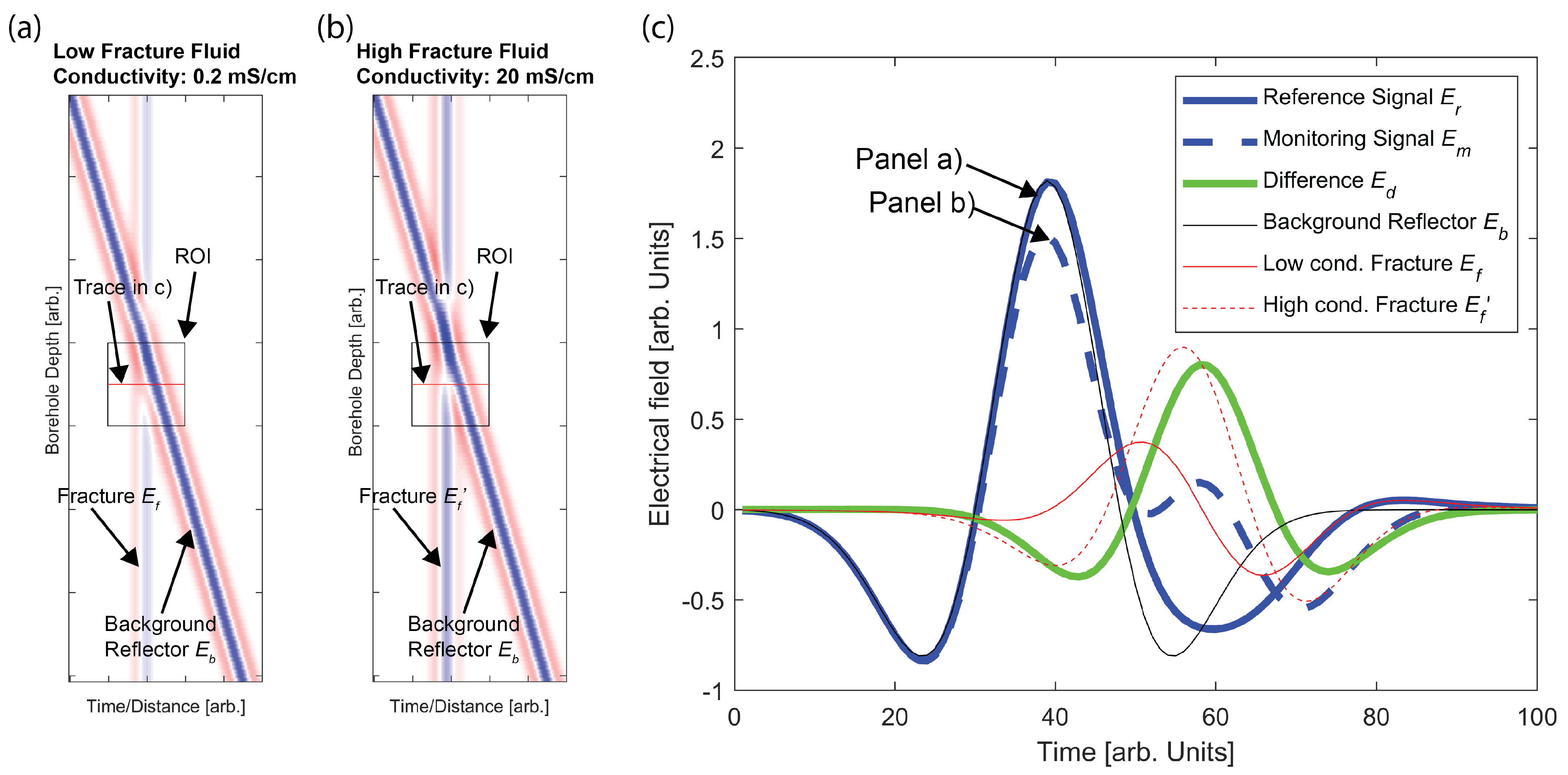
Abstract
1. Introduction
2. Methods
2.1. Breakthrough Curves from Difference Reflection Imaging
2.1.1. Benefits of Difference Reflection Imaging
2.1.2. Difference Radar Breakthrough Curves
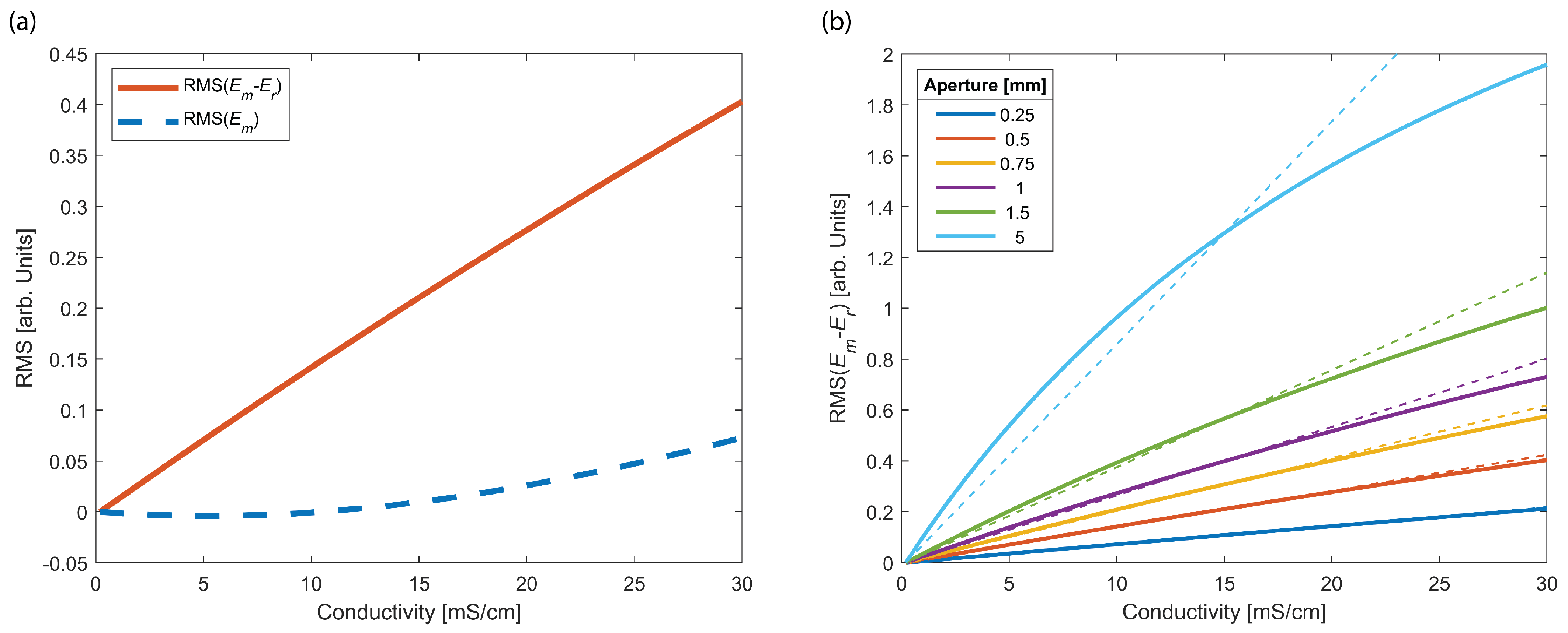
2.1.3. Limitations
2.2. Average Flow Path Velocity Distribution
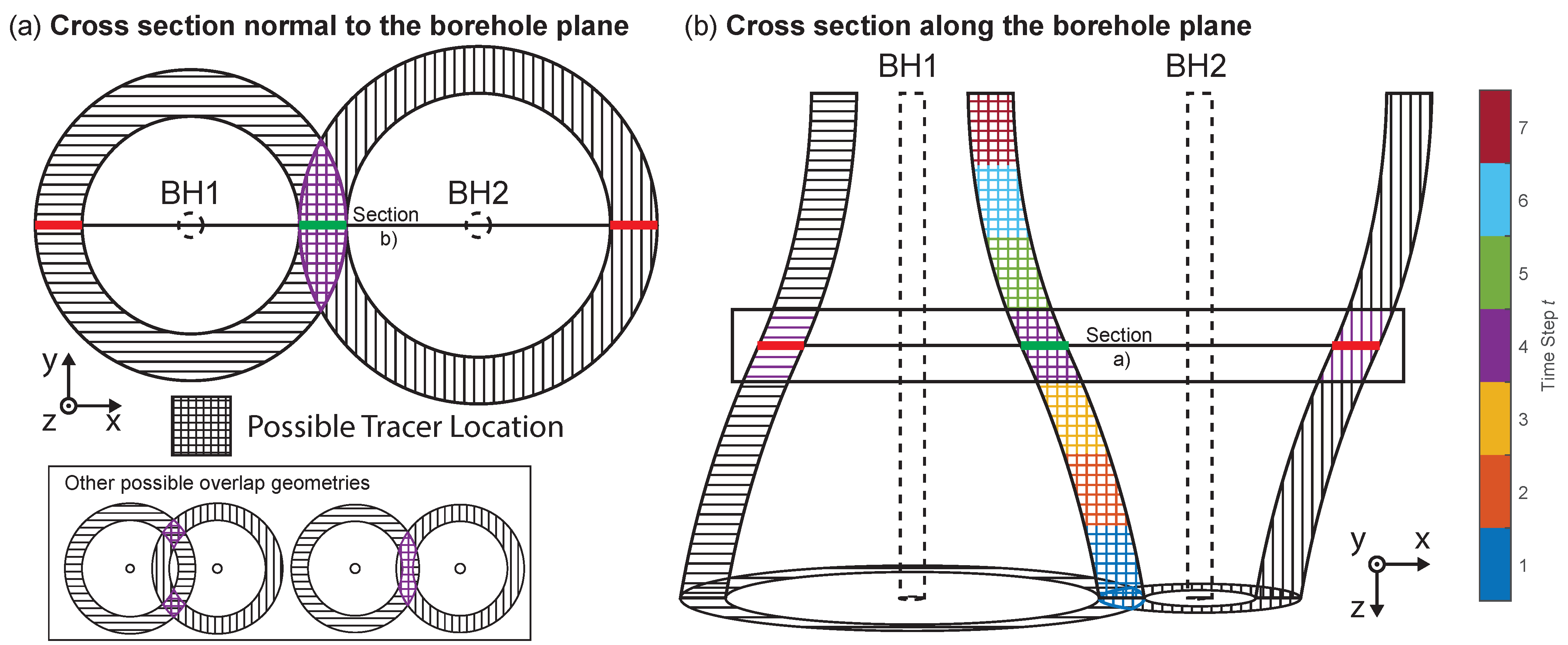
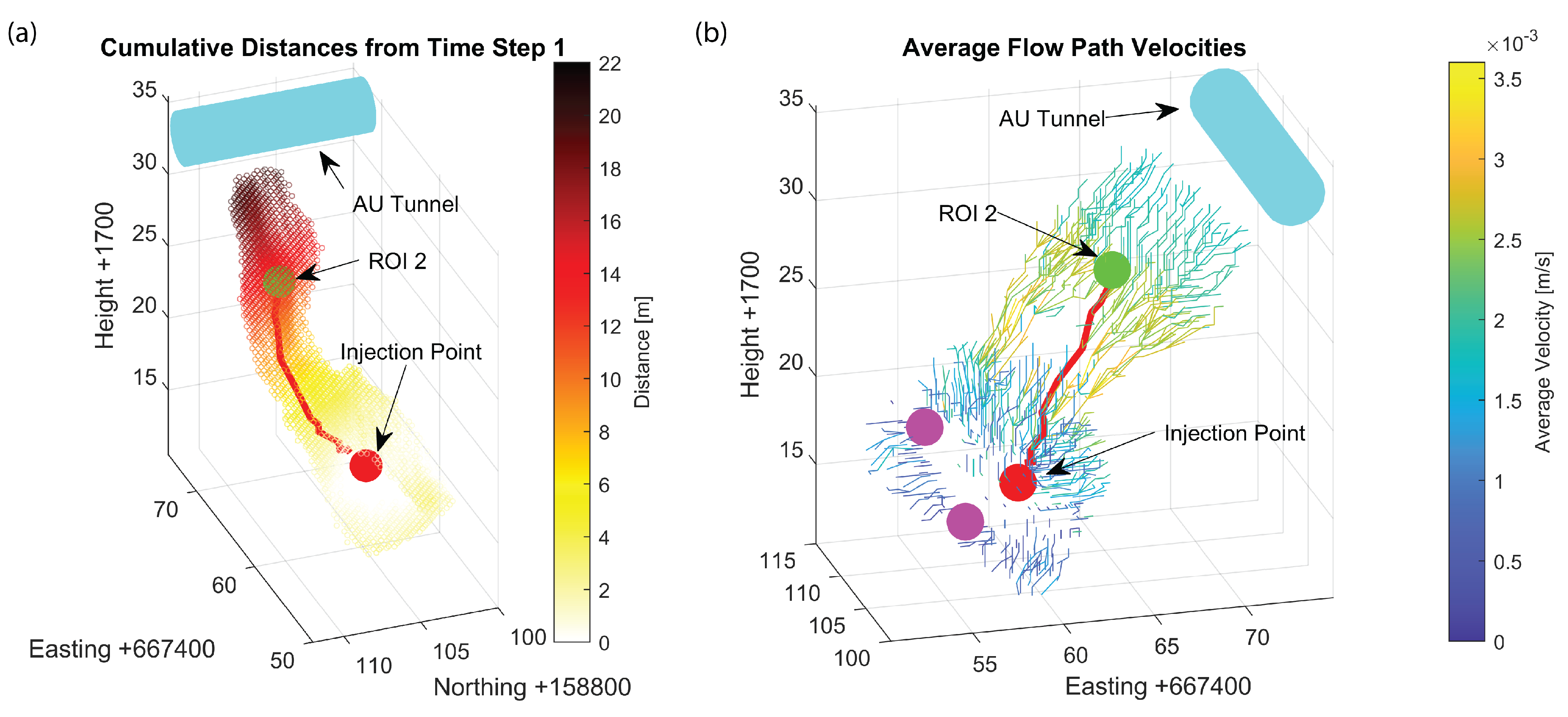
2.2.1. Flow Path Reconstruction
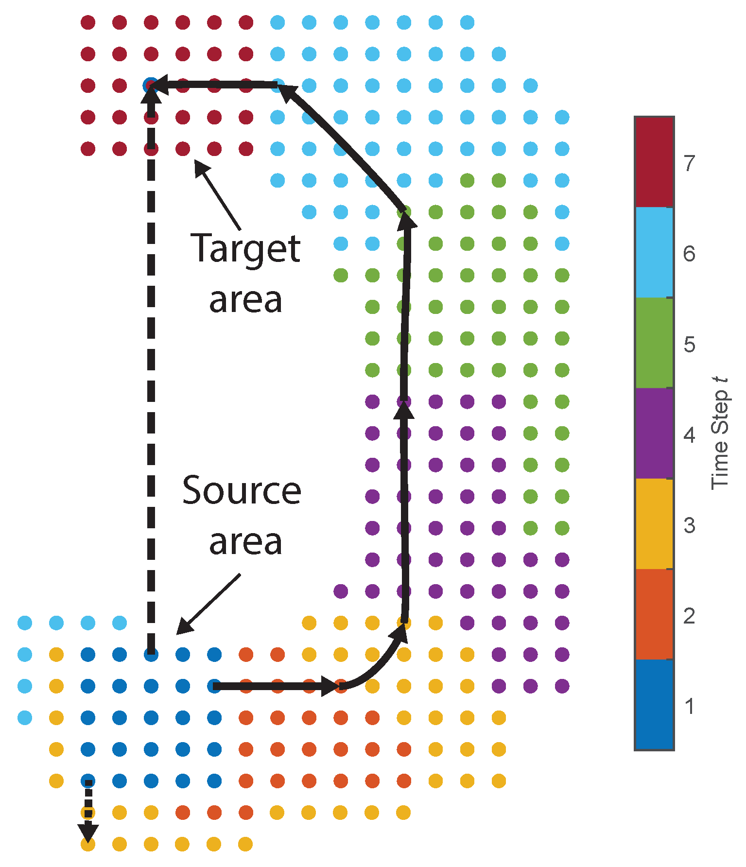
2.2.2. Average Flow Path Velocity Calculation
2.2.3. Limitations
3. Application to Field Data Set
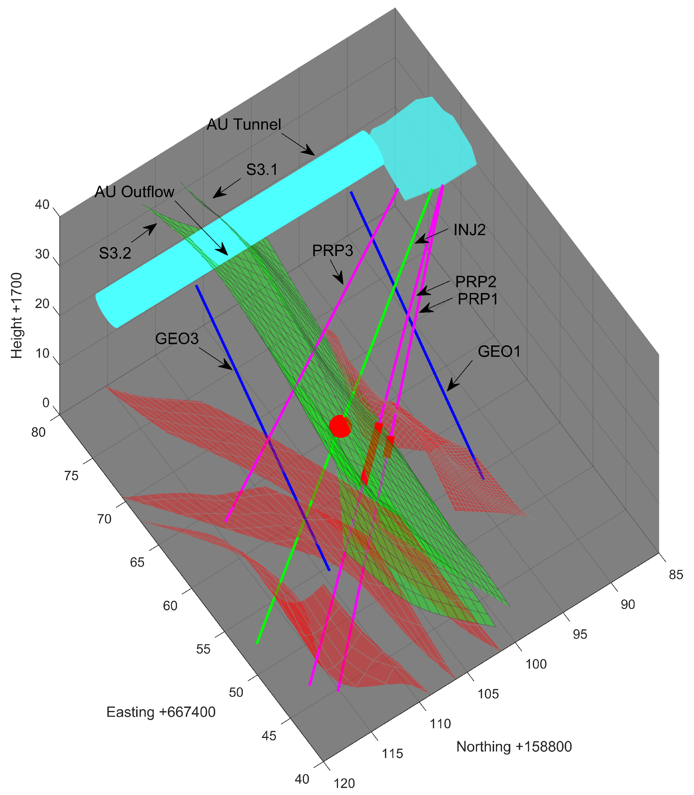
3.1. ISC Experiment at the Grimsel Test Site
3.2. Tracer Experiments
3.3. GPR Data Acquisition and Processing
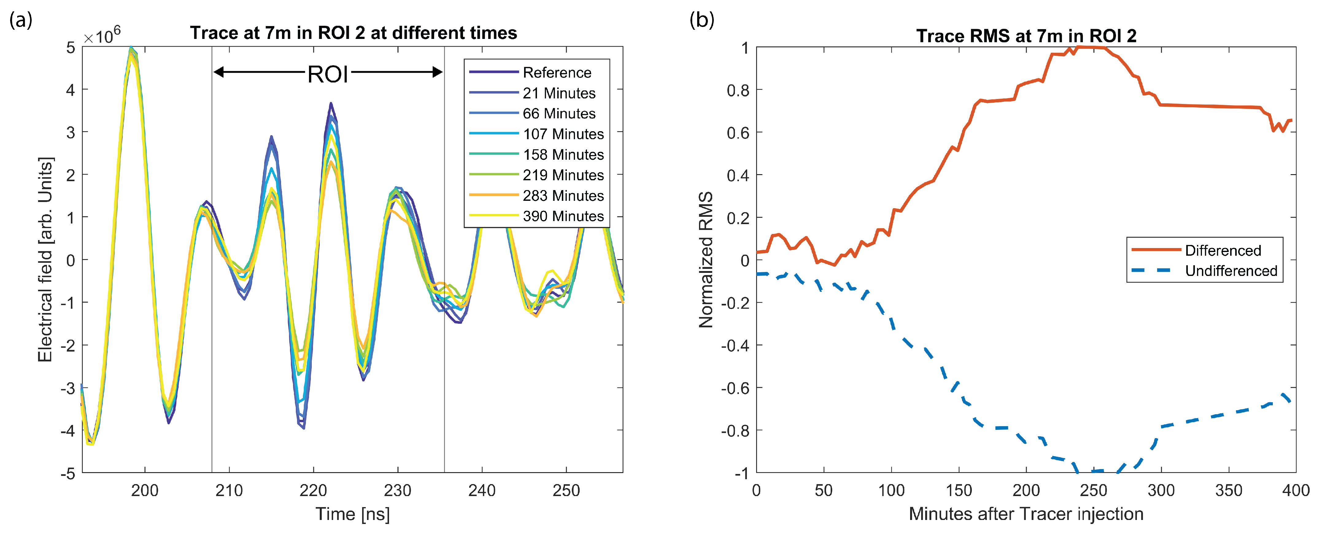
3.4. Breakthrough Curves from Difference Reflection Imaging
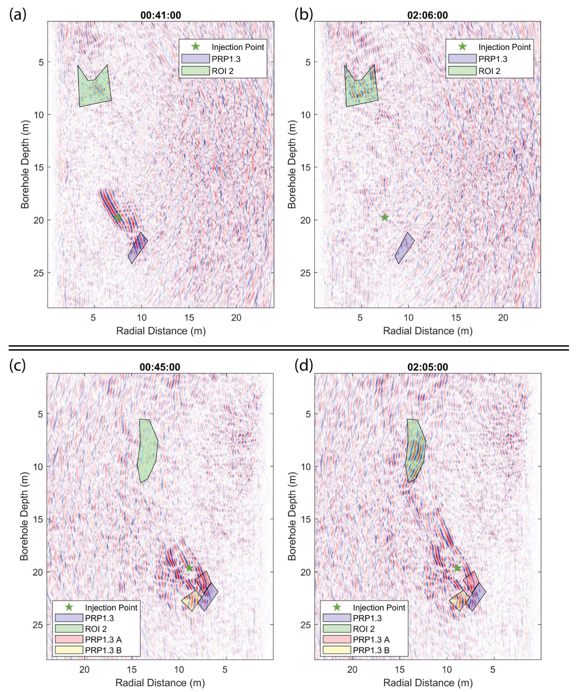
3.4.1. ROI Selection
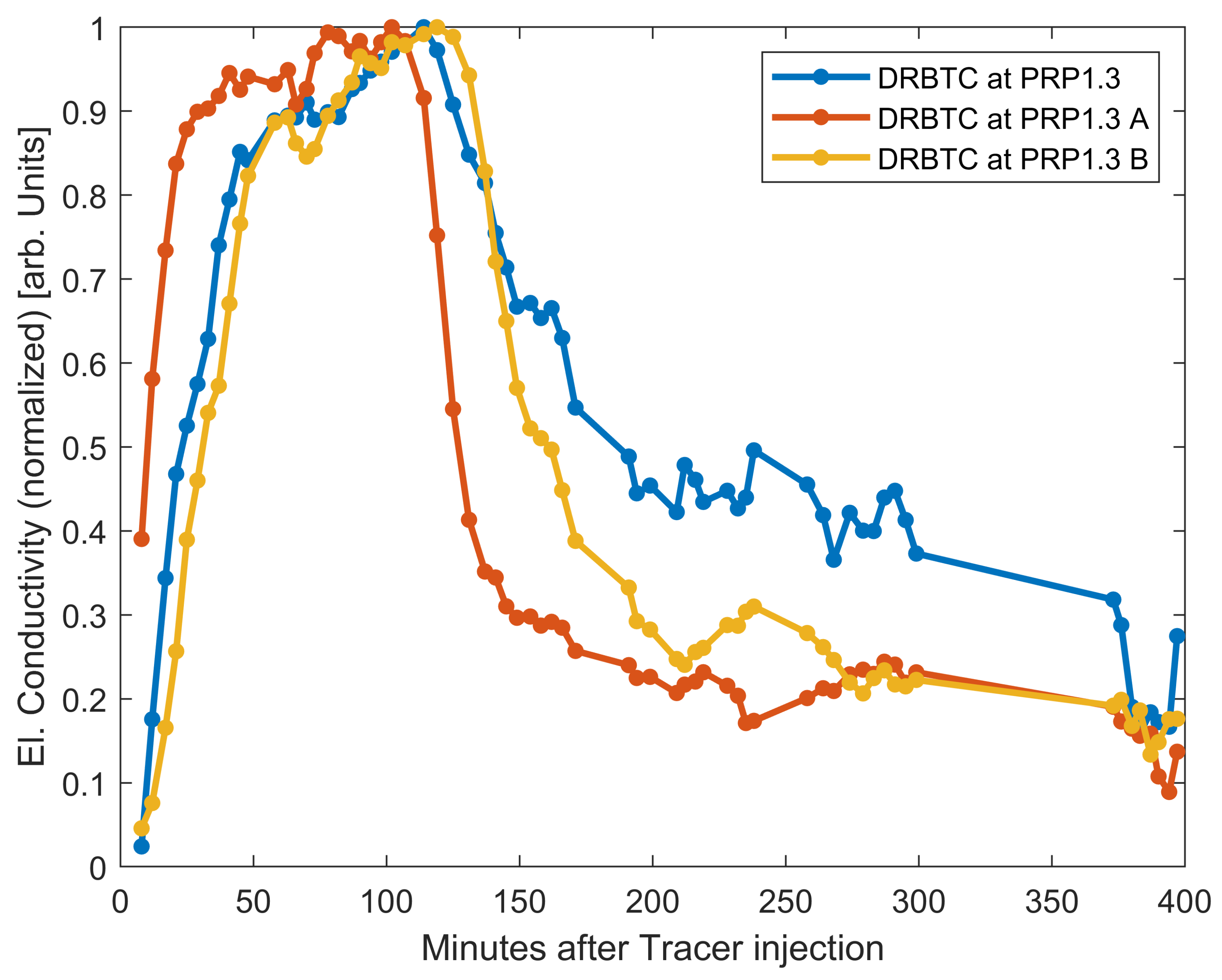
3.4.2. DRBTC Results
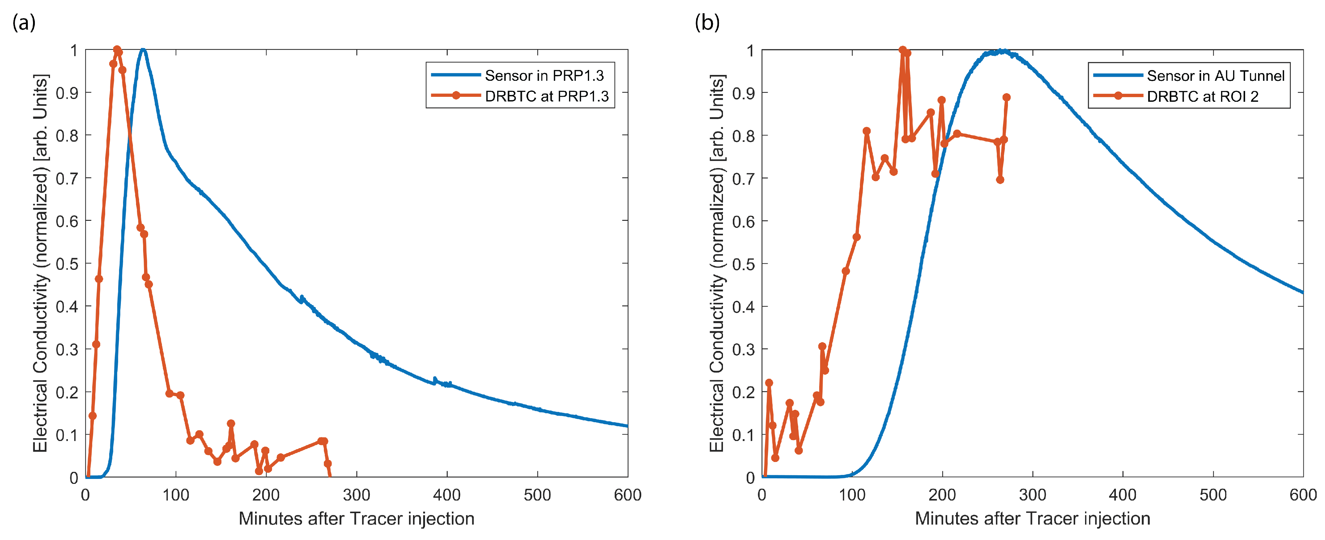
- Experiment 1
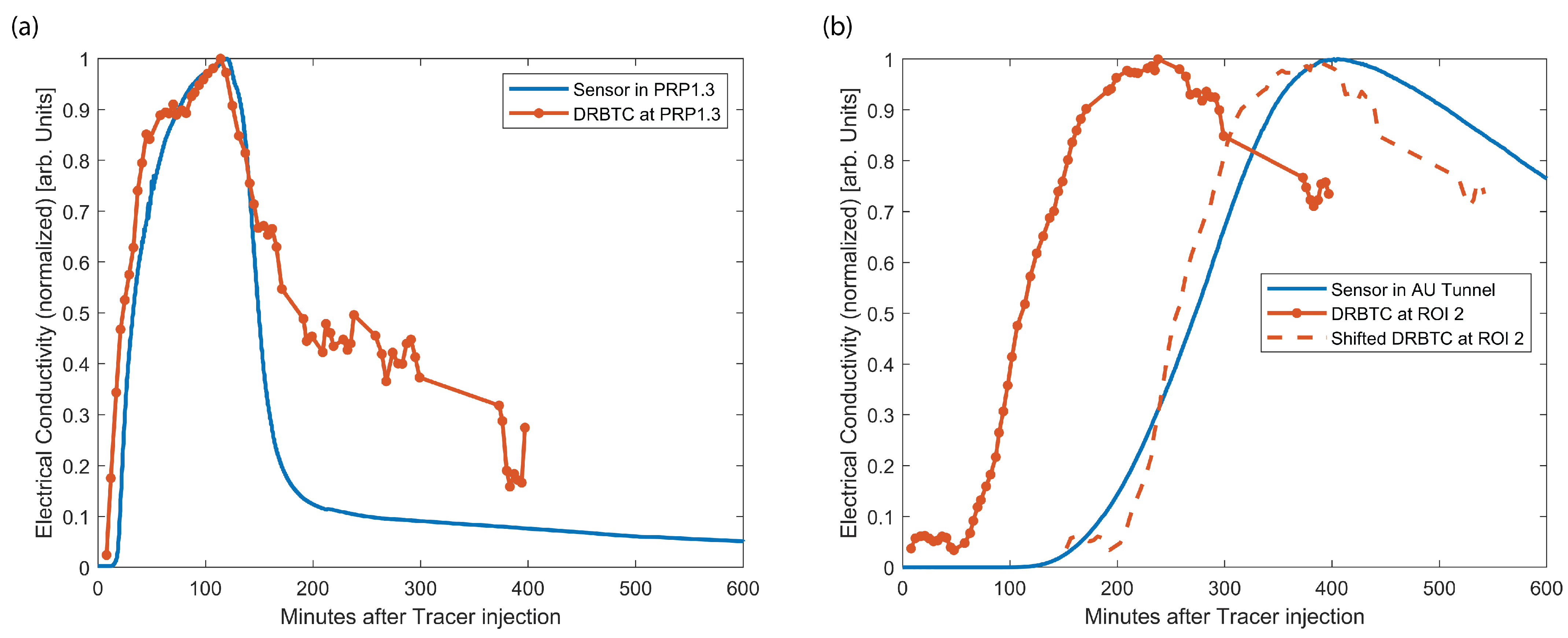
- Experiment 2
3.5. Average Flow Path Velocity Distribution
4. Discussion
4.1. Breakthrough Curves from Difference Reflection Imaging
4.1.1. Difference Radar Breakthrough Curves
4.1.2. DRBTC Limitations
4.1.3. The Importance of Differencing in Field Data
4.2. Average Flow Path Velocity Distribution
4.3. Implications for Geothermal Reservoir Characterization
5. Conclusions
Author Contributions
Funding
Data Availability Statement
Acknowledgments
Conflicts of Interest
Abbreviations
| dielectric permittivity | |
| electrical conductivity | |
| electric field | |
| t | time |
| BTC | breakthrough curve |
| DRBTC | difference radar breakthrough curve |
| GEO | geophysical monitoring borehole |
| GPR | ground penetrating radar |
| GTS | Grimsel Test Site |
| INJ | injection borehole |
| ISC | In-situ Stimulation and Circulation |
| NAGRA | National Cooperative for the Disposal of Radioactive Waste |
| PRP | pressure monitoring borehole |
| RMS | root mean square |
| ROI | region of interest |
| SBH | stress monitoring borehole |
| SNR | signal to noise ratio |
References
- Leibundgut, C.; Maloszewski, P.; Külls, C. Tracers in Hydrology; Wiley-Blackwell: Chichester, UK; Hoboken, NJ, USA, 2009. [Google Scholar]
- Becker, M.W.; Shapiro, A.M. Interpreting Tracer Breakthrough Tailing from Different Forced-Gradient Tracer Experiment Configurations in Fractured Bedrock. Water Resour. Res. 2003, 39. [Google Scholar] [CrossRef]
- Chrysikopoulos, C.V. Artificial Tracers for Geothermal Reservoir Studies. Environ. Geol. 1993, 22, 60–70. [Google Scholar] [CrossRef]
- Ayling, B.F.; Hogarth, R.A.; Rose, P.E. Tracer Testing at the Habanero EGS Site, Central Australia. Geothermics 2016, 63, 15–26. [Google Scholar] [CrossRef]
- Kong, X.Z.; Deuber, C.A.; Kittilä, A.; Somogyvári, M.; Mikutis, G.; Bayer, P.; Stark, W.J.; Saar, M.O. Tomographic Reservoir Imaging with DNA-Labeled Silica Nanotracers: The First Field Validation. Environ. Sci. Technol. 2018, 52, 13681–13689. [Google Scholar] [CrossRef]
- Sanjuan, B.; Pinault, J.L.; Rose, P.; Gérard, A.; Brach, M.; Braibant, G.; Crouzet, C.; Foucher, J.C.; Gautier, A.; Touzelet, S. Tracer Testing of the Geothermal Heat Exchanger at Soultz-Sous-Forêts (France) between 2000 and 2005. Geothermics 2006, 35, 622–653. [Google Scholar] [CrossRef]
- Kittilä, A.; Jalali, M.R.; Somogyvári, M.; Evans, K.F.; Saar, M.O.; Kong, X.Z. Characterization of the Effects of Hydraulic Stimulation with Tracer-Based Temporal Moment Analysis and Tomographic Inversion. Geothermics 2020, 86, 101820. [Google Scholar] [CrossRef]
- Kang, P.K.; Borgne, T.L.; Dentz, M.; Bour, O.; Juanes, R. Impact of Velocity Correlation and Distribution on Transport in Fractured Media: Field Evidence and Theoretical Model. Water Resour. Res. 2015, 51, 940–959. [Google Scholar] [CrossRef]
- Le Borgne, T.; Dentz, M.; Carrera, J. Lagrangian Statistical Model for Transport in Highly Heterogeneous Velocity Fields. Phys. Rev. Lett. 2008, 101, 90601. [Google Scholar] [CrossRef]
- Read, T.; Bour, O.; Bense, V.; Borgne, T.L.; Goderniaux, P.; Klepikova, M.V.; Hochreutener, R.; Lavenant, N.; Boschero, V. Characterizing Groundwater Flow and Heat Transport in Fractured Rock Using Fiber-Optic Distributed Temperature Sensing. Geophys. Res. Lett. 2013, 40, 2055–2059. [Google Scholar] [CrossRef]
- Bernardie, J.d.L.; Bour, O.; Borgne, T.L.; Guihéneuf, N.; Chatton, E.; Labasque, T.; Lay, H.L.; Gerard, M.F. Thermal Attenuation and Lag Time in Fractured Rock: Theory and Field Measurements From Joint Heat and Solute Tracer Tests. Water Resour. Res. 2018, 54, 10053–10075. [Google Scholar] [CrossRef]
- Brixel, B.; Klepikova, M.; Jalali, M.R.; Lei, Q.; Roques, C.; Kriestch, H.; Loew, S. Tracking Fluid Flow in Shallow Crustal Fault Zones: 1. Insights From Single-Hole Permeability Estimates. J. Geophys. Res. Solid Earth 2020, 125, e2019JB018200. [Google Scholar] [CrossRef]
- Brixel, B.; Klepikova, M.; Lei, Q.; Roques, C.; Jalali, M.R.; Krietsch, H.; Loew, S. Tracking Fluid Flow in Shallow Crustal Fault Zones: 2. Insights From Cross-Hole Forced Flow Experiments in Damage Zones. J. Geophys. Res. Solid Earth 2020, 125, e2019JB019108. [Google Scholar] [CrossRef]
- Klepikova, M.; Brixel, B.; Jalali, M. Transient Hydraulic Tomography Approach to Characterize Main Flowpaths and Their Connectivity in Fractured Media. Adv. Water Resour. 2020, 136, 103500. [Google Scholar] [CrossRef]
- Jol, H.M. (Ed.) Ground Penetrating Radar: Theory and Applications, 1st ed.; Elsevier Science: Amsterdam, The Netherlands, 2009. [Google Scholar]
- Niva, B.; Olsson, O.; Blümling, P. Grimsel Test Site: Radar Crosshole Tomography with Application to Migration of Saline Tracer through Fracture Zones; Technical Report NTB 88-31; Nagra: Baden, Switzerland, 1988. [Google Scholar]
- Brewster, M.L.; Annan, A.P. Ground-penetrating Radar Monitoring of a Controlled DNAPL Release: 200 MHz Radar. Geophysics 1994, 59, 1211–1221. [Google Scholar] [CrossRef]
- Day-Lewis, F.D.; Lane, J.W.; Harris, J.M.; Gorelick, S.M. Time-Lapse Imaging of Saline-Tracer Transport in Fractured Rock Using Difference-Attenuation Radar Tomography. Water Resour. Res. 2003, 39. [Google Scholar] [CrossRef]
- Talley, J.; Baker, G.S.; Becker, M.W.; Beyrle, N. Four Dimensional Mapping of Tracer Channelization in Subhorizontal Bedrock Fractures Using Surface Ground Penetrating Radar. Geophys. Res. Lett. 2005, 32, L04401. [Google Scholar] [CrossRef]
- Tsoflias, G.P.; Becker, M.W. Ground-Penetrating-Radar Response to Fracture-Fluid Salinity: Why Lower Frequencies Are Favorable for Resolving Salinity Changes. Geophysics 2008, 73, J25–J30. [Google Scholar] [CrossRef]
- Becker, M.W.; Tsoflias, G.P. Comparing Flux-Averaged and Resident Concentration in a Fractured Bedrock Using Ground Penetrating Radar. Water Resour. Res. 2010, 46. [Google Scholar] [CrossRef]
- Dorn, C.; Linde, N.; Le Borgne, T.; Bour, O.; Klepikova, M. Inferring Transport Characteristics in a Fractured Rock Aquifer by Combining Single-Hole Ground-Penetrating Radar Reflection Monitoring and Tracer Test Data. Water Resour. Res. 2012, 48. [Google Scholar] [CrossRef]
- Allroggen, N.; Tronicke, J. Attribute-Based Analysis of Time-Lapse Ground-Penetrating Radar Data. Geophysics 2016, 81, H1–H8. [Google Scholar] [CrossRef]
- Allroggen, N.; Beiter, D.; Tronicke, J. Ground-Penetrating Radar Monitoring of Fast Subsurface Processes. Geophysics 2020, 85, A19–A23. [Google Scholar] [CrossRef]
- Hawkins, A.J.; Becker, M.W.; Tsoflias, G.P. Evaluation of Inert Tracers in a Bedrock Fracture Using Ground Penetrating Radar and Thermal Sensors. Geothermics 2017, 67, 86–94. [Google Scholar] [CrossRef]
- Shakas, A.; Linde, N.; Baron, L.; Bochet, O.; Bour, O.; Le Borgne, T. Hydrogeophysical Characterization of Transport Processes in Fractured Rock by Combining Push-Pull and Single-Hole Ground Penetrating Radar Experiments. Water Resour. Res. 2016, 52, 938–953. [Google Scholar] [CrossRef]
- Shakas, A.; Linde, N. Apparent Apertures from Ground Penetrating Radar Data and Their Relation to Heterogeneous Aperture Fields. Geophys. J. Int. 2017, 209, 1418–1430. [Google Scholar] [CrossRef]
- Shakas, A.; Linde, N.; Le Borgne, T.; Bour, O. Probabilistic Inference of Fracture-Scale Flow Paths and Aperture Distribution from Hydrogeophysically-Monitored Tracer Tests. J. Hydrol. 2018, 567, 305–319. [Google Scholar] [CrossRef]
- Shakas, A.; Linde, N.; Baron, L.; Selker, J.; Gerard, M.F.; Lavenant, N.; Bour, O.; Le Borgne, T. Neutrally Buoyant Tracers in Hydrogeophysics: Field Demonstration in Fractured Rock. Geophys. Res. Lett. 2017, 44, 3663–3671. [Google Scholar] [CrossRef]
- Giertzuch, P.L.; Doetsch, J.; Jalali, M.; Shakas, A.; Schmelzbach, C.; Maurer, H. Time-Lapse Ground Penetrating Radar Difference Reflection Imaging of Saline Tracer Flow in Fractured Rock. Geophysics 2020, 85, H25–H37. [Google Scholar] [CrossRef]
- Giertzuch, P.L.; Doetsch, J.; Shakas, A.; Jalali, M.; Brixel, B.; Maurer, H. 4D Tracer Flow Reconstruction in Fractured Rock through Borehole GPR Monitoring. Solid Earth Discuss. 2021, 1–27. [Google Scholar] [CrossRef]
- Doetsch, J.; Gischig, V.; Krietsch, H.; Villiger, L.; Amann, F.; Dutler, N.; Jalali, R.; Brixel, B.; Klepikova, M.; Roques, C.; et al. Grimsel ISC Experiment Description; Report; ETH Zurich: Zurich, Switzerland, 2018. [Google Scholar] [CrossRef]
- Amann, F.; Gischig, V.; Evans, K.; Doetsch, J.; Jalali, R.; Valley, B.; Krietsch, H.; Dutler, N.; Villiger, L.; Brixel, B.; et al. The Seismo-Hydromechanical Behavior during Deep Geothermal Reservoir Stimulations: Open Questions Tackled in a Decameter-Scale in Situ Stimulation Experiment. Solid Earth 2018, 9, 115–137. [Google Scholar] [CrossRef]
- Deparis, J.; Garambois, S. On the Use of Dispersive APVO GPR Curves for Thin-Bed Properties Estimation: Theory and Application to Fracture Characterization. Geophysics 2009, 74, J1–J12. [Google Scholar] [CrossRef]
- Shakas, A.; Linde, N. Effective Modeling of Ground Penetrating Radar in Fractured Media Using Analytic Solutions for Propagation, Thin-Bed Interaction and Dipolar Scattering. J. Appl. Geophys. 2015, 116, 206–214. [Google Scholar] [CrossRef]
- Dorn, C.; Linde, N.; Le Borgne, T.; Bour, O.; Baron, L. Single-Hole GPR Reflection Imaging of Solute Transport in a Granitic Aquifer. Geophys. Res. Lett. 2011, 38. [Google Scholar] [CrossRef][Green Version]
- Aldridge, D.F.; Oldenburg, D.W. Refractor Imaging Using an Automated Wavefront Reconstruction Method. Geophysics 1992, 57, 378–385. [Google Scholar] [CrossRef][Green Version]
- Krietsch, H.; Doetsch, J.; Dutler, N.; Jalali, M.; Gischig, V.; Loew, S.; Amann, F. Comprehensive Geological Dataset Describing a Crystalline Rock Mass for Hydraulic Stimulation Experiments. Sci. Data 2018, 5, 180269. [Google Scholar] [CrossRef]
- Doetsch, J.; Krietsch, H.; Schmelzbach, C.; Jalali, M.; Gischig, V.; Villiger, L.; Amann, F.; Maurer, H. Characterizing a Decametre-Scale Granitic Reservoir Using Ground-Penetrating Radar and Seismic Methods. Solid Earth 2020, 11, 1441–1455. [Google Scholar] [CrossRef]
- Brixel, B.; Klepikova, M.; Jalali, M.; Amann, F.; Loew, S. High-Resolution Cross-Borehole Thermal Tracer Testing in Granite: Preliminary Field Results. EGU Gen. Assem. 2017, 2017, 19. [Google Scholar]
- Jalali, M.; Gischig, V.; Doetsch, J.; Näf, R.; Krietsch, H.; Klepikova, M.; Amann, F.; Giardini, D. Transmissivity Changes and Microseismicity Induced by Small-Scale Hydraulic Fracturing Tests in Crystalline Rock. Geophys. Res. Lett. 2018, 45, 2265–2273. [Google Scholar] [CrossRef]
- Kittilä, A.; Jalali, M.R.; Evans, K.F.; Willmann, M.; Saar, M.O.; Kong, X.Z. Field Comparison of DNA-Labeled Nanoparticle and Solute Tracer Transport in a Fractured Crystalline Rock. Water Resour. Res. 2019, 55, 6577–6595. [Google Scholar] [CrossRef]
- Kittilä, A.; Jalali, M.; Saar, M.O.; Kong, X.Z. Solute Tracer Test Quantification of the Effects of Hot Water Injection into Hydraulically Stimulated Crystalline Rock. Geotherm. Energy 2020, 8, 17. [Google Scholar] [CrossRef]
- Jalali, M.; Klepikova, M.; Doetsch, J.; Krietsch, H.; Brixel, B.; Dutler, N.; Gischig, V.; Amann, F. A Multi-Scale Approach to Identify and Characterize the Preferential Flow Paths of a Fractured Crystalline Rock. In Proceedings of the 2nd International Discrete Fracture Network Engineering Conference, Seattle, WA, USA, 20–22 June 2018. [Google Scholar]
- Jalali, R.; Roques, C.; Leresche, S.; Brixel, B.; Giertzuch, P.L.; Doetsch, J.; Schopper, F.; Dutler, N.; Villiger, L.; Krietsch, H.; et al. Evolution of Preferential Flow Paths during the In-Situ Stimulation and Circulation (ISC) Experiment – Grimsel Test Site. Geophys. Res. Abstr. Copernic. 2019, 21. [Google Scholar] [CrossRef]
- Becker, M.W.; Shapiro, A.M. Tracer Transport in Fractured Crystalline Rock: Evidence of Nondiffusive Breakthrough Tailing. Water Resour. Res. 2000, 36, 1677–1686. [Google Scholar] [CrossRef]
- Cherubini, C.; Giasi, C.I.; Pastore, N. On the Reliability of Analytical Models to Predict Solute Transport in a Fracture Network. Hydrol. Earth Syst. Sci. 2014, 18, 2359–2374. [Google Scholar] [CrossRef]
- Dorn, C.; Linde, N.; Doetsch, J.; Le Borgne, T.; Bour, O. Fracture Imaging within a Granitic Rock Aquifer Using Multiple-Offset Single-Hole and Cross-Hole GPR Reflection Data. J. Appl. Geophys. 2012, 78, 123–132. [Google Scholar] [CrossRef]
- Molron, J.; Linde, N.; Baron, L.; Selroos, J.O.; Darcel, C.; Davy, P. Which Fractures Are Imaged with Ground Penetrating Radar? Results from an Experiment in the Äspö Hardrock Laboratory, Sweden. Eng. Geol. 2020, 273, 105674. [Google Scholar] [CrossRef]
- Slob, E.; Sato, M.; Olhoeft, G. Surface and Borehole Ground-Penetrating-Radar Developments. Geophysics 2010, 75, 75A103–75A120. [Google Scholar] [CrossRef]
- Shook, G.M.; Forsmann, J.H. Tracer Interpretation Using Temporal Moments on a Spreadsheet; Technical Report INL/EXT-05-00400, 910998; Idaho National Laboratory (INL): Idaho Falls, ID, USA, 2005. [Google Scholar] [CrossRef]
- Shook, G.M.; Suzuki, A. Use of Tracers and Temperature to Estimate Fracture Surface Area for EGS Reservoirs. Geothermics 2017, 67, 40–47. [Google Scholar] [CrossRef]
- Frieg, B.; Blaser, P.C. Excavation Disturbed Zone Experiment (EDZ); Technical Report 98-01; Nagra: Wettingen, Switzerland, 2012. [Google Scholar]
- Gischig, V.S.; Giardini, D.; Amann, F.; Hertrich, M.; Krietsch, H.; Loew, S.; Maurer, H.; Villiger, L.; Wiemer, S.; Bethmann, F.; et al. Hydraulic Stimulation and Fluid Circulation Experiments in Underground Laboratories: Stepping up the Scale towards Engineered Geothermal Systems. Geomech. Energy Environ. 2020, 24, 100175. [Google Scholar] [CrossRef]
- Shakas, A.; Maurer, H.; Giertzuch, P.L.; Hertrich, M.; Giardini, D.; Serbeto, F.; Meier, P. Permeability Enhancement From a Hydraulic Stimulation Imaged With Ground Penetrating Radar. Geophys. Res. Lett. 2020, 47. [Google Scholar] [CrossRef]


Publisher’s Note: MDPI stays neutral with regard to jurisdictional claims in published maps and institutional affiliations. |
© 2021 by the authors. Licensee MDPI, Basel, Switzerland. This article is an open access article distributed under the terms and conditions of the Creative Commons Attribution (CC BY) license (https://creativecommons.org/licenses/by/4.0/).
Share and Cite
Giertzuch, P.-L.; Shakas, A.; Doetsch, J.; Brixel, B.; Jalali, M.; Maurer, H. Computing Localized Breakthrough Curves and Velocities of Saline Tracer from Ground Penetrating Radar Monitoring Experiments in Fractured Rock. Energies 2021, 14, 2949. https://doi.org/10.3390/en14102949
Giertzuch P-L, Shakas A, Doetsch J, Brixel B, Jalali M, Maurer H. Computing Localized Breakthrough Curves and Velocities of Saline Tracer from Ground Penetrating Radar Monitoring Experiments in Fractured Rock. Energies. 2021; 14(10):2949. https://doi.org/10.3390/en14102949
Chicago/Turabian StyleGiertzuch, Peter-Lasse, Alexis Shakas, Joseph Doetsch, Bernard Brixel, Mohammadreza Jalali, and Hansruedi Maurer. 2021. "Computing Localized Breakthrough Curves and Velocities of Saline Tracer from Ground Penetrating Radar Monitoring Experiments in Fractured Rock" Energies 14, no. 10: 2949. https://doi.org/10.3390/en14102949
APA StyleGiertzuch, P.-L., Shakas, A., Doetsch, J., Brixel, B., Jalali, M., & Maurer, H. (2021). Computing Localized Breakthrough Curves and Velocities of Saline Tracer from Ground Penetrating Radar Monitoring Experiments in Fractured Rock. Energies, 14(10), 2949. https://doi.org/10.3390/en14102949