
The Significance of the Adaptive Thermal Comfort Practice over the Structure Retrofits to Sustain Indoor Thermal Comfort

 , , ,
, , ,  and
and 
Abstract
1. Introduction
1.1. Thermal Comfort
- The predicted mean vote (PMV) and the predicted percentage dissatisfied (PPD) models, which the International Standardisation Organisation (ISO) and Comité European de Normalisation (CEN) standards have also adopted [11].
- Adaptive thermal comfort models.
1.2. Thermal Comfort and Energy Consumption
2. Materials and Methods
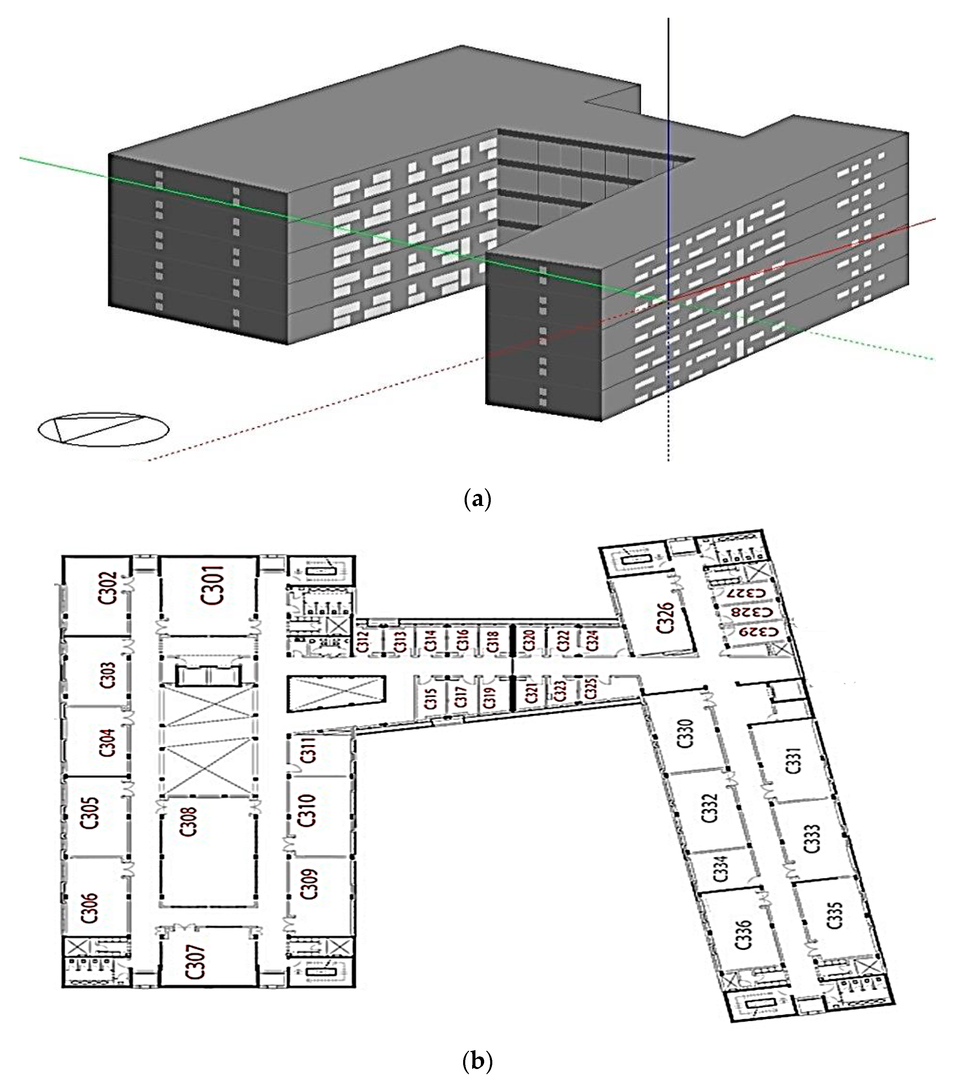
2.1. Location and the Building Characteristics
- The lighting in the building was designed as stated by ASHRAE 90.1 standard.
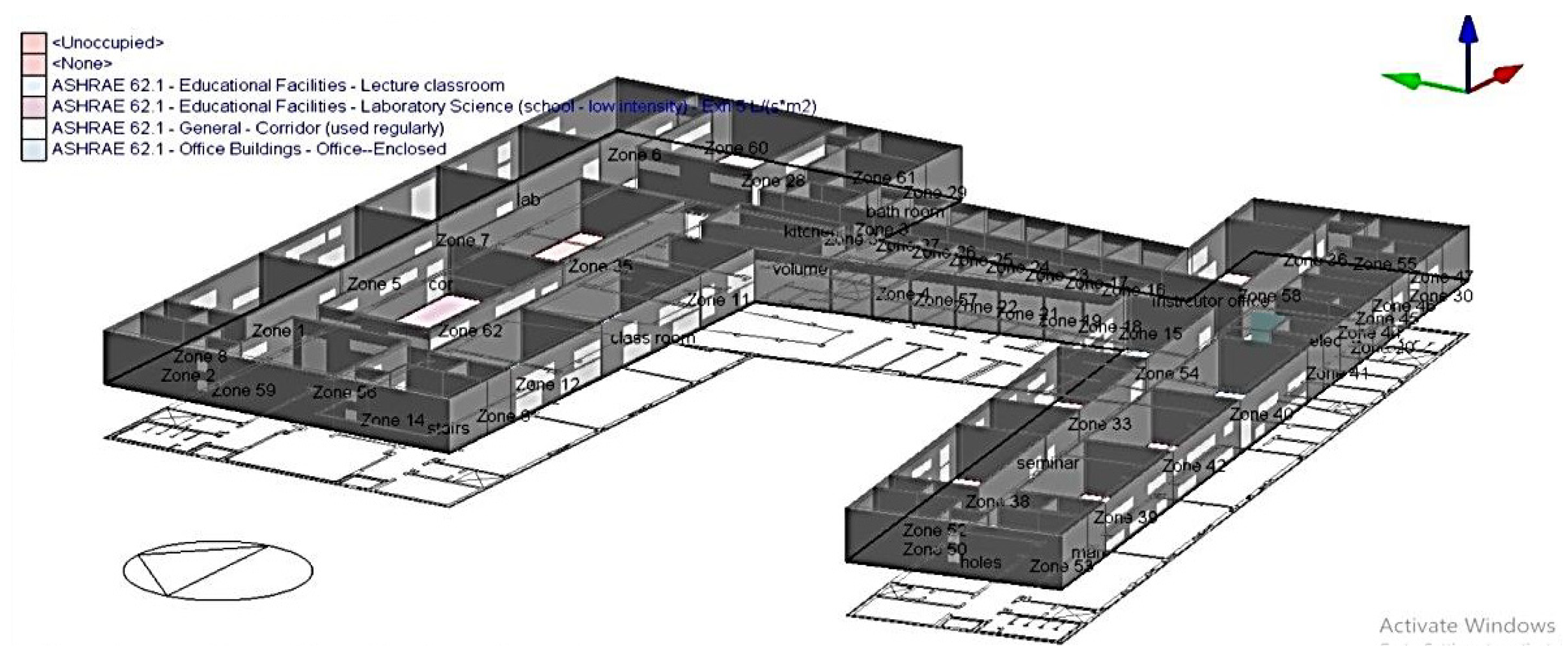
- The building can be divided into 4 thermal zones, which are classrooms, laboratories, offices, and corridors, since the aforesaid utilities are the only thermally conditioned areas of the building. Besides, they almost account for the heaviest energy consumption of the building by themselves.
- The building is supplied with 2 compression chillers with a cooling capacity of 710 kW. One of the chillers also functions as a heat pump. This heat pump is aided by two 200 kW gas boilers that are installed for heating purposes. Moreover, the building is fitted with 3 air handling units to cover its ventilation load.
- The building ventilation load was calculated according to ASHRAE 62.1 standard.
2.2. DesignBuilder Base Building Energy Model (BBEM) Interface
- Introduction of own values: These values could come from either an independent source or automatic calculations done by DesignBuilder.
- Importing a construction from the library: This requires choosing from the lists, including solid (masonry) walls, cavity wall, pitched roof, flat roof, etc. After that, the building regulations which were in effect when the building was constructed, as well as the age bracket into which the building falls, can be selected.
- Inference procedures: These call for the selection of the sector, the building regulations which were in use at the time of construction, and a general description offered by the menus.
2.3. Building Management System (BMS)
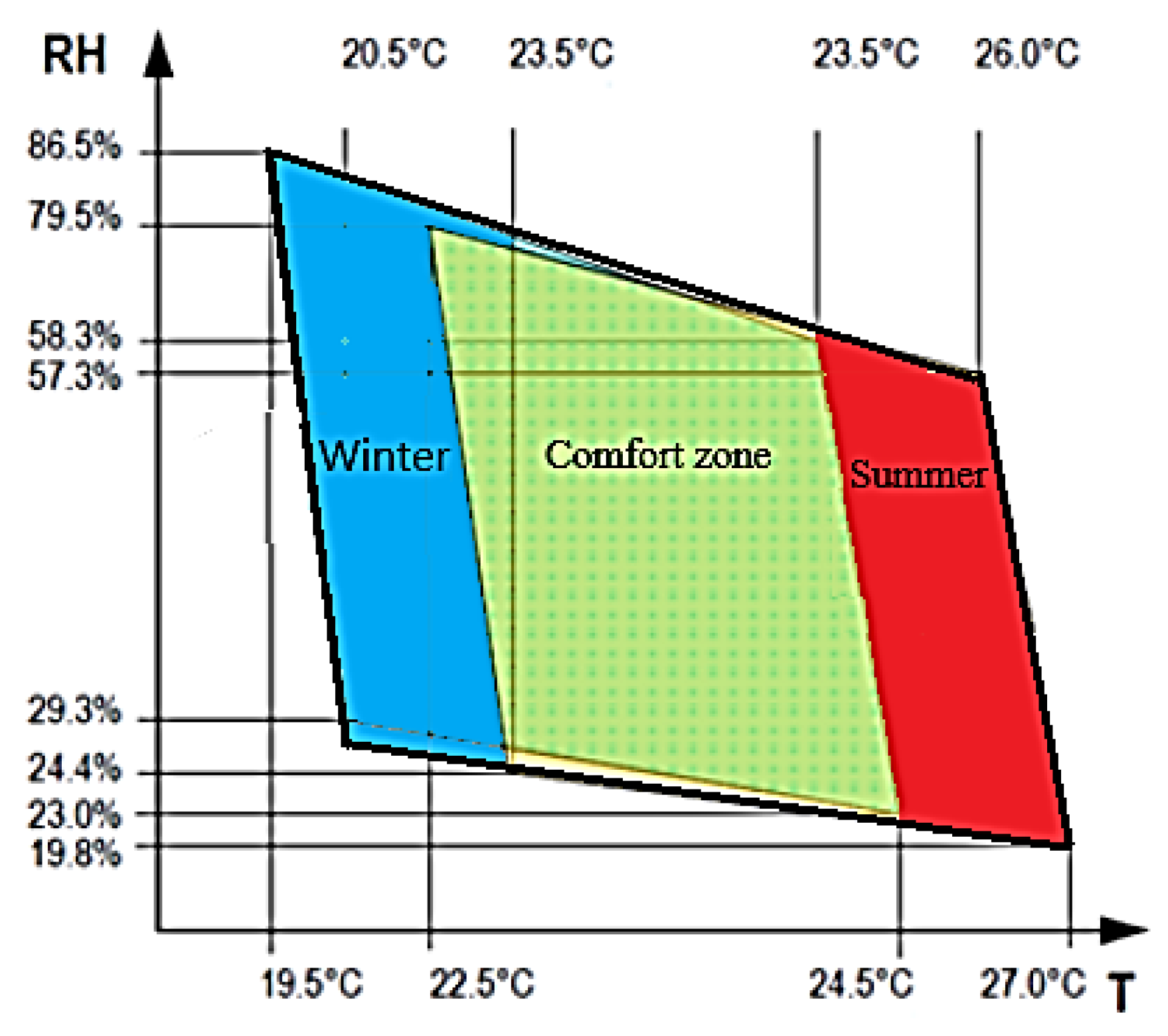
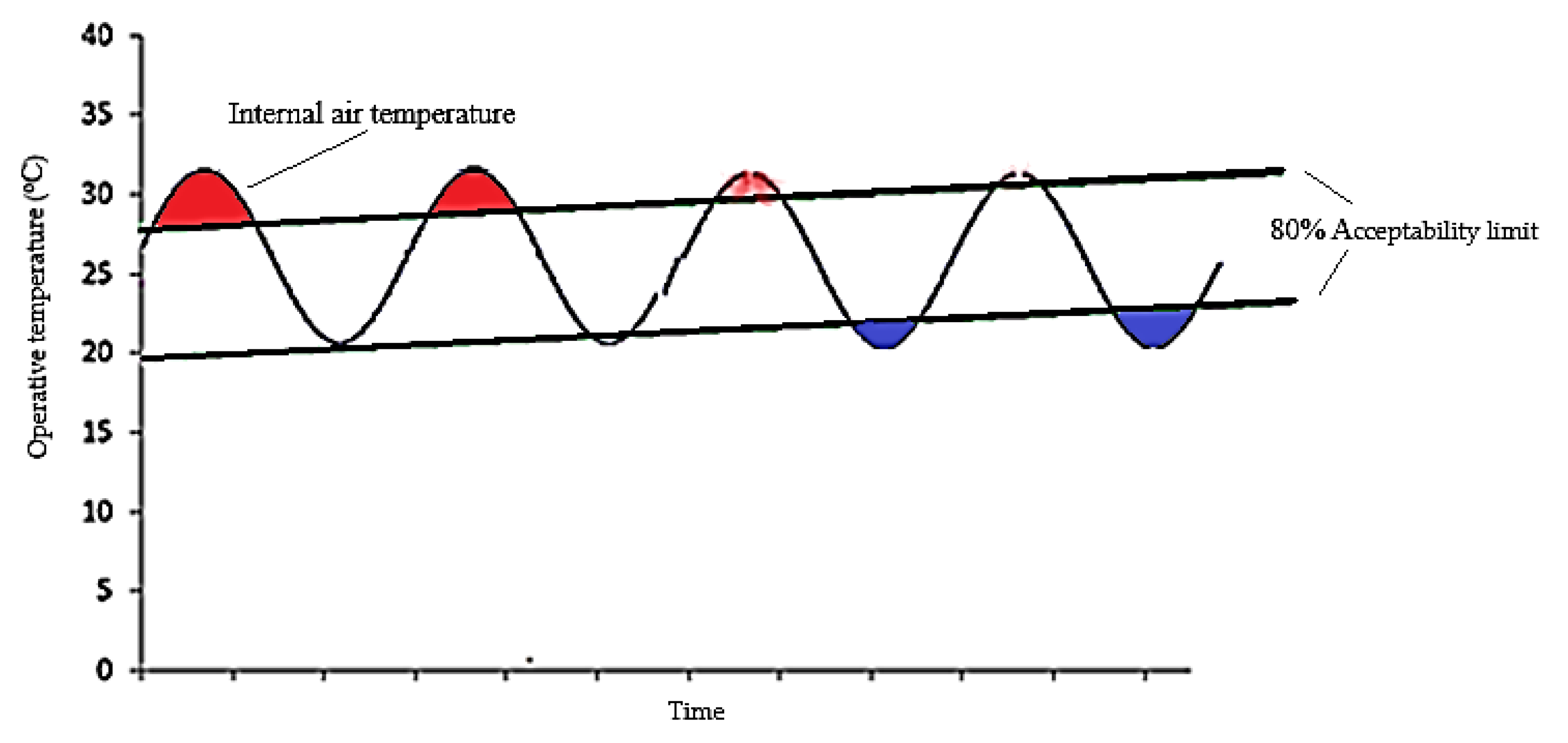
2.4. Thermal Comfort
2.5. Research Methodology (Workflow)
3. Results and Discussion
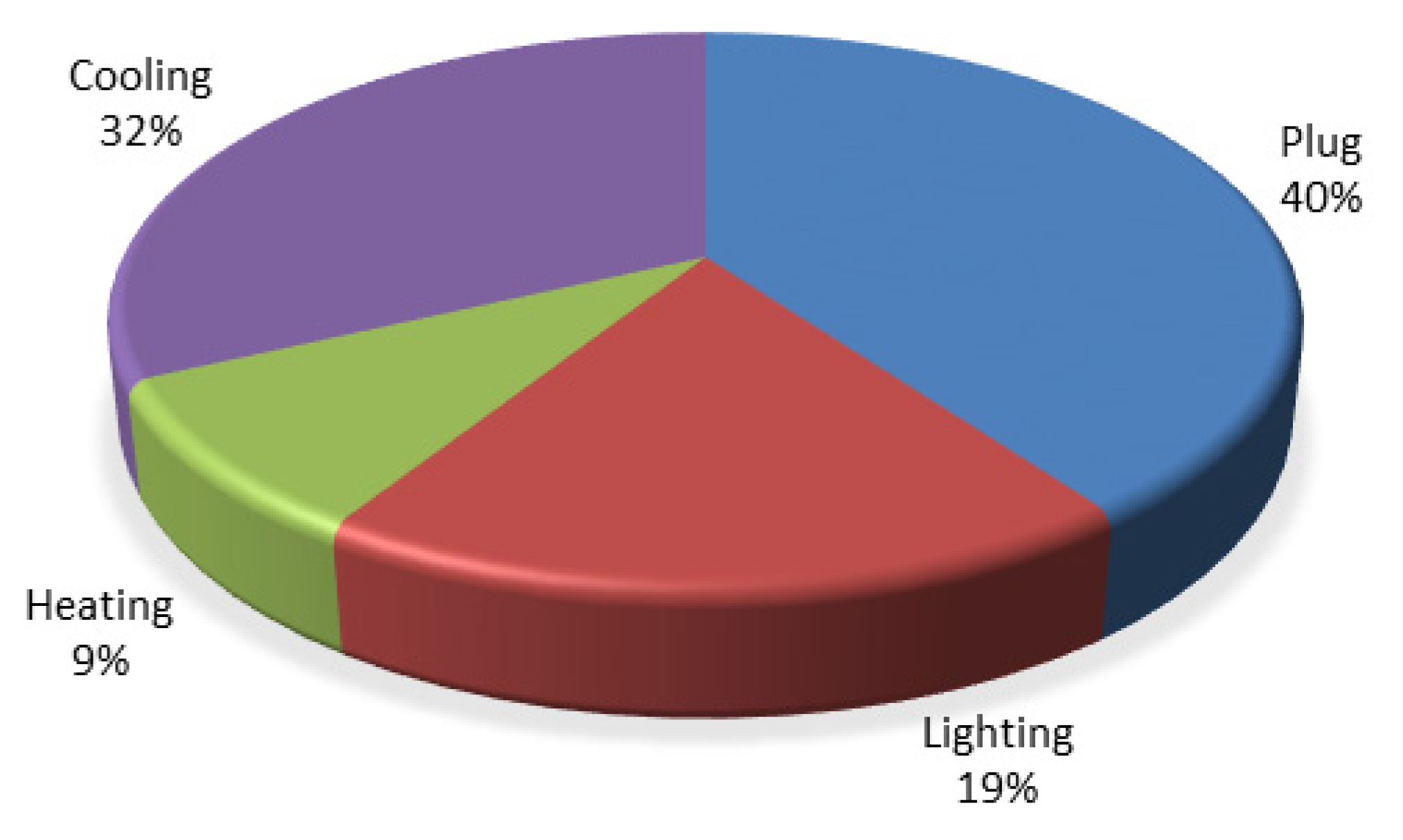
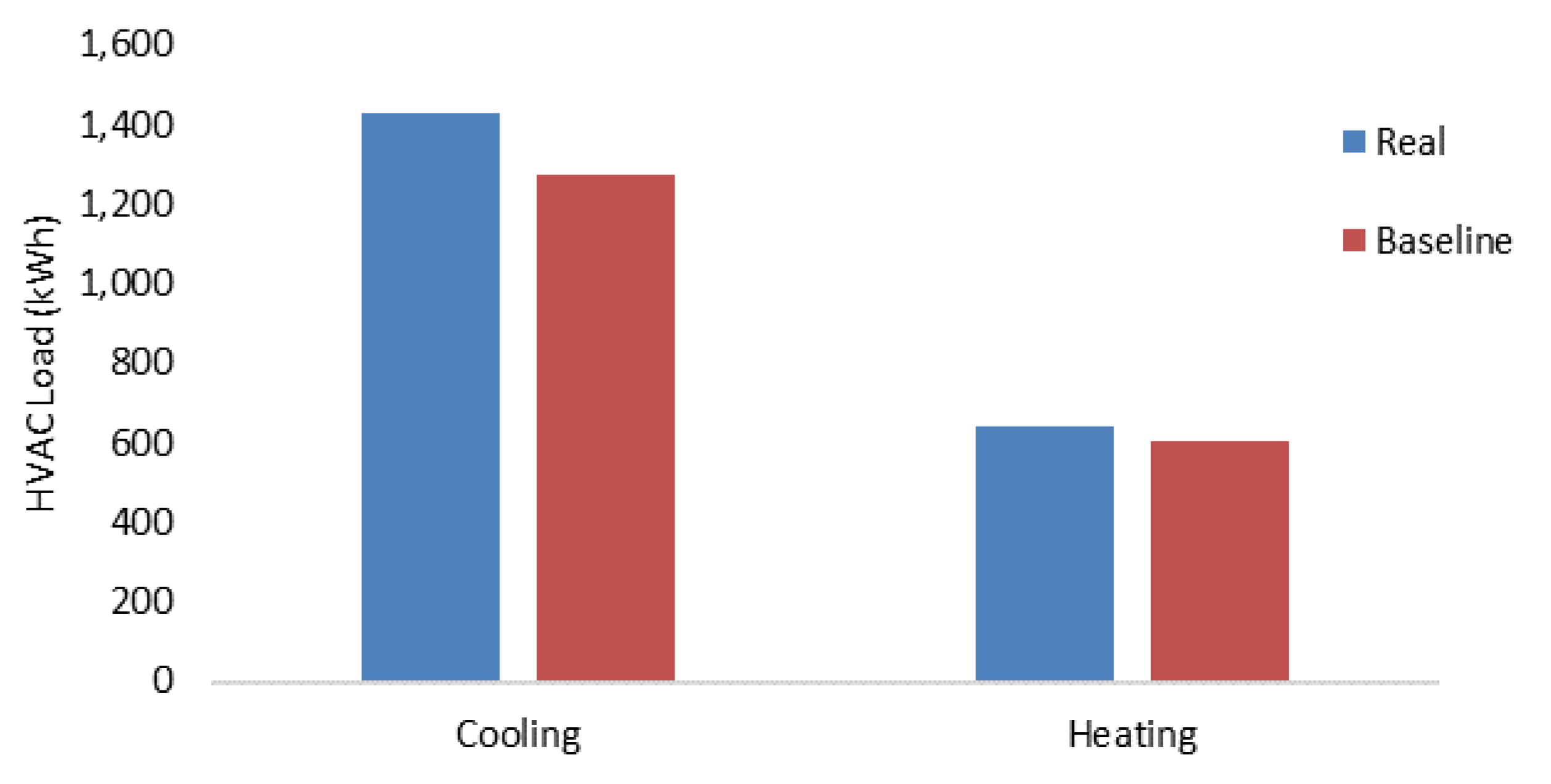
3.1. Baseline Case
3.2. Utilizing LED
3.3. Utilizing Economizers and Heat Recovery
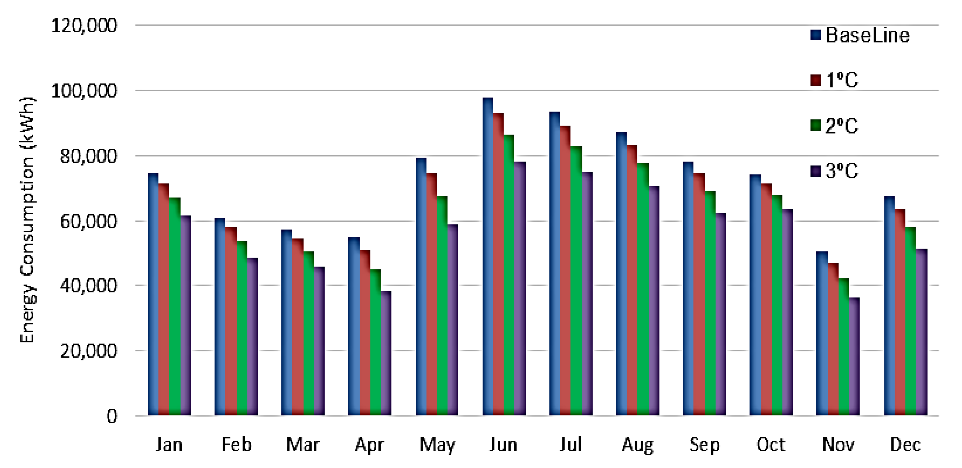
3.4. The Effect of HVAC Set Temperature Points on the Building’s Energy Consumption (Adaptive Limits)
3.5. Summary of the Studied Retrofit Cases
- Wall insulation thickness was increased by 5 cm, 10 cm, 15 cm, and 20 cm to achieve more energy savings. However, the biggest annual energy savings, amounting to 18 MWh/year, were achieved by adding 20 cm walls. However, adding 20 cm walls was too costly, and just increasing the insulation thickness by 5 cm saved around 12.5 MWh/year.
- Roof insulation thickness was increased by 5 cm, 10 cm, and 15 cm to achieve more energy savings. The results show that adding 15 cm insulation roofs led to the biggest annual energy savings, which amounted to 27.9 MWh. In addition, the U-value changed as the roof insulation thickness increased. For practical purposes, 5 cm will be used for this comparison.
- Four different types of glazing were utilized to achieve energy savings. The replacement of the existing glazing by the glaze with a U-value of 1.1W/m2 and solar constant of 0.17 attained 43.2 MWh annual energy savings with a 6-year payback period. Based on this study, it can be concluded that the utilization of triple glazing with higher reflectivity led to the biggest annual energy savings.
- Three kinds of overhangs with varying projection lengths (0.5 cm, 1.0 cm, and 1.5 cm) were employed to achieve energy savings. In conclusion, the employment of 0.5 cm created the greatest annual energy savings, which amounted to 13.3 MWh.
- Three different types of louvers with varying projection lengths (0.5 m, 1 m, and 1.5 m) were used to achieve energy savings. In summary, the use of 1.5 m louvers resulted in the biggest annual energy savings of 16 MWh.
- A simulation of seven different orientations of the building was carried out to conclude the most energy-efficient orientation. The rotation of the building was a hypothetical situation to cover a wide range of scenarios. This simulation shows that the baseline, i.e., the original building’s orientation, was the most energy-efficient, with the least annual energy consumption.
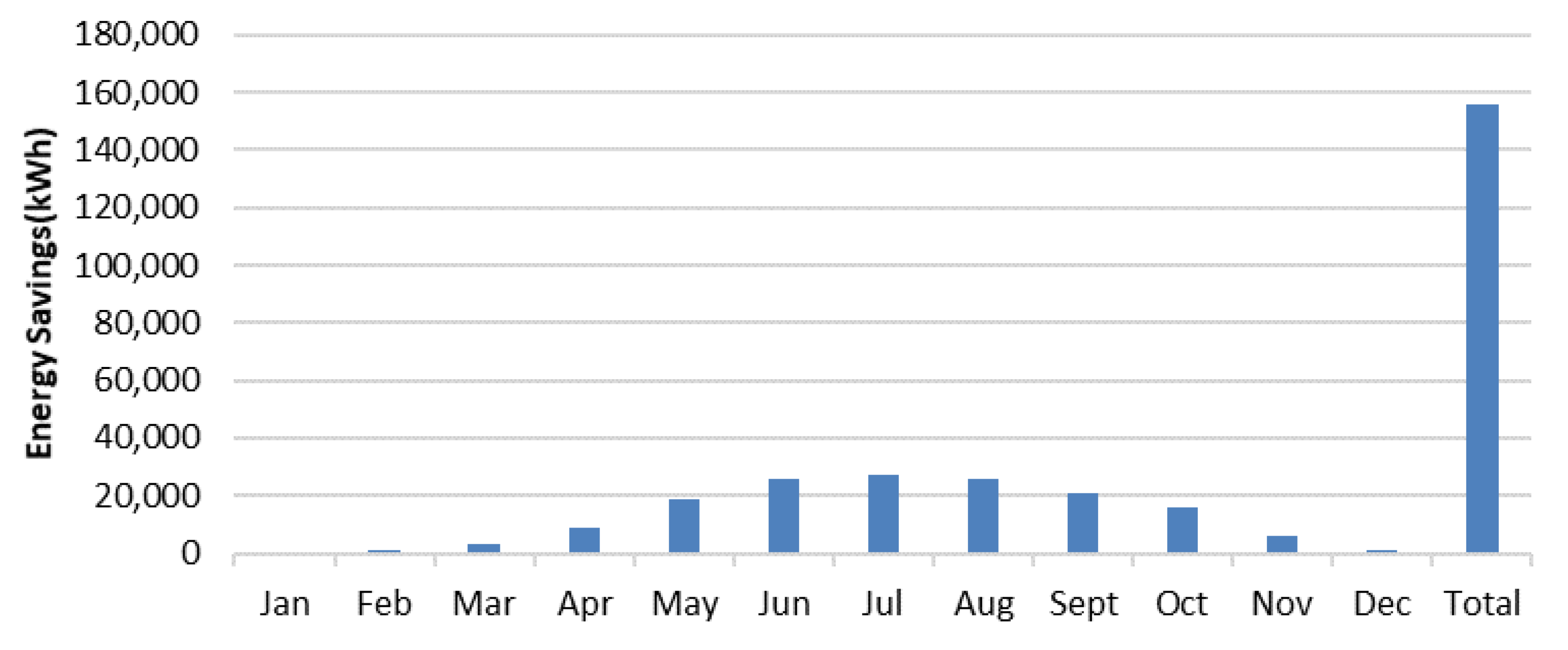
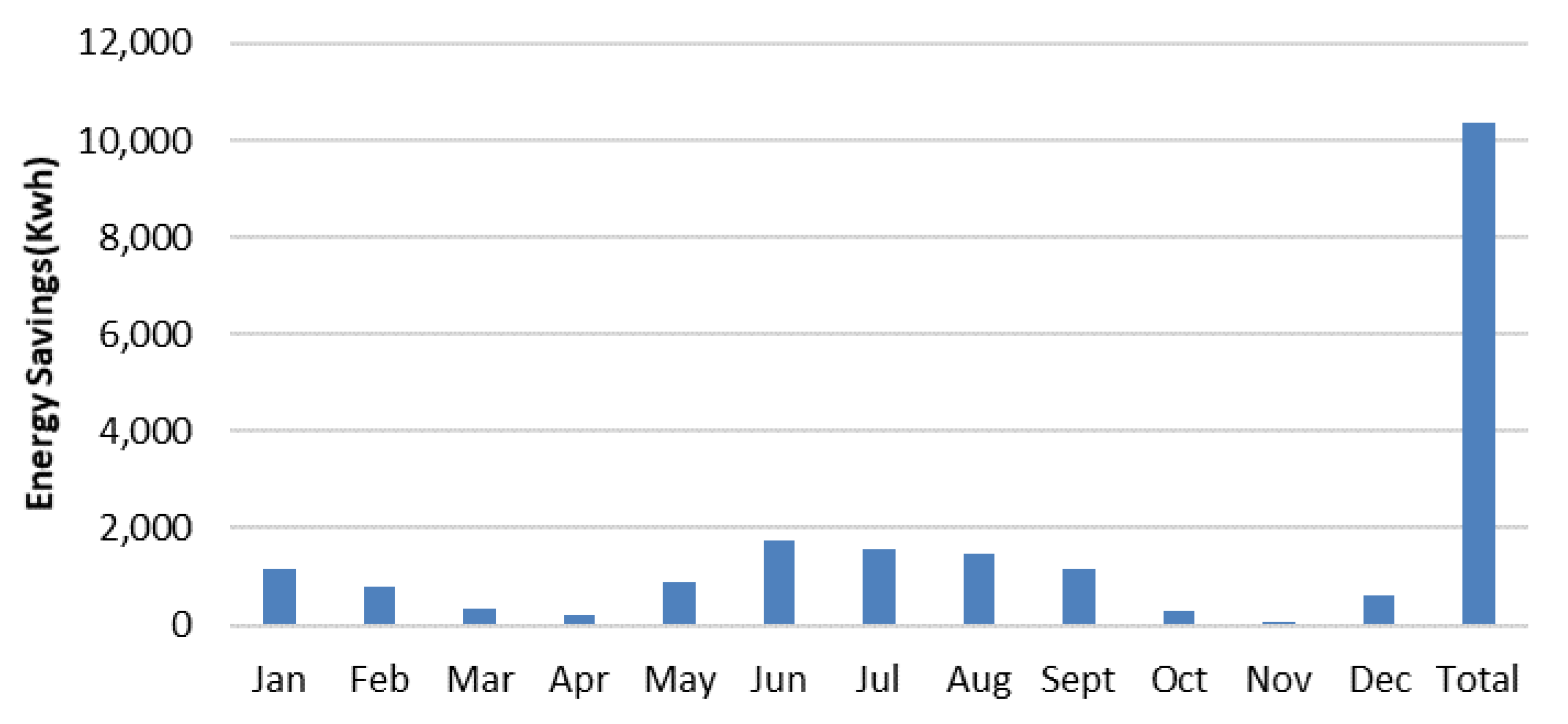
- The economizer and heat recovery unit was utilized to achieve more energy savings. To sum up, energy savings achieved by the economizer were 15-times higher than those made by the heat recovery unit. Whereas the latter achieved 10.4 MWh, the former achieved 156 MWh annual energy savings.
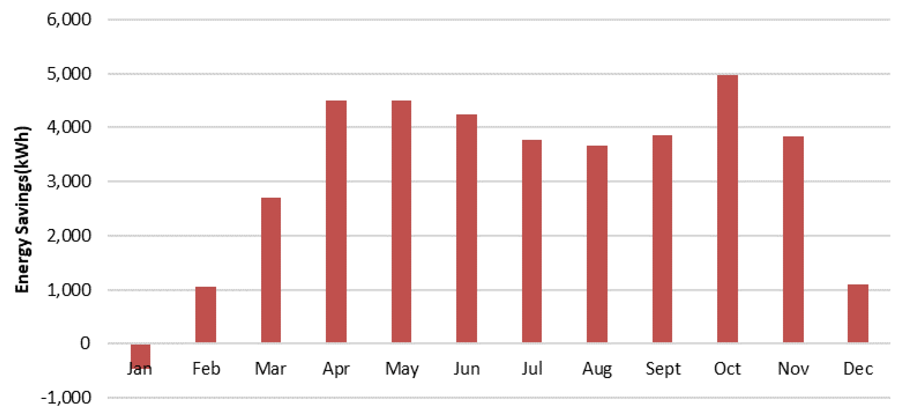
- A simulation in which the building was lit through LED was carried out to determine whether LED lighting saves more energy than conventional lighting. The simulation indicated that LED lighting achieved an annual energy savings of 37.7 MWh.
4. Conclusions
Author Contributions
Funding
Institutional Review Board Statement
Informed Consent Statement
Data Availability Statement
Acknowledgments
Conflicts of Interest
References
- Yang, L.; Yan, H.; Lam, J.C. Thermal comfort and building energy consumption implications—A review. Appl. Energy 2014, 115, 164–173. [Google Scholar] [CrossRef]
- Ministry of Energy and Mineral Resources (MEMR). Annual Report. 2019. Available online: http://www.memr.gov.jo (accessed on 3 February 2021).
- National Electric Power Company (NEPCO). Annual Report. 2018. Available online: http://www.nepco.com.jo (accessed on 3 February 2021).
- Ferreira, P.M.; Ruano, A.E.; Silva, S.; Conceicao, E.Z.E. Neural networks based predictive control for thermal comfort and energy savings in public buildings. Energy Build. 2012, 55, 238–251. [Google Scholar] [CrossRef]
- Alfano, F.R.D.A.; Olesen, B.W.; Palella, B.I.; Riccio, G. Thermal comfort: Design and assessment for energy saving. Energy Build. 2014, 81, 326–336. [Google Scholar] [CrossRef]
- Manzano-Agugliaro, F.; Montoya, F.G.; Sabio-Ortega, A.; García-Cruz, A. Review of bioclimatic architecture strategies for achieving thermal comfort. Renew. Sustain. Energy Rev. 2015, 49, 736–755. [Google Scholar] [CrossRef]
- De Dear, R.; Brager, G.S. Developing an adaptive model of thermal comfort and preference. ASHRAE Tech. Data Bull. 1998, 14, 27–49. [Google Scholar]
- Parsons, K. Human Thermal Environments: The Effects of Hot, Moderate, and Cold Environments on Human Health, Comfort, and Performance; CRC Press: Boca Raton, FL, USA, 2014. [Google Scholar]
- Yun, G.Y. Influences of perceived control on thermal comfort and energy use in buildings. Energy Build. 2018, 158, 822–830. [Google Scholar] [CrossRef]
- American Society of Heating, Refrigerating and Air-Conditioning Engineers (ASHRAE). Thermal Environmental Conditions for Human Occupancy; ANSI/ASHRAE Standard: Peachtree Corners, GA, USA, 2012; pp. 55–2020. [Google Scholar]
- Directive (EU) 2018/844 of the European Parliament and of the Council of 30 May 2018 Amending Directive 2010/31/EU. Available online: https://eur-lex.europa.eu/legal-content/EN/TXT/?uri=uriserv:OJ.L_.2018.156.01.0075.01.ENG&toc=OJ:L:2018:156:FULL (accessed on 29 September 2020).
- Moore, T.; Ridley, I.; Strengers, Y.; Maller, C.; Horne, R. Dwelling performance and adaptive summer comfort in low-income Australian households. Build. Res. Inf. 2017, 45, 443–456. [Google Scholar] [CrossRef]
- Olesen, B.W. Indoor environmental input parameters for the design and assessment of energy performance of buildings. REHVA J. 2015, 52, 17–23. [Google Scholar]
- Mendes, A.; Bonassi, S.; Aguiar, L.; Pereira, C.; Neves, P.; Silva, S.; Teixeira, J.P. Indoor air quality and thermal comfort in elderly care centers. Urban Clim. 2015, 14, 486–501. [Google Scholar] [CrossRef]
- Van Hoof, J. Forty years of Fanger’s model of thermal comfort: Comfort for all? Indoor Air 2008, 18, 182–201. [Google Scholar] [CrossRef]
- d’Ambrosio Alfano, F.R.; Olesen, B.W.; Palella, B.I.; Pepe, D.; Riccio, G. Fifty years of PMV model: Reliability, implementation and design of software for its calculation. Atmosphere 2020, 11, 49. [Google Scholar] [CrossRef]
- Nicol, J.F.; Humphreys, M.A. Adaptive thermal comfort and sustainable thermal standards for buildings. Energy Build. 2002, 34, 563–572. [Google Scholar] [CrossRef]
- Wu, T.; Cao, B.; Zhu, Y. A field study on thermal comfort and air-conditioning energy use in an office building in Guangzhou. Energy Build. 2018, 168, 428–437. [Google Scholar] [CrossRef]
- Mora, R.; Bean, R. Thermal comfort: Designing for people. ASHRAE J. 2018, 60, 40–46. [Google Scholar]
- Newsham, G.R.; Birt, B.J.; Arsenault, C.; Thompson, A.J.; Veitch, J.A.; Mancini, S.; Burns, G.J. Do ‘green’buildings have better indoor environments? New evidence. Build. Res. Inf. 2013, 41, 415–434. [Google Scholar] [CrossRef]
- Guideline 10-2016—Interactions Affecting the Achievement of Acceptable Indoor Environments; American Society of Heating, Refrigerating and Air-Conditioning Engineers (ASHRAE): Atlanta, GA, USA, 2016.
- Soebarto, V.; Bennetts, H. Thermal comfort and occupant responses during summer in a low to middle income housing development in South Australia. Build. Environ. 2014, 75, 19–29. [Google Scholar] [CrossRef]
- De Dear, R.; Brager, G.S. Developing An Adaptive Model of Thermal Comfort and Preference; Indoor Environmental Quality (IEQ) SF-98-7-3 (4106) (RP-884); California Digital Library: Berkeley, CA, USA, 1998. [Google Scholar]
- Nicol, F.; Humphreys, M. Derivation of the adaptive equations for thermal comfort in free-running buildings in European standard EN15251. Build. Environ. 2010, 45, 11–17. [Google Scholar] [CrossRef]
- Ren, Z.; Chen, D. Modelling study of the impact of thermal comfort criteria on housing energy use in Australia. Appl. Energy 2018, 210, 152–166. [Google Scholar] [CrossRef]
- Hwang, R.L.; Lin, T.P.; Kuo, N.J. Field experiments on thermal comfort in campus classrooms in Taiwan. Energy Build. 2016, 38, 53–62. [Google Scholar] [CrossRef]
- Fanger, P.O. The effect of air humidity in buildings on man’s comfort and health. In Proceedings of the CISCO-ITBTP Seminar Humidity in Building, Saint Remy les Chevreuse, France, November 1982. [Google Scholar]
- Fanger, P.O.; Toftum, J. Extension of the PMV model to non-air-conditioned buildings in warm climates. Energy Build. 2002, 34, 533–536. [Google Scholar] [CrossRef]
- Moujalled, B.; Cantin, R.; Guarracino, G. Comparison of thermal comfort algorithms in naturally ventilated office buildings. Energy Build. 2008, 40, 2215–2223. [Google Scholar] [CrossRef]
- Holopainen, R.; Tuomaala, P.; Hernandez, P.; Häkkinen, T.; Piira, K.; Piippo, J. Comfort assessment in the context of sustainable buildings: Comparison of simplified and detailed human thermal sensation methods. Build. Environ. 2014, 71, 60–70. [Google Scholar] [CrossRef]
- Ji, W.; Cao, B.; Luo, M.; Zhu, Y. Influence of short-term thermal experience on thermal comfort evaluations: A climate chamber experiment. Build. Environ. 2017, 114, 246–256. [Google Scholar] [CrossRef]
- Castaño-Rosa, R.; Rodríguez-Jiménez, C.E.; Rubio-Bellido, C. Adaptive thermal comfort potential in mediterranean office buildings: A case study of Torre Sevilla. Sustainability 2018, 10, 3091. [Google Scholar] [CrossRef]
- WheaterOnline.co.uk. Jordan. Available online: https://www.weatheronline.co.uk/reports/climate/Jordan.htm. (accessed on 4 December 2020).
- Thermal Environmental Conditions for Human Occupancy; American Society of Heating, Refrigerating and Air-Conditioning Engineers (ASHRAE): Atlanta, GA, USA, 2013.
- Harvey, L.D.D. A Handbook on Low-Energy Buildings District-Energy Systems: Fundamentals, Techniques and Example; Routledge: London, UK, 2015. [Google Scholar]
- De Dear, R. Developing an adaptive model of thermal comfort and preference, field studies of thermal comfort and adaptation. ASHRAE Tech. Data Bull. 1998, 104, 145–167. [Google Scholar]


| Floor Number | Area (103 m2) | Number of Classrooms | Number of Offices | Number of Laboratories |
|---|---|---|---|---|
| Ground Floor | 1.77 | 0 | 15 | 6 |
| First Floor | 3.32 | 6 | 27 | 7 |
| Second Floor | 2.62 | 10 | 21 | 6 |
| Third Floor | 2.51 | 8 | 19 | 9 |
| Fourth Floor | 2.49 | 0 | 25 | 15 |
| Layer Name | Thermal Conductivity (W/m K) | Thickness (mm) | |
|---|---|---|---|
| External Walls | Stone | 2.2 | 50 |
| Concrete | 1.75 | 200 | |
| Extruded polystyrene | 0.03 | 50 | |
| Concrete Block | 1 | 13 | |
| Cement Plaster | 1.2 | 20 | |
| Overall heat transfer coefficient = 0.469 W/m2 K | |||
| Internal Walls | Cement Plaster | 1.2 | 30 |
| Concrete | 1.75 | 200 | |
| Cement Plaster | 1.2 | 30 | |
| Overall Heat Transfer Coefficient = 1.61 W/m2 K | |||
| Roof Materials | Asphalt | 0.7 | 20 |
| Extruded polystyrene | 0.03 | 59 | |
| Concrete | 1.75 | 75 | |
| Cement Plaster | 1.2 | 20 | |
| Overall Heat Transfer Coefficient = 0.37 W/m2 K | |||
| External Windows Frame Materials | Aluminum | 160 | 2 |
| polyvinyl chloride (pvc) | 0.17 | 5 | |
| Overall Heat Transfer Coefficient = 5.01 W/m2 K. | |||
| Glazing | Glazing Overall Heat Transfer Coefficient = 2.4 W/m2 K Solar Factor = 24% | ||
| Room Type | Lighting Power Density (Lux) | Ventilation Rate (Liter/Second) Per Person |
|---|---|---|
| Class Room | 467 | 3.8 |
| Laboratory | 467 | 5 |
| Office | 400 | 2.5 |
| Corridor | 167 | 0.3 |
| Room Type | Occupancy Density (Person/Room) | Operating Days and Hours |
|---|---|---|
| Class room | 65 | Sunday-Thursday 7:00 a.m.–5:00 p.m. |
| Laboratory | 25 | Sunday-Thursday 10:00 a.m.–5:00 p.m. |
| Office | 5 | Sunday-Thursday 7:00 a.m.–5:00 p.m. |
| Corridor | - | Sunday-Thursday 7:00 a.m.–5:00 p.m. |
| Room Type | Plug Load (W/m2) |
|---|---|
| Class Room | 5 |
| Laboratory | 50 |
| Instructor office | 5 |
| Corridor | 3 |
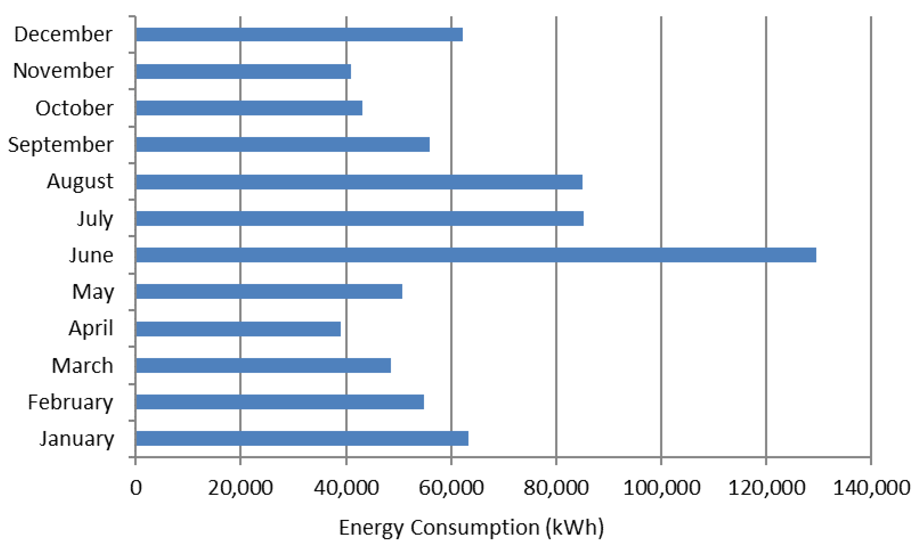
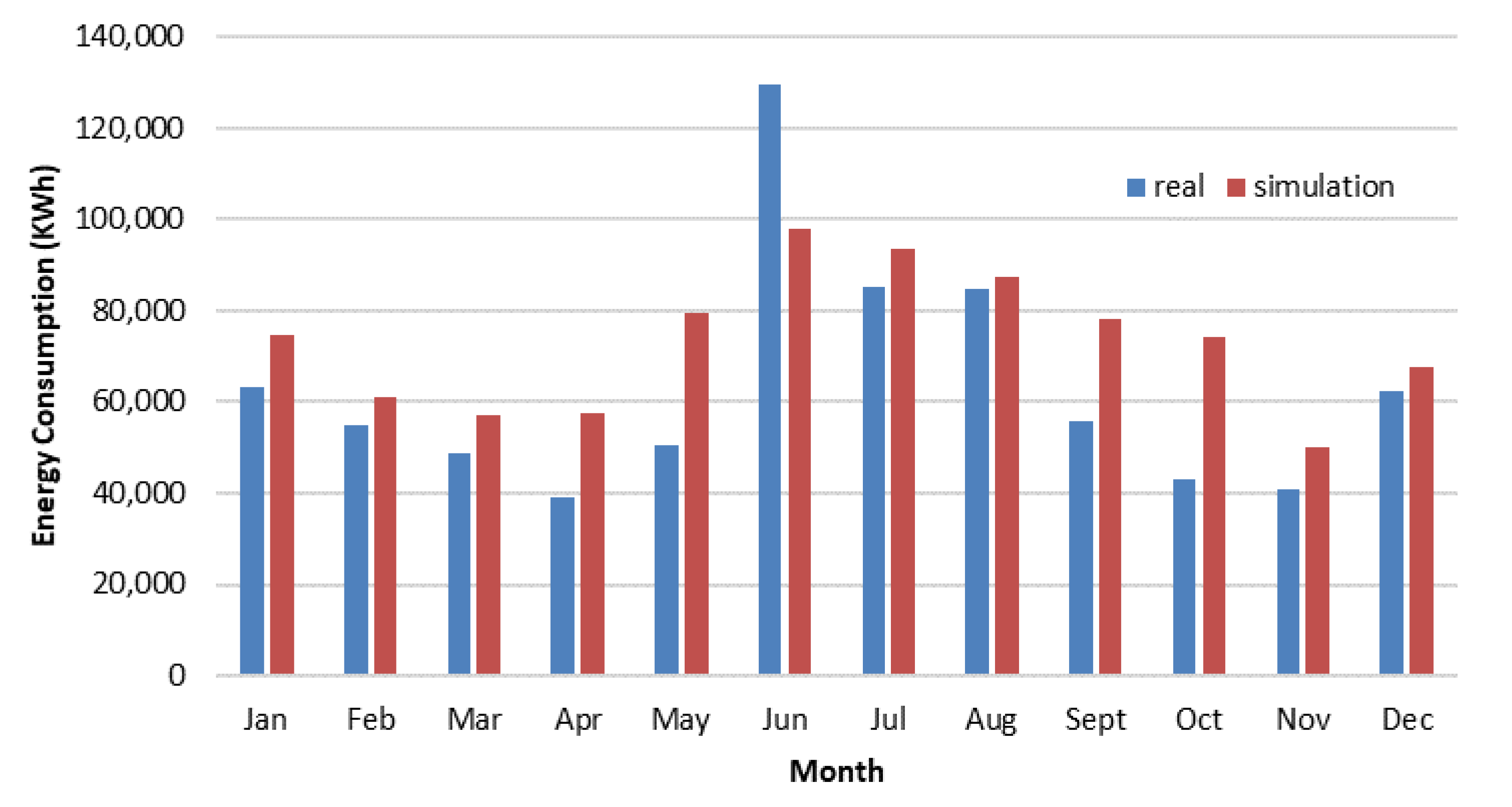
| Month | Energy Consumption (MWh) |
|---|---|
| January | 63.4 |
| February | 54.9 |
| March | 48.6 |
| April | 39 |
| May | 50.7 |
| June | 130 |
| July | 85.1 |
| August | 84.9 |
| September | 55.9 |
| October | 43.1 |
| November | 41 |
| December | 62.3 |
| Component | Heat Recovery | Economizer |
|---|---|---|
| Cost ($USD) | 15 K | 50 K |
| Annual savings ($USD) | 1.03 K | 15.5 K |
| NPV($USD) | −6.6 K | 66.7 K |
| IRR (%) | −6% | 29% |
| PBP (yr) | 27 | 4 |
| Case | Annual Energy Savings (MWh) | Cost |
|---|---|---|
| Increase of wall insulation thickness by 5 cm | 12.5 | High |
| Add 0.5 m projection lengths to the windows | 13.3 | High |
| Add louvers with projection lengths 1.5 m | 16 | High |
| Increasing roof insulation thickness by 5 cm | 22.2 | High |
| Utilization of LED lighting | 37.8 | Low |
| Replacement of glazing by triple glazing | 43.2 | Medium |
| First heating and cooling adaptive scenario (1 °C) | 43.8 | Almost Null |
| Second heating and cooling adaptive scenario (2 °C) | 7.8 | Almost Null |
| Installation of ventilation air economizer | 155 | Medium |
| Third heating and cooling adaptive scenario (3 °C) | 185 | Almost Null |
Publisher’s Note: MDPI stays neutral with regard to jurisdictional claims in published maps and institutional affiliations. |
© 2021 by the authors. Licensee MDPI, Basel, Switzerland. This article is an open access article distributed under the terms and conditions of the Creative Commons Attribution (CC BY) license (https://creativecommons.org/licenses/by/4.0/).
Share and Cite
Albatayneh, A.; Jaradat, M.; AlKhatib, M.B.; Abdallah, R.; Juaidi, A.; Manzano-Agugliaro, F. The Significance of the Adaptive Thermal Comfort Practice over the Structure Retrofits to Sustain Indoor Thermal Comfort. Energies 2021, 14, 2946. https://doi.org/10.3390/en14102946
Albatayneh A, Jaradat M, AlKhatib MB, Abdallah R, Juaidi A, Manzano-Agugliaro F. The Significance of the Adaptive Thermal Comfort Practice over the Structure Retrofits to Sustain Indoor Thermal Comfort. Energies. 2021; 14(10):2946. https://doi.org/10.3390/en14102946
Chicago/Turabian StyleAlbatayneh, Aiman, Mustafa Jaradat, Mhd Bashar AlKhatib, Ramez Abdallah, Adel Juaidi, and Francisco Manzano-Agugliaro. 2021. "The Significance of the Adaptive Thermal Comfort Practice over the Structure Retrofits to Sustain Indoor Thermal Comfort" Energies 14, no. 10: 2946. https://doi.org/10.3390/en14102946
APA StyleAlbatayneh, A., Jaradat, M., AlKhatib, M. B., Abdallah, R., Juaidi, A., & Manzano-Agugliaro, F. (2021). The Significance of the Adaptive Thermal Comfort Practice over the Structure Retrofits to Sustain Indoor Thermal Comfort. Energies, 14(10), 2946. https://doi.org/10.3390/en14102946