Exploring the Potentialities of Deep Reinforcement Learning for Incentive-Based Demand Response in a Cluster of Small Commercial Buildings

Abstract

Demand Response (DR) programs represent an effective way to optimally manage building energy demand while increasing Renewable Energy Sources (RES) integration and grid reliability, helping the decarbonization of the electricity sector. To fully exploit such opportunities, buildings are required to become sources of energy flexibility, adapting their energy demand to meet specific grid requirements. However, in most cases, the energy flexibility of a single building is typically too small to be exploited in the flexibility market, highlighting the necessity to perform analysis at a multiple-building scale. This study explores the economic benefits associated with the implementation of a Reinforcement Learning (RL) control strategy for the participation in an incentive-based demand response program of a cluster of commercial buildings. To this purpose, optimized Rule-Based Control (RBC) strategies are compared with a RL controller. Moreover, a hybrid control strategy exploiting both RBC and RL is proposed. Results show that the RL algorithm outperforms the RBC in reducing the total energy cost, but it is less effective in fulfilling DR requirements. The hybrid controller achieves a reduction in energy consumption and energy costs by respectively 7% and 4% compared to a manually optimized RBC, while fulfilling DR constraints during incentive-based events.

1. Introduction

The path towards the decarbonization of the energy and building sector paved the way for the integration of Renewable Energy Sources (RES), seen as key actors to tackle climate change.

However, the high volatility of renewable electricity sources can jeopardize grid reliability [1]. In this scenario, system flexibility can be exploited to guarantee the stability of the electricity grid [2]. Energy flexibility can be provided by three main sources: flexible generators (e.g., cogeneration units), energy storages (e.g., batteries, thermal storages), and flexible demand (e.g., industrial or commercial buildings) [2].

However, due to the high cost of operating and maintaining flexible sources on the supply-side [3], the last few years have seen building Demand Side Flexibility (DSF) as one of the most explored and promising opportunities. In fact, buildings account for around 40% of global energy demand, thus representing a valuable opportunity for the design of advanced strategies oriented to provide demand flexibility services. According to [4], the energy flexibility of a building depends on the possibility to manage its energy demand and local generation according to climate conditions, user needs, and grid requirements. 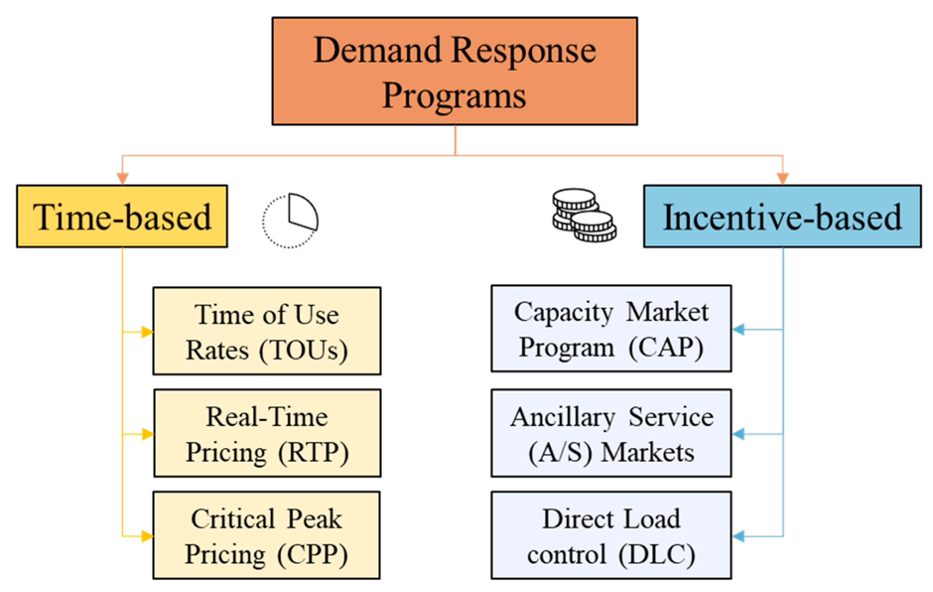This can be achieved by implementing Demand Side Management (DSM) [5] and load control strategies, which also include Demand Response (DR) programs [6]. DR programs allow users to obtain an economic advantage from the curtailment or shifting of their building load according to the grid requirements, and they can be classified into two main categories, as shown in Figure 1: incentive-based and time-based programs [7].

The incentive-based DR relies on remuneration of participants who manually or automatically reduced their electrical loads after a request delivered from the DR service provider thanks to the adoption of Capacity Market Program (CAP) (e.g., aggregator), or allowing the provider to turn off some appliances, as in Direct Load Control (DLC) programs. This kind of DR program is beneficial to address temporary unfavorable conditions, such as local or regional grid congestion or operational reliability problems, such as Ancillary Services (A/S). On the other hand, time-based DR programs leverage the use of dynamic energy prices that can be established in advance, as Time of Use rates (TOUs), in Real-Time (RTP), or according to grid necessities (e.g., Critical Peak Pricing (CPP)). Such tariffs are used to incentivize energy users to shift their electrical energy consumption from peak to off-peak hours.

The following subsection provides an overview of DR-related works, together with adopted control strategies and paper contributions.

Related Works

Many studies have analyzed the role and potentialities of demand response in buildings, highlighting the potential benefits for the grid. Early studies analyzed the role of curtailable loads, such as smart appliances and smart lighting systems, which can be controlled by the Building Energy Management System (BEMS) [8], considering user preferences [9,10] to minimize energy consumption [11,12]. Other studies have discussed the application of DR-oriented strategies considering the management of energy systems, such as electric heaters [13] and energy storage technologies [14,15], to facilitate the participation in DR programs for residential and small commercial customers. In addition, as stated in [16], the increasing spread of Electric Vehicles (EV) and Hybrid Electric Vehicles (HEV) has introduced the opportunity to exploit the management of EV charge/discharge cycles [17,18] for providing peak shaving [19,20] and ancillary services [21,22] to the grid.

Lastly, many studies have focused the attention on HVAC systems that could be responsible up to 50% of electricity consumption in commercial buildings. From this perspective, the optimal management of HVAC systems represents a significant flexibility resource for the electrical grid, as extensively documented in [23,24,25,26], that can bring benefits in terms of peak reduction and frequency regulation [27,28]. However, the participation in DR events leveraging HVAC systems bears the risk of Indoor Environmental Quality (IEQ) and comfort degradation for building occupants. Indeed, despite the great potential in terms of demand flexibility, the spread of DR programs in small commercial buildings has still to overcome some barriers to unlock its full potential without impacting user preferences, since electricity is a resource whose value for consumers is much higher than its price [29]. Specifically, to avoid indoor thermal comfort violations while participating in DR events, thermal storages play a key role [30], making it possible to fully unlock the energy flexibility potential of buildings minimizing the compromises for the occupants. For this reason, recent studies have investigated the effectiveness of control strategies for increasing the feasibility of DR programs by means of optimized management of thermal storage and HVAC systems [31,32].

As highlighted, the future of demand response in buildings will be greatly influenced by the ability of novel control logics in preventing occupant discomfort while ensuring, with an optimized energy system management, technical benefits for the grid and cost savings for end-users. To this purpose, there is an increasing need for advanced approaches to the building control problem that make it possible to consider multiple objective optimizations also including new requirements emerging from the grid side.

In the literature, several methods have been used to deal with DR optimization problems, whose main drivers are the scale of the analysis and the computational requirements. The most used approaches rely on convex optimization methods, such as Mixed Integer Linear Programming (MILP) [33] or Mixed Integer Non-Linear Programming (MILNP) [34], considering the single building scale. Depending on the constraints and complexity of the considered DR problem, other common techniques include fuzzy logic controllers [35] and Particle Swarm Optimization (PSO) [15], achieving near-optimal solutions.

However, when dealing with a multiple-building scale, mathematical solutions require the introduction of a bi-level optimization, increasing the computational complexity of the control problem and limiting the effectiveness of MILP. Among the proposed alternatives, game theory-based algorithms [36], Genetic Algorithms (GA), and learning-based algorithms [37] represent valuable solutions to reduce computational costs while finding near-optimal solutions for large-scale control problems.

In this context, recent studies started to investigate the potentiality of Reinforcement Learning (RL), a branch of machine learning that deals with the optimal control of complex systems [38] for building energy management. One of the main key features of RL is its model-free nature. Indeed, RL algorithms do not require a model of the system to be controlled and learn a sub-optimal control policy through trial-and-error interaction with the environment and by leveraging historical data. This feature allows RL controllers to integrate human preferences into the control loop, making them suitable for the control of complex energy systems that deal with non-linearity processes [39] and demand response initiatives [37]. From this perspective, promising performances have been achieved by RL controllers, for example, in addressing electrical battery management where costs and battery degradation were minimized [40,41,42].

Moreover, RL and Deep Reinforcement Learning (DRL) algorithms have already proven their effectiveness when applied to the built environment [43], specifically to the application at the single building level, providing cost reduction, equipment efficiency [44], and improved indoor comfort for occupants [45,46].

Many studies have demonstrated the RL potential when applied in the context of DR with the aim of flattening the electricity consumption curve [47,48] or control thermal-related loads [49] in single buildings. However, the energy flexibility of a single building is typically too small to be bid into a flexibility market, highlighting the necessity to analyze the aggregated flexibility provided by a cluster of buildings [50].

Nonetheless, when dealing with multiple buildings, the attention of RL algorithms has been focused on the market side. In particular, [51,52,53] emphasized the effectiveness of RL in exploiting variable electricity tariffs to reduce both provider and customer costs. As a reference, in [54,55], the authors used RL and deep neural networks to identify suitable incentive tariffs and to effectively ease the participation of buildings in incentive-based DR programs.

Despite RL algorithms having gained increased attention in the field of demand response and building energy management (at both single and multiple building levels), there is a lack of studies focused on the application of incentive-based DR programs in multiple buildings considering thermal-sensitive electrical loads. Therefore, there is the necessity to assess their potential in this field of application, considering the effect that such an advanced energy management strategy has in terms of peak rebound (i.e., a consumption increase after the DR event).

The paper also proposes a hybrid approach that exploits both advantages of DRL and RBC controllers to overcome possible controller instabilities, further described below. This approach is intended to be readily implementable in real applications to further promote the use of incentive-based DR programs in clusters of small commercial buildings.

The aim of this paper is to explore the potentialities of DR-based controllers for increasing demand flexibility for a cluster of small commercial buildings. To this purpose, Thermal Energy Storage (TES) systems are considered as a key technology to be exploited in the scenario of participation in an incentive-based DR program.

The proposed controller was designed to optimize the energy usage for each building and reduce the cluster load during DR events when the grid required a load flexibility effort. For benchmarking purposes, the DRL controller was compared with two Rule-Based Controllers (RBC) and a hybrid-DRL controller to evaluate the effectiveness and the adaptability of the proposed solution. The hybrid solution was proposed as a way to deal with random exploration during the initial stage of the training process (“cold start”). An alternative is represented by the use of rule-based expert procedure [40], which helps the DRL controller to find an optimal policy more quickly and efficiently to overcome this issue. However, the initial benefits come at the expense of long-term performances, which could worsen [56]. The hybrid solution is proposed as a trade-off between random exploration and rule-based expert procedure.

Based on the literature review, the main novelties introduced in the paper can be summarized as follows:

• The paper exploits a single-agent RL centralized controller that acts on the thermal storages of multiple buildings, with a strategy explicitly designed to maximize the benefits of an incentive-based DR program, for both the grid and energy customers.
• The paper proposes a detailed comparison between a DRL controller (based on the Soft Actor Critic (SAC) algorithm) and a hybrid DRL-RBC controller, used to avoid control instabilities during DR events that could compromise the economic profitability for the final user.
• The paper proposes a detailed cost analysis, which focuses on electricity costs, peak costs, and DR profits, emphasizing the strengths and weaknesses of each controller analyzed.

The paper is organized as follows: Section 2 introduces the methods adopted for developing and testing the controllers, including algorithms and simulation environment. Then, Section 3 describes the case study and the control problem, while Section 4 introduces the methodological framework at the basis of the analysis. Section 5 reports a detailed description of the case study, explaining the energy modeling of the system and the design/training process of the developed controllers. Section 6 provides the results obtained, while a discussion of results is given in Section 7. Eventually, conclusions and future works are presented in Section 8.

2. Methods

Reinforcement learning is a branch of machine learning aimed at developing an autonomous agent that learns a control policy through direct interaction with the environment, exploiting a trial-and-error approach. RL can be expressed as a Markov Decision Process (MDP), which can be formalized by defining a four-value tuple including state, action, transition probability, and reward, described in the following.

The state is defined by a set of variables whose values provide a representation of the controlled environment. The action corresponds to the decision taken by the agent on the control environment in order to maximize its goals mathematically expressed in the reward function. The transition probability $P(s_{t+1}=s^{\prime }|s_t=s, a_t=a)=P: S\times A\times S^{\prime }$ is the probability associated with the state change of the environment (from a state s to a state s’) when action a is taken. According to the Markov Property [38], these probabilities depend only on the value of state s and not on the previous states of the environment. Eventually, the reward function is used to quantify the immediate reward associated with the tuple $S\times A\times S^{\prime }$ and makes it possible to assess the performance of the agent according to the control objectives defined by the analyst. The main task of the agent is to learn the optimal control policy π, maximizing the cumulative sum of future rewards.

The state-value $v_{\pi }\left(s\right)$ and action-value $q_{\pi }\left(s,a\right)$ functions determine the optimal policy of the RL agent and are used to show the expected return of a control policy π at a state or a {state,action} tuple, as follows:

$$v_{\pi }\left(\mathrm{s}\right)=E[r_{t+1}+\gamma v_{\pi } \left(s^{\prime }\right)|S_t=s, S_{t+1}=s^{\prime }]$$

(1)

$$q_{\pi }\left(s,a\right)=E[r_{t+1}+\gamma q_{\pi } \left(s^{\prime },a^{\prime }\right)|S_t=s, A_t=a]$$

(2)

where γ is included between 0 and 1 and represents the discount factor. If γ = 1, the agent will prioritize future rewards instead of current ones, while for γ = 0, the agent assigns higher values to states that lead to high immediate rewards.

These functions represent, respectively, the goodness of being in a certain state St with respect to the control objectives [57] and the goodness of taking a certain action A_t in a certain state S_t following a specific control policy π [58].

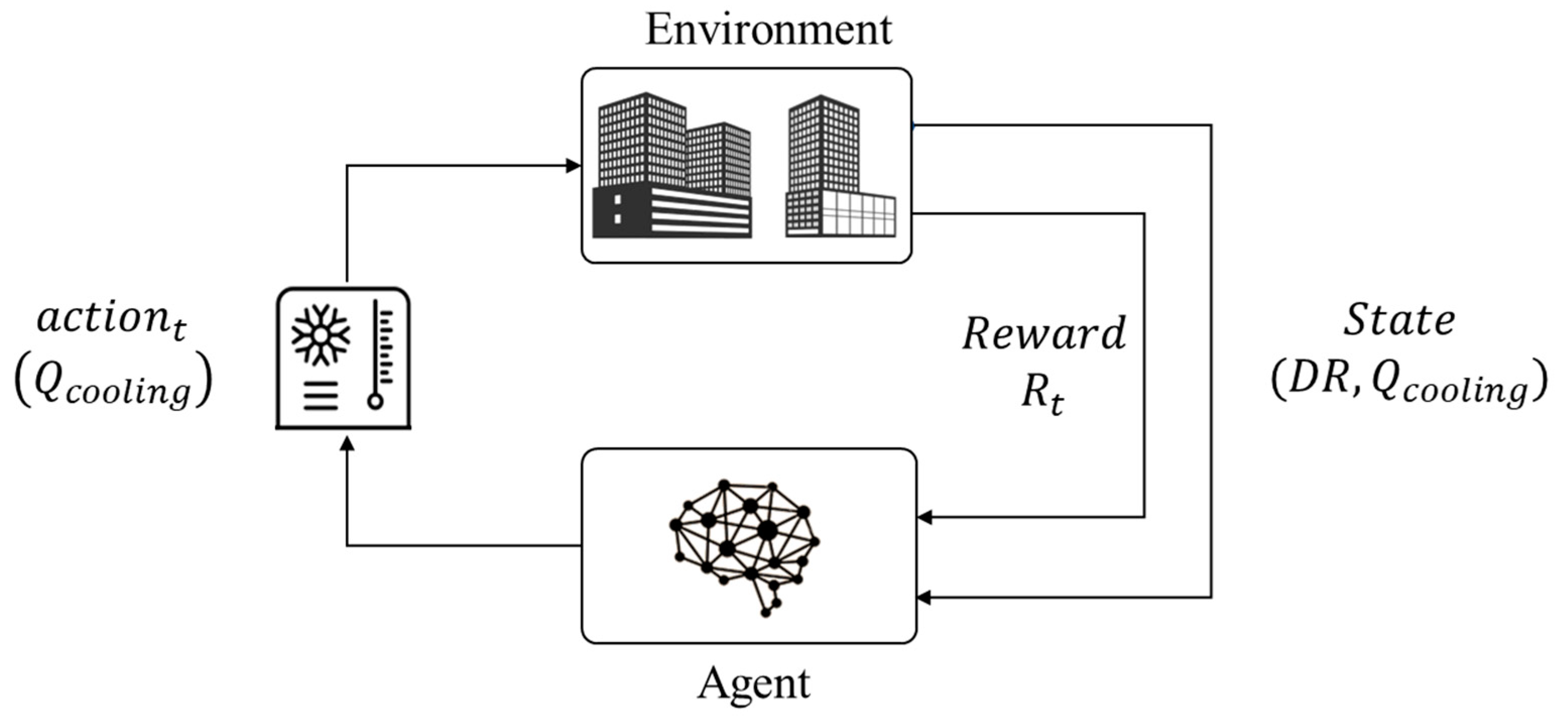
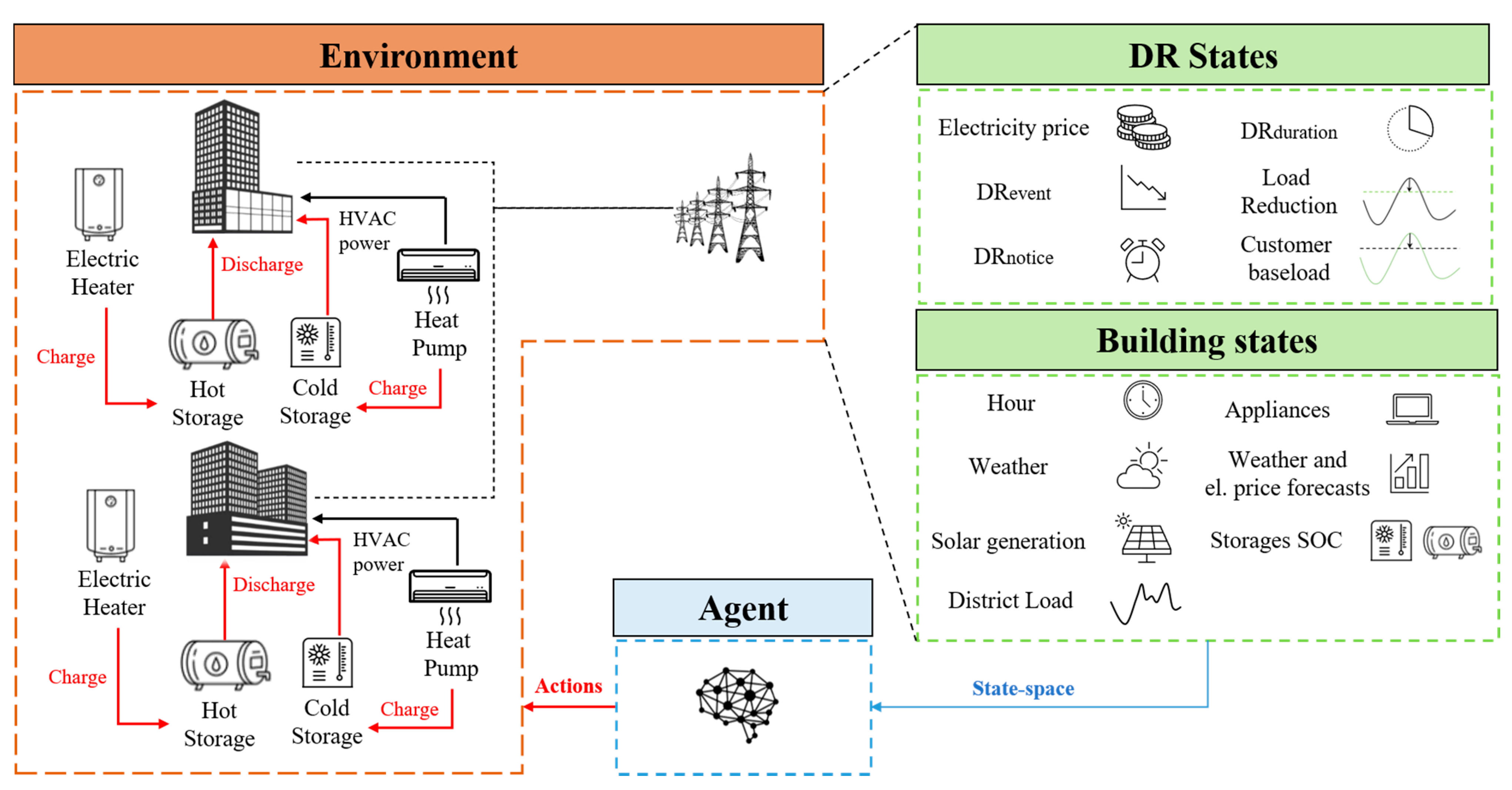
As a reference, Figure 2 shows a RL-based framework applied to a control problem concerning a building energy system. In Figure 2, the controller (agent) is supposed to be connected to a heat pump and a chilled water storage with the aim to satisfy the cooling energy demand of a building. The agent can take an action (e.g., charging or discharging the storage) when the environment is in a certain state (e.g., during a DR event) to optimize the building energy usage (i.e., parameter included in the reward function).

The most widely applied approach among RL algorithms, due to its simplicity, is the Q-Learning [59]. Q-Learning maps the relationships between states and action pairs exploiting a tabular approach [60] storing Q-values and selecting the set of optimal actions according to those values. The control agent gradually updates Q-values through the Bellman equation [61]:

$$Q\left(s,a\right) \leftarrow Q\left(s,a\right)+\lambda \left[r_t+\gamma {\max }_{a^{\prime }}Q\left(s^{\prime },a^{\prime }\right)-Q\left(s,a\right)\right]$$

(3)

where λ (0,1) is the learning rate, which determines how rapidly new knowledge overrides old knowledge. When λ = 0, no learning happens, while for λ set equal 1, new knowledge completely overrides what was previously learned by the control agent. Despite the effectiveness, due to large state and action spaces that need to be stored, the tabular representation is inadequate in real-world implementations. In this paper, the Soft Actor–Critic (SAC) algorithm, an actor–critic method, was employed. SAC is an off-policy algorithm based on the maximum entropy deep reinforcement learning framework, introduced by Haarnoja et al. [62]. Unlike Q-learning, SAC is capable of handling continuous action spaces, extending its applicability to various control problems. A detailed description of the SAC algorithm is provided in the following subsection.

Soft Actor–Critic

Soft Actor–Critic exploits the actor–critic architecture, approximating the state-value function and the action-value function using two different deep neural networks. In particular, the Actor maps the current state based on the action it estimates to be optimal, while the Critic evaluates the action by calculating the value function. Furthermore, the off-policy formulation allows reusing previously collected data stored in a replay buffer (D), increasing data efficiency.

SAC learns three different functions: (i) the actor (mapped through the policy function with parameters $\varphi$), (ii) the critic (mapped with the soft Q-function with parameters $\theta$), and (iii) the value function V, defined as:

$$\begin{gathered} V\left(s_t\right)={\mathbb{E}}_{a_t~\pi }\left[Q\left(s_t, a_t\right)-\alpha \log \pi \left(a_t|s_t\right)\right] \\ ={\mathbb{E}}_{a_t~\pi }\left[Q\left(s_t, a_t\right)\right]+\alpha {\mathbb{E}}_{a_t~\pi }\left[\log \pi \left(a_t|s_t\right)\right] \\ ={\mathbb{E}}_{a_t~\pi }\left[Q\left(s_t, a_t\right)\right]+\alpha H \end{gathered}$$

(4)

The main feature of SAC is the entropy regularisation: this algorithm is based on the maximum entropy reinforcement learning framework, in which the objective is to maximize both expected reward and entropy [63] as follows:

$${\pi }^{\ast }=\arg \underset{{\pi }_{\varphi }}{\max }{\displaystyle \sum }_{t=0}^T{\mathbb{E}}_{\left(s_t, a_t\right)~{\rho }_{\pi }} \left[r\left(s_t, a_t\right)+\alpha H\left({\pi }_{\varphi }\left(·|s_t\right)\right)\right]$$

(5)

where ${\left(s_t, a_t\right)}_{\sim {\rho }_{\pi } }$ is a state–action pair sampled from the agent’s policy, $r\left(s_t, a_t\right)$ is the reward for a given state–action pair, and H is the Shannon entropy term, which expresses the attitude of the agent in taking random actions.

SAC performances are influenced by the temperature parameter α, which determines the importance of the entropy term over the reward. Furthermore, to reduce the effort required for tuning this hyperparameter, the paper exploits a recent version of the SAC that employs alpha automatic optimization [62].

3. Case Study and Control Problem

The case study focused on the energy management optimization of a cluster of buildings considering the possibility to integrate DR signals in the control strategy. The considered cluster included four commercial buildings: a small office, a restaurant, a stand-alone retail, and a strip mall retail. The four buildings analyzed belonged to commercial reference buildings developed by U.S. Department of Energy (DOE). Each building was equipped with a heat pump used to charge a cold storage and to satisfy the heating and cooling energy demand of the building. Moreover, buildings used electric heaters and hot storages to meet the DHW demand. The Heat Pump Size ($H{P}_{size}$) was defined considering the maximum hourly cooling demand ($E_{cooling,max}$) and a Safety Factor (SF) equal to 2.5 for taking into account the reduced capacity during low external temperatures periods [64]:

$$H{P}_{size}=E_{cooling,max}\ast SF \left[\mathrm{kW}\right]$$

(6)

The storages capacity ($C_{cooling}$ for cooling and $C_{DHW}$ for DHW storages) was designed according to the maximum hourly energy demand for cooling and DHW ($E_{DHW,max})$, considering a Capacity Factor (CF) equal to 3 [65]:

$$C_{cooling}=E_{cooling,max}\ast CF \left[\mathrm{kWh}\right]$$

(7)

$$C_{DHW}=E_{DHW,max}\ast CF \left[\mathrm{kWh}\right]$$

(8)

Table 1. Building and energy system properties.

Building Number	Type	Surface [m2]	Volume [m3]	Heat Pump Capacity [kW]	Cold Storage Capacity [kWh]	Hot Storage Capacity [kWh]	PV Capacity [kW]
1	Small Office	5000	13,700	748	898	16	50
2	Restaurant	230	710	197	158	33	0
3	Stand-alone Retail	2300	14,000	533	639	0	0
4	Strip Mall Retail	2100	10,800	660	792	0	40

reports for each building the geometrical features and the details about the energy systems, together with Photovoltaic (PV) system size.

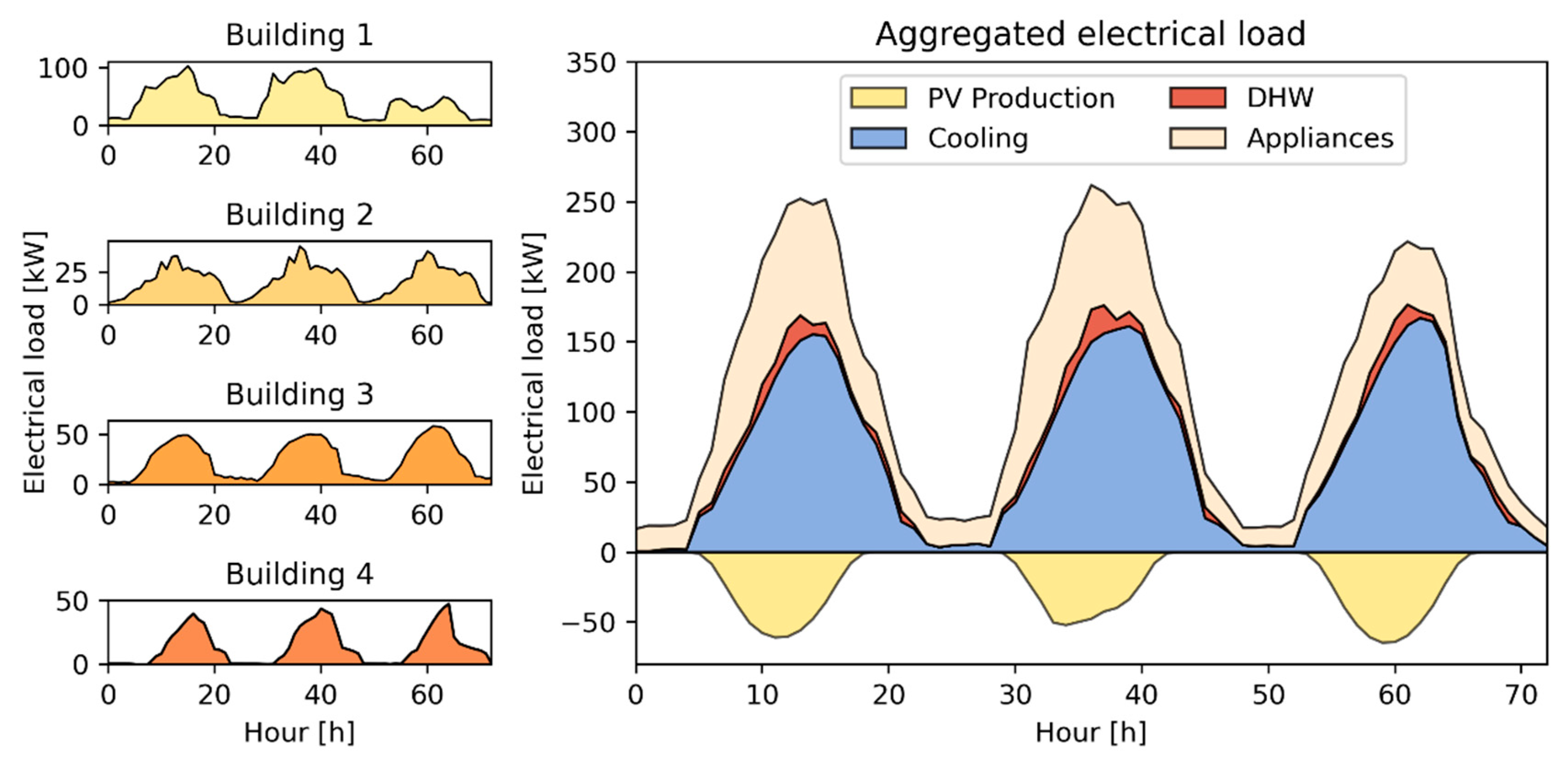
Figure 3 shows the electric load profile of each building and for the entire district for the first 3 days of simulations during the cooling season. In particular, the left side of Figure 3 highlights the heterogeneity of both shape and intensity of the electric consumption. The right side shows the disaggregation of the total district load into cooling, DHW, non-shiftable appliances, and PV production. The control problem was tested over a three-month period during summer (from 1 June to 31 August) when the cooling energy demand was the main driver of the building cluster consumption.

3.1. Description of the Control Problem

In this paper, the RBCs and DRL-based control strategies were implemented and tested in CityLearn [66], a simulation environment based on OpenAI Gym [67]. The environment has the aim to ease the training and evaluation of the RL controller in DR scenarios considering a heterogeneous cluster of buildings. CityLearn received input pre-simulated building hourly data and allowed the control of the charging and discharging of the thermal energy storage devices installed in the buildings. The heating energy was supplied by electric heaters while cooling energy was supplied by air-to-water heat pumps. Furthermore, some buildings were equipped with a PV system to produce on-site energy.

The controllers were designed to manage the charging and discharging of cooling and DHW storages for the district of buildings, with the aim to minimize electricity costs and reduce electrical load as requested during the incentive-based DR events considered. The electricity costs and the DR programs tariffs were the main drivers of the control problem. In particular, an electricity price (c_El) that varied from c_El,off-peak = 0.01891 €/kWh during off-peak hours (9 p.m.–12 a.m.) to c_El,on-peak = 0.05491 €/kWh during on-peak hours (12 a.m.–9 p.m.) was considered. Moreover, a cost related to the monthly peak load ($C_{Peak}$) was considered and defined below:

$$C_{Peak}=c_{Peak}\ast P_{Monthly, Peak} [€]$$

(9)

where C_Peak [€/kW] is the tariff related to the monthly peak load PMonthly,Peak [kW], evaluated as the maximum aggregated electrical load per each month related to the entire cluster of buildings.

The DR income (I_DR) was set according to the tariffs defined by an Italian electricity provider. In detail, the overall DR remuneration was defined in Equation (10):

$$I_{DR}=I_{Fixed}+I_{Variable} [€]$$

(10)

I_Fixed corresponds to the fixed user profit due to the participation in the DR program. This remuneration is defined according to Equation (11):

$$I_{Fixed}=I_{Power}\ast LR [€]$$

(11)

where I_Power (€/kW/year) is the tariff related to the Load Reduction (LR) [kW] requested during DR event and contracted between users and provider.

The variable term of DR income (I_Variable) is defined according to Equation (12) and takes into account the reduction in energy demand from the grid as requested by the DR program:

$$I_{Variable}={\displaystyle \sum }_{i=1}^N{I}_{Energy}\ast \min \left\{LR,CB{L}_i-P_{i,District}\right\}\ast D{R}_{duration}$$

(12)

where I_Energy (€/kWh) is the tariff related to the energy reduction for DR. I_Variable exploits the concept of Customer Baseload (CBL), defined as the sum of cooling, DHW, and appliances power minus the PV production, without considering the effect on the electrical load of the storage operation. In particular, I_Variable was evaluated as the difference between the customer baseload and the aggregated load (P_District) during the DR period, multiplied by the duration of the DR (DR_duration). Moreover, the incentive was limited up to the contracted power (LR), and a further reduction beyond LR would not be remunerated. IPower equal to 30 €/kW/year, I_Energy = 0.25 €/kWh, and LR = 35 kW were assumed to simulate a realistic scenario. The DR call (DR_event) was assumed to be stochastic, with a random duration between 2 and 4 h during the period 2 p.m.–8 p.m. (DR_duration), considering the notification of the customer 1 h before the event start (DR_notice) and limiting its occurrence at no more than one DR event per day, according to realistic strategies adopted by an electricity provider.

4. Methodology

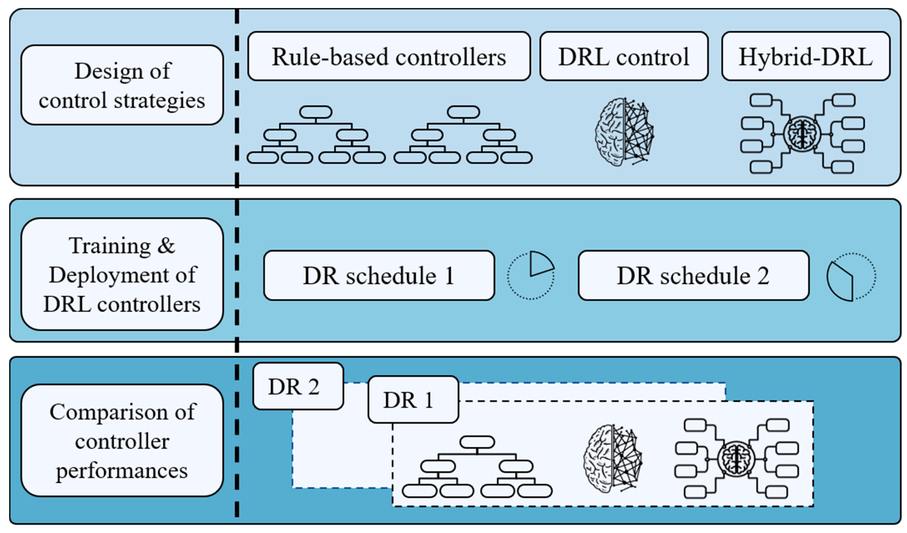
This section reports the methodological framework adopted in the present paper (Figure 4). First, two RBC and two DRL-based controllers were selected in order to assess the advantages related to advanced control strategies. Then, DRL-based controllers were trained and deployed to check the quality of control policies. Lastly, control performances were analyzed, taking into consideration both pros and cons of each proposed strategy. The main stages of the methodological process are below described.

Design of control strategies: the first stage of the process is aimed at defining the different approaches adopted in this paper, starting from state-of-the-art RBC controllers up to advanced DRL and hybrid DRL strategies.

• Design of baseline rule-based controllers: two rule-based control strategies were defined in the study. The first one (RBC-1) optimized cluster electrical load without considering the participation of buildings in DR events during the entire simulation period. Such RBC controller was used as a reference baseline against controllers which consider DR signals in order to explicitly assess the benefits for the users and for the grid when such feature of the controller is enabled.
  On the other hand, the second RBC controller (RBC-2) was designed with the ability to satisfy DR requirements. Different from RBC-1, this one represented a credible benchmark for more advanced controllers based on DRL and hybrid-DRL approach that were considered in this study for addressing the control problem.
• Design of deep reinforcement learning controller: the formulation of the DRL controller started from the definition of the action-space, which included all the possible control actions that could be taken by the agent. Then, the state-space was defined, including a set of variables related to the controlled environment, which led the agent to learn the optimal control policy. Lastly, the reward function was designed with the aim to address the considered multi-objective control problem robustly. Such controller was then compared against the RBC strategies in order to assess its pros and cons and better drive the design of a hybrid control logic in which DRL and RBC were coupled.
• Design of hybrid deep reinforcement learning controller: the controller was designed to exploit the predictive nature of the DRL, while maintaining the deterministic nature of the RBC, with the aim to maximize economic benefits for the users by minimizing the violation of DR constraints during incentive-based events. This controller used the same state–action space of the DRL controller with a different reward function that did not take into account the fulfilment of DR requirements. In particular, during the simulation of DR events, the hybrid control logic used actions provided by the RBC, overwriting DRL control signal, always ensuring DR requirements satisfaction. On the other hand, during the remaining part of the day, the controller exploited the predictive nature of the DRL algorithm to optimize storage operation, reducing energy costs.

Training and deployment of DRL-based controllers: after the design of the control strategies, the two DRL-based controllers were trained offline, using the same training episode (i.e., a time period representative of the specific control problem) multiple times, continuously improving the agent control policy. Then, the DRL and hybrid-DRL agents were first tested with the same schedule of DR events used for training, with the aim to analyze the effectiveness of the learned control policy specifically. Then, to evaluate their robustness and adaptability capabilities, the control agents were deployed considering a schedule of DR events completely different from training.

Comparison of controller performances: lastly, the four controllers (i.e., RBC-1, RBC-2, DRL, and Hybrid-DRL) were compared to identify the strengths and weaknesses of each one explicitly. The DRL-based approaches were compared with RBCs, due to their wide-spread real-world implementation. Therefore, RBCs were used as a benchmark also according to the approach adopted in [56,64]. In this work, first, a cost disaggregation was provided for each control strategy, identifying the advantages to join incentive-based DR programs and highlighting the role of storage control for managing thermal-sensitive electrical loads in buildings. Then, the analysis focused on the impact the participation in DR events has on the grid, also identifying possible risk of peak rebound (i.e., the occurrence of a peak condition after the demand response event).

5. Implementation

This section describes how the four controllers were designed. In addition to the two rule-based controllers, used as baselines, a detailed description of state-space, action-space, and reward functions of DRL and hybrid-DRL agents is provided in the following.

5.1. Baseline Rule-Based Controllers

Two rule-based controllers were used to compare the effectiveness of the DRL and hybrid-DRL controller. In particular, the first rule-based controller (RBC-1) was designed to reduce energy costs of each building, exploiting the variability of electricity tariffs during the day, and did not consider any participation in incentive-based DR events.

For RBC-1, both chilled water and DHW storages were charged during the night period and heat pumps could operate more efficiently in cooling mode when the electricity price was lower, thanks to lower temperatures. In addition, both charging and discharging actions were uniform throughout the day to reduce peak consumption and flatten the electrical load profile. Equation (13) better clarifies the charging/discharging strategy for the RBC-1.

$$a_{RBC-1}=\{\begin{array}{c}-\raisebox{1ex}{$1$}\!\left/ \!\raisebox{-1ex}{$\Delta t$}\right. \mathrm{if} 8 \mathrm{a}.\mathrm{m}.\le t\le 7 \mathrm{p}.\mathrm{m}.\\ 0.1 \mathrm{else}\end{array}$$

(13)

where a_RBC-1 represents the action taken by the RBC-1 agent and Δt the number of hours (i.e., 12 h) for which the electricity cost is equal to c_El,on-peak.

Conversely, the second rule-based controller (RBC-2) was designed to exploit electricity tariffs and participate in incentive-based DR programs. In more detail, in the absence of DR events, RBC-2 performed the same actions as RBC-1. On the other hand, in the presence of a DR event, the RBC-2 modified its actions according to the notified DR duration and the State of Charge of the thermal storages (SOC), to meet contracted load reduction without influencing user comfort. Specifically, the controller pre-charged storages if their SOC was not sufficient to satisfy the required load reduction, while it continued to discharge if the state of charge could meet grid request. The selected control actions and associated constraints are indicated as follows.

• If 8 a.m. ≤ t ≤ 7 p.m.:

$$a_{RBC-2}=\{\begin{array}{c}-\raisebox{1ex}{$1$}\!\left/ \!\raisebox{-1ex}{$\Delta t$}\right. if D{R}_{notice}=1 and D{R}_{event}=0 and SOC>\raisebox{1ex}{$1$}\!\left/ \!\raisebox{-1ex}{$\Delta t$}\right.\ast \left(1+D{R}_{duration}\right)\\ \raisebox{1ex}{$1$}\!\left/ \!\raisebox{-1ex}{$\Delta t$}\right.\ast D{R}_{duration}-SOC if D{R}_{notice}=1 and D{R}_{event}=0 and SOC\le \raisebox{1ex}{$1$}\!\left/ \!\raisebox{-1ex}{$\Delta t$}\right.\ast \left(1+D{R}_{duration}\right)\\ -\raisebox{1ex}{$1$}\!\left/ \!\raisebox{-1ex}{$\Delta t$}\right. if not D{R}_{notice}=1 and D{R}_{event}=0 \end{array}$$

(14)

where a_RBC-2 represents the action taken by the RBC-2 agent, Δt is the same as the case of Equation (13), DR_notice is the notification received by the agent 1 h before the start of the DR event (DR_event), DR_duration is the duration of the DR event, and SOC is the state of charge of the considered storage.

• If 1 a.m. ≤ t < 7 a.m. and 8 p.m. ≤ t ≤ 12 p.m., the action selected by RBC-2 (a_RBC-2) corresponded to the one selected by RBC-1 under the same constraints.

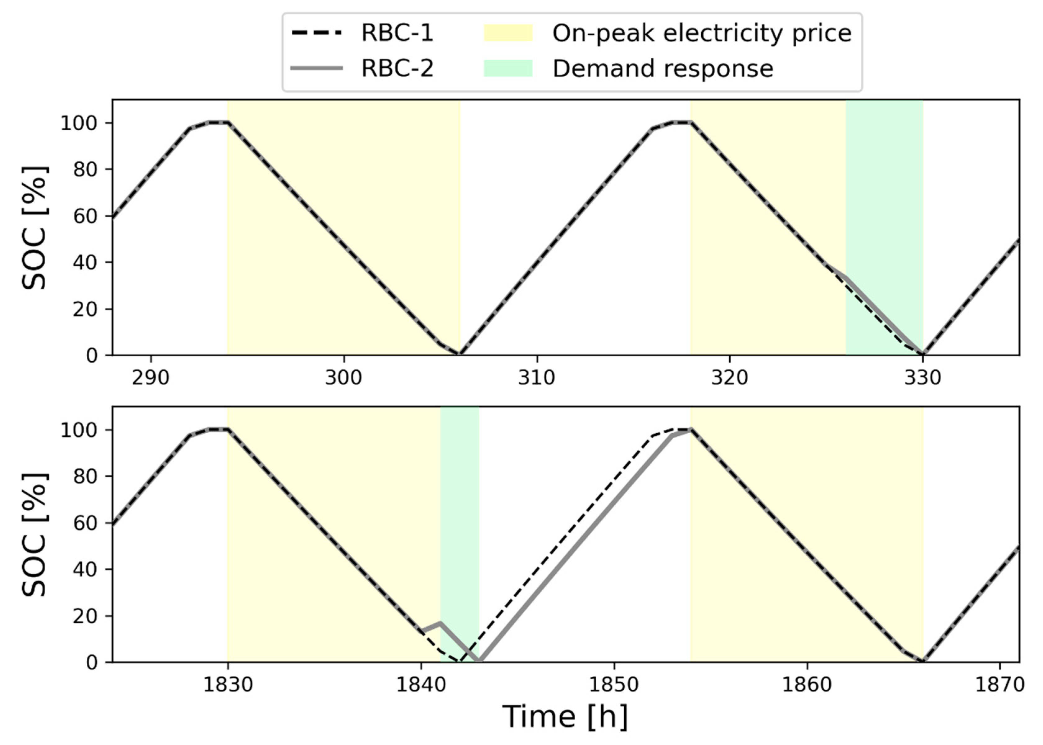
Figure 5 shows the behavior of the RBC agents for the cooling storage of a building in the considered cluster: the grey line represents the RBC-2 control policy, while the black dashed line pertains to the RBC-1 actions. The top part of the figure highlights the behavior of the two controllers in the absence and in the presence of DR events when in the latter case, a limited discharge rate reduction was performed by RBC-2 to avoid the full discharge of the storage before the end of the DR event. The bottom part of the figure refers to a different period and highlights the importance of the pre-charging strategy when the DR event takes place during the last on-peak hours, together with the effect on the subsequent charging process.

5.2. Design of DRL and Hybrid-DRL Controllers

This section is focused on the design of DRL and hybrid-DRL controllers for optimizing the energy consumption of the buildings in the considered district. The section includes the description of the action-space, state-space, and reward function. The controllers share the same action-space and state-space while the reward functions were differently conceived.

5.2.1. Design of the Action-Space

In this study, each of the four buildings in the district was equipped with a thermal cold storage and a heat pump to meet the cooling energy demand. In addition, buildings 1 and 2 (see

Table 2. State-space variables.

Variable	Unit
Weather
Outdoor Air Temperature	[°C]
Outdoor Air Temperature Forecast (1 and 2 h ahead)	[°C]
Direct Solar Radiation	[W/m2]
Direct Solar radiation Forecast (1 and 2 h ahead)	[W/m2]
Diffuse Solar Radiation	[W/m2]
Demand Response
DRevent	[-]
DRnotice	[-]
DRduration	[h]
Load reduction (LR)	[kW]
District
Electrical load (PDistrict)	[kW]
Customer baseload (CBL)	[kW]
Electricity Price Forecast (1 and 2 h ahead)	[€/kWh]
Hour of day	[h]
Day of the week	[-]
Month	[-]
Building
Non-shiftable load	[kW]
Solar generation	[kW]
Chilled water Storage SOC	[-]
DHW storage SOC	[-]

) met the DHW demand using heat storages supplied by an electric heater. Therefore, at each control time step (set equal to 1 h), the DRL agent provided six control actions related to the charge/discharge of the storages (i.e., four chilled water and two DHW storages). In detail, the DRL controller selected an action between [−1, 1], where 1 indicates a complete charge of the considered storage, and −1, its complete discharge. However, to represent a more realistic charging and discharging process, the action space was constrained between [−0.33, 0.33], considering that a complete charge or discharge of the storage lasts three hours, as in [65]. Moreover, CityLearn ensured that the heating and cooling energy demand of the building were always satisfied, overriding the actions of DRL-based controllers to satisfy such constraints of thermal energy demand [68].

5.2.2. Design of the State-Space

The state-space represents the set of variables seen from the control agent. A proper definition of these variables is crucial to help the controller in learning the optimal policy. The variables included in the state-space are reported in Table 2.

The variables were classified into weather, demand response, district, and building states. Weather variables, such as Outdoor Air Temperature and Direct Solar Radiation, were included to account for their influence on the cooling load. Moreover, their predictions with a time horizon of 1 and 2 h were used to enable the predictive capabilities of the controllers.

Through a boolean variable, the agent was informed of the occurrence of a DR event in the current time step (DR_event) and 1 h before (DR_notice). Moreover, DR states included information on the requested electrical load reduction (LR) and the elapsing time before the end of the DR event (DR_duration). Variables that were in common between all buildings in the cluster were included in district states, such as hour of day, day of the week, month, electricity price, and forecast of the electricity price with a time horizon of 1 and 2 h ahead. Furthermore, district variables also included the hourly net electricity demand (P_District) and the total pre-computed district demand, used as customer baseload (CBL).

The remaining states were categorized as building variables, such as the appliances’ electrical load (non-shiftable load), the photovoltaic electricity production (Solar generation), the state-of-charge of cooling and DHW storages (Chilled water storage SOC and DHW storage SOC).

Figure 6 shows a graphical representation of state and action spaces. The control agent received information on buildings, climatic conditions, and DR states for managing the charging/discharging of the thermal storages to optimize the energy usage at the district level, also considering the grid requirements.

5.3. Design of the Reward Functions

The reward function has to be representative of the defined control problem and assesses the effectiveness of the control policy. In this work, two separate reward functions were defined for the DRL and hybrid-DRL controllers, while the hyperparameters used for the controller design are reported in Appendix A.

5.3.1. Reward Function for DRL Controller

For the DRL controller, the reward was formulated as a linear combination of two different contributions, a DR-related term (R_DR) and a power-related term (R_P).

These terms were combined employing two weights (w_DR and w_P, respectively) that balance their relative importance. The general formulation of the reward is as follows:

$$R_{DRL}=\{\begin{array}{c}{w}_{DR}\ast R_{DR} \mathrm{if} D{R}_{event}=1\\ w_P\ast R_P \mathrm{if} D{R}_{event}=0\end{array}$$

(15)

The DR related term guaranteed the DRL control agent to endorse the network requests during the demand response event. The DR term was formulated according to Equation (16).

$$R_{DR}=\{\begin{array}{c}D{R}_{pen} \mathrm{if} P_{District}\ge CBL-LR\\ D{R}_{prize} \mathrm{if} P_{District}<CBL-LR\end{array}$$

(16)

Due to this formulation, the agent received a penalty DR_pen if the district load (P_District) during the DR period was higher than the electrical load threshold, defined as the difference between the customer baseload and the contracted load reduction, otherwise, it received a prize DR_prize. On the other hand, the power term of the reward R_P had different expressions depending on electricity cost c_El, as defined in the following:

$$R_P=\{\begin{array}{c}{R}_{P,off-peak} \mathrm{if} {\mathrm{c}}_{El}=c_{El,off-peak}\\ R_{P,on-peak} \mathrm{if} {\mathrm{c}}_{El}=c_{El,on-peak}\end{array}$$

(17)

Furthermore, the two parts of the power-related terms (R_P,off-peak and R_P,on-peak) depend on the electrical load of the building district P_District, as expressed in Equations (18) and (19).

$$R_{P, off-peak}=\{\begin{array}{c}{p}_{P_1} if t{h}_{1, off-peak}\le P_{District}\le t{h}_{2, off-peak}\\ p_{P_2} else\end{array}$$

(18)

$$R_{P, on-peak}=\{\begin{array}{c}{p}_{P_1} \mathrm{if} t{h}_{1,\mathrm{on}-\mathrm{peak}}\le P_{District}\le t{h}_{2,\mathrm{on}-\mathrm{peak}} \\ P_{District}-t{h}_{1,on-peak} \mathrm{if} P_{District}\le t{h}_{1,\mathrm{on}-\mathrm{peak}}\\ \left(t{h}_{2,on-peak}-P_{District}\right)\ast K_P \mathrm{if} P_{District}\ge t{h}_{2,\mathrm{on}-\mathrm{peak}}\end{array}$$

(19)

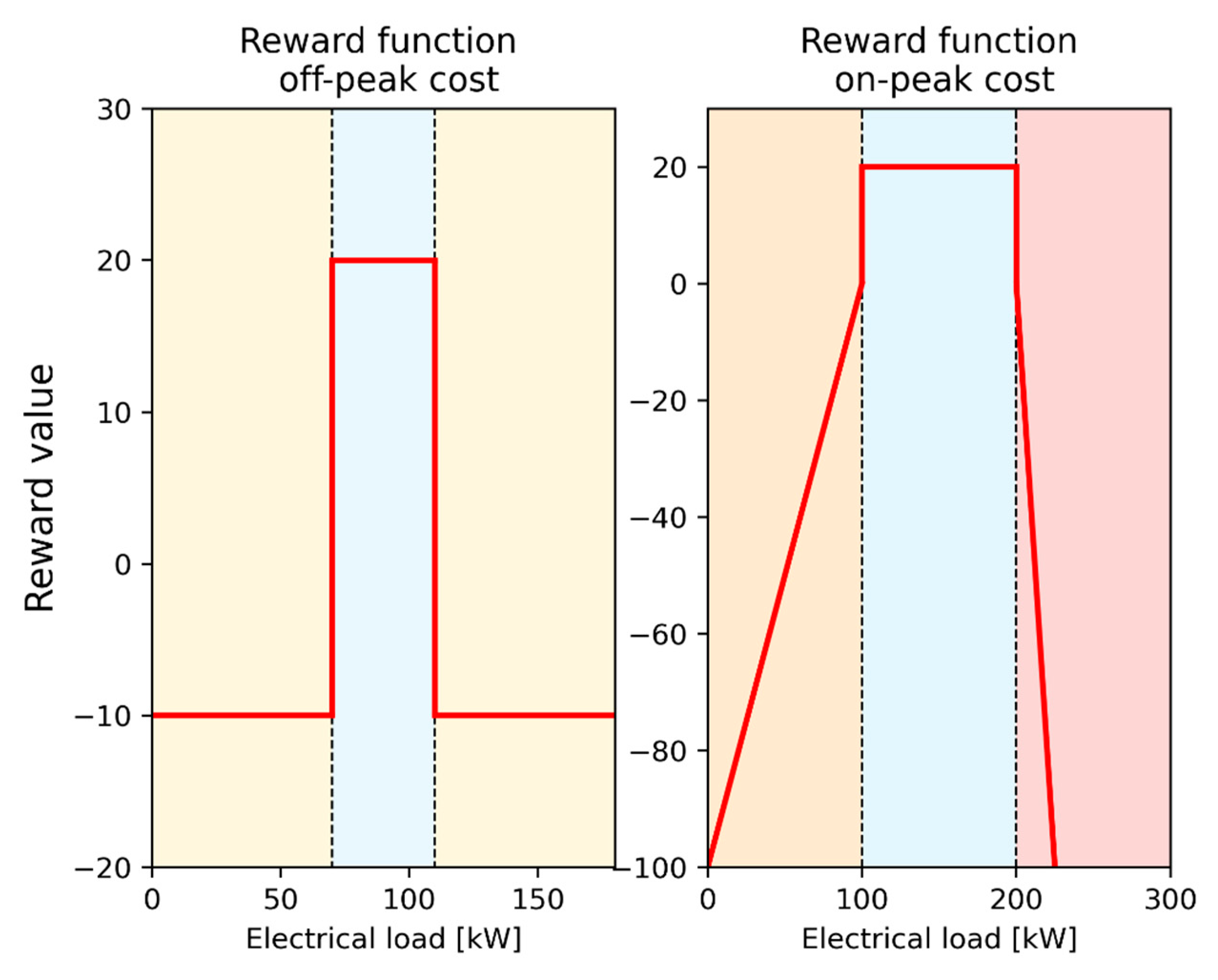
The formulation of the power term, shown in Figure 7, was conceived to flatten the load profile. A number of thresholds were selected based on the load duration curve of the cluster of buildings, therefore being case-specific to solve this problem.

In particular, during off-peak periods, two thresholds were used to incentivize consumption between the 40th percentile (th1,off-peak) and the 50th percentile (th2,off-peak), rewarding (with a fixed prize term p_P1) or penalizing (with a fixed penalty term p_P2) the controller. This reward formulation penalizes low values of electrical load, associated with storage discharge or no usage, and high values of electrical load, which represent a sudden charging of the storages. On the other hand, an electrical load between the two thresholds was incentivized, denoting a homogeneous storage charge over time.

Conversely, during on-peak periods, consumption was incentivized between the 45th percentile (th1,on-peak) and the 80th percentile (th2,on-peak), associating this interval with an optimal storage use. Similar to the off-peak periods, a load lower than th1,on-peak was penalized, being associated with a sudden discharge, while a penalty multiplier (K_P) was introduced for load higher than th2,on-peak to prevent the occurrence of peaks. The values chosen for all DRL reward terms are reported in

Table 3. Values assumed for DRL reward function features.

Variable	Value
$w_{\mathrm{DR}}$	0.035
$w_{\mathrm{P}}$	0.1
$D{R}_{pen}$	−45,000
$D{R}_{prize}$	10,000
$p_{{\mathrm{P}}_1}$	20
$p_{{\mathrm{P}}_2}$	−10
$t{h}_{1,\mathrm{off}-\mathrm{peak}}$	70
$t{h}_{2,\mathrm{off}-\mathrm{peak}}$	110
$t{h}_{1,\mathrm{on}-\mathrm{peak}}$	100
$t{h}_{2,\mathrm{on}-\mathrm{peak}}$	200
$K_{\mathrm{p}}$	30

.

5.3.2. Reward Function for the Hybrid-DRL Controller

The hybrid-DRL controller (DRL-RBC) exploited the same structure of the deep reinforcement learning controller, while during demand response events, it used the RBC-2 control strategy to address load reduction requests. For the hybrid controller, the reward function only consisted of a power-related term that aimed to flatten the load profile, expressed in the following way:

$$R_{DRL-RBC}=\{\begin{array}{c}-w_1\ast \left(P_{District}-t{h}_{Peak}\right) if P_{District}\ge t{h}_{Peak}\\ p_1 else\end{array}$$

(20)

The reward highly penalized a load greater than th_Peak, chosen as the 95th percentile of the load duration curve. This formulation allowed the controller to learn how to flatten the load profile while fulfilling grid requirements. The values chosen for the hybrid-DRL reward terms are indicated in

Table 4. Values assumed for hybrid-DRL reward function features.

Variable	Value
$w_1$	100
$p_1$	10
$t{h}_{\mathrm{Peak}}$	300

.

6. Results

The section describes the results of the implemented framework. First, performances during training periods of the developed DRL and hybrid-DRL controllers were compared with the RBC-2, to explore how the different controllers handled the occurrence of DR events. In detail, the load profile of all buildings in the district, comparing the storage charging/discharging process of the controllers and the associated overall costs was analyzed. Moreover, RBC-1 was compared with other controllers to assess the user advantages when participating in DR programs.

Afterward, to test the robustness of the controllers, the results obtained using a different deployment schedule of DR events are discussed.

6.1. Training Results

This subsection presents the results of the developed controllers deployed on the same schedule used for the training phase.

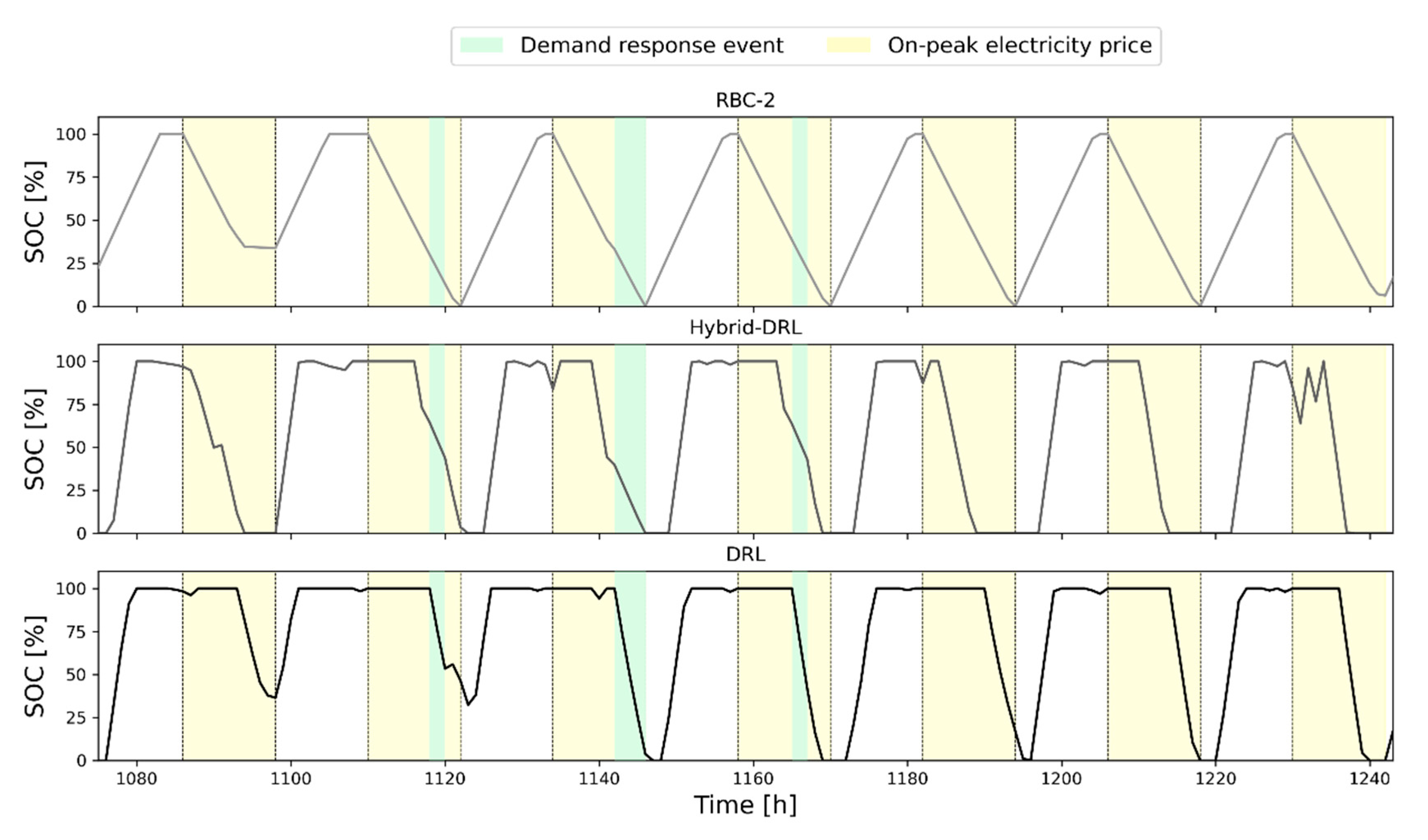
Figure 8 reports the comparison between RBC-2 (on the top), hybrid-DRL (in the middle), and DRL (on the bottom) controllers during a typical week of the analyzed period, considering the chilled water storage charging/discharging process of building 3. As previously explained, RBC-2 agent charged the storage during the off-peak periods in order to discharge it during peak hours. In addition, the amount of energy discharged was influenced by the DR program requirements (green zone), as shown in the upper part of Figure 8 by the slope variation during the third day of the considered week. The DRL and hybrid-DRL controllers exhibited a storage charging process similar to the RBC-2, while the discharging one was differently managed. Although the cost of electricity was higher during the on-peak hours, the DRL agent chose to maintain a high SOC of the storage to meet the energy demand reduction by discharging the storage during the DR periods. On the other hand, the hybrid-DRL controller discharged the storage, taking into account the higher cost of energy as well as the necessity to reduce the energy demand, achieving an energy saving of 7%. Therefore, the discharging process started approximately in the middle of the on-peak period, ensuring that the storage had sufficient charge to satisfy the potential occurrence of a demand response event.

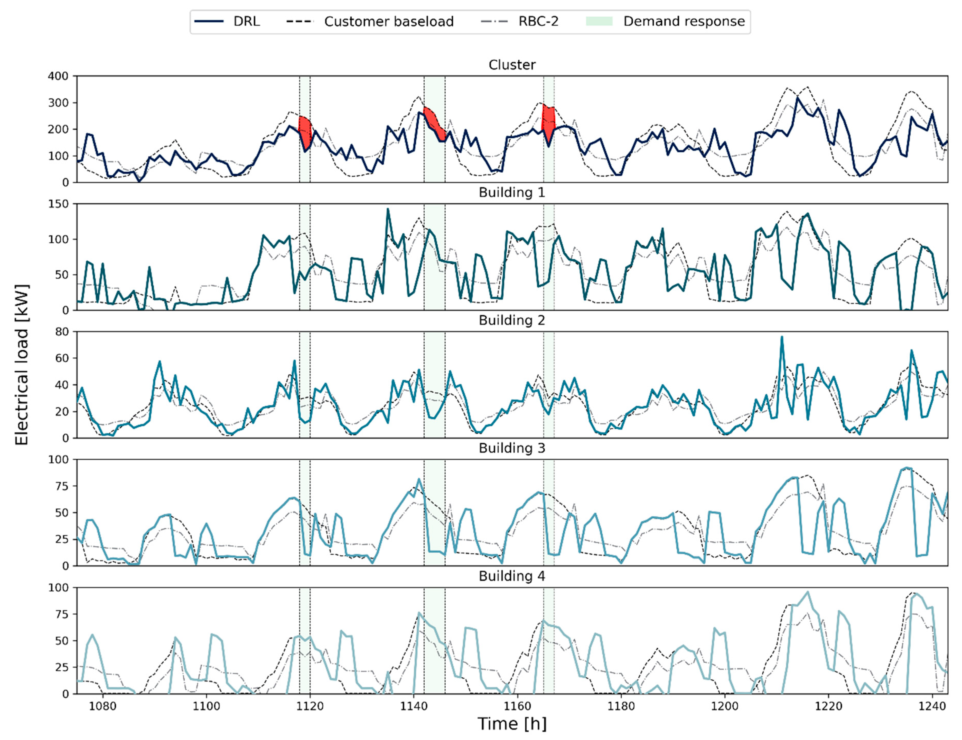
Figure 9 shows the comparison between the different control strategies for the cluster (top part of the figure) and each building. In particular, the figure shows the effects of two control strategies (RBC-2 and DRL) on the load profiles, considering as reference the customer baseload. As shown in the upper part, the aggregated load profile resulting from the DRL controller was more uniform than that resulting from RBC-2. Moreover, the DRL agent showed greater adaptability to DR programs, optimizing both cluster load profile, energy costs, and load reduction during DR events.

On the other hand, the analysis at a single building level showed that, during DR events, the centralized agent achieved load reduction by meeting the cooling and DHW demand of building 2 and building 3 through the discharge of thermal storages. This result highlighted the possibility to further reduce the load using the storages of building 1 and 4, representing an additional source of flexibility for the cluster. Lastly, it could be noticed that although single building profiles presented higher peaks than RBC-2, the aggregated load displayed a flatten profile.

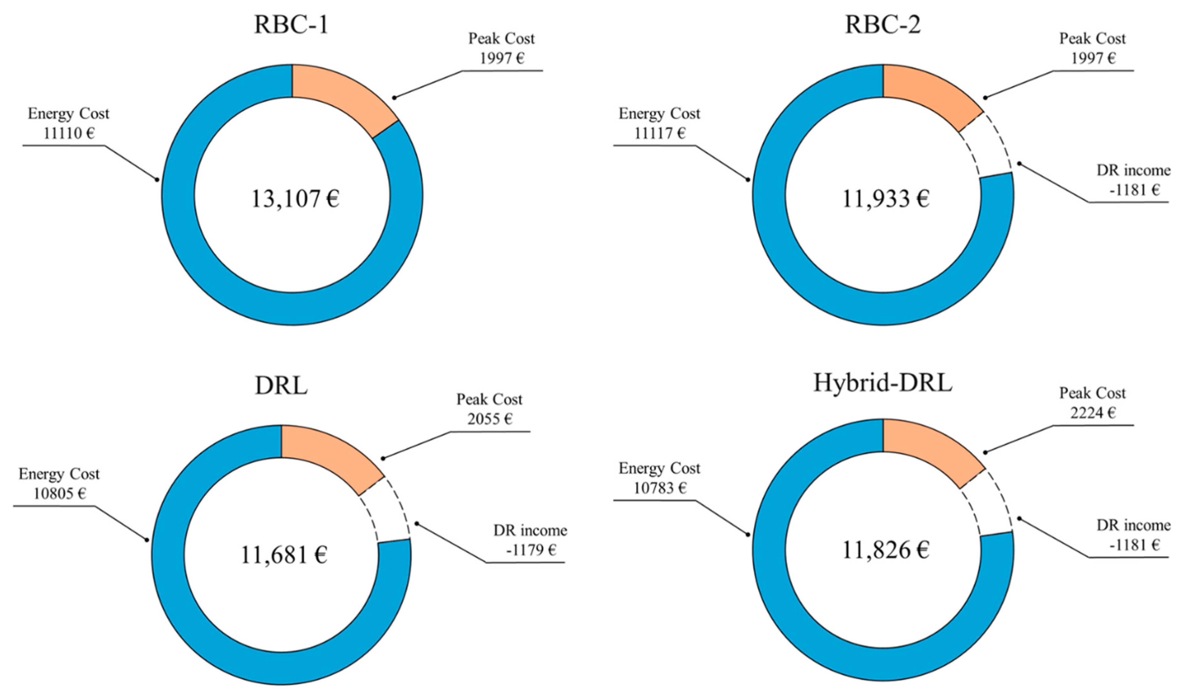
Lastly, Figure 10 reports a comparison of the cost disaggregation obtained for each controller, according to the definition of the total cost given in Section 3.1. Overall, the DRL controller was the most cost-effective due to optimal management that allowed the agent to minimize costs related to energy consumption, also meeting grid requirements. The DRL agent violated the DR program for 1 h out of a total of 105 due to a lack of storage charge, allowing the agent to remain within the DR program and earning 1179 €. The hybrid-DRL and the RBC-2 control policies led to higher costs, despite the absence of violations over the entire demand response period. The hybrid agent was able to exploit the variability of energy tariffs during the day and minimize the energy costs by leveraging the adaptive capabilities of reinforcement learning. Although the peak cost was 10% higher than the RBC-2, the total cost was lower. On the other hand, the RBC-1 agent was used to assess user benefits for participating in incentive-based DR programs. In particular, the comparison among the two RBC highlights how, despite the slight increase in energy costs, the participation in DR programs led to overall savings of around 9%.

6.2. Deployment Results

This subsection describes the results obtained by testing DRL and hybrid-DRL controllers on the same simulation period used for training but considering a different DR schedule to evaluate their adaptive capabilities. The new DR schedule consisted of 69 h, compared to 105 h, considered in the training phase. The performances of the developed controllers were compared with the RBC agents in

Table 5. Cost disaggregation: a comparison between the developed agents during the deployment phase.

Controller	Energy Cost [€]	Peak Cost [€]	DR Income [€]	Total Cost [€]
RBC-1	11,110	1997	0	13,107
RBC-2	11,114	1997	−866	12,245
DRL	10,864	2014	−851	12,027
Hybrid-DRL	10,685	2335	−866	12,154

.

Results showed that DRL controller again ensured the lowest cost, minimizing energy and peak costs. However, the profit associated with the participation in the demand response program was lower due to 3 h of violations, during which the controller did not guarantee load reduction. It must be noticed that in some cases, the violations might be unacceptable in the contracts defined with the grid operators, leading to the exclusion from the DR program.

On the other hand, the hybrid-DRL agent led to the highest peak cost due to a sudden charge of storages to satisfy DR events, whose effects were balanced by a reduction of 4% of the energy costs.

7. Discussion

The present paper aims to exploit deep reinforcement learning to optimally control thermal storages of four small commercial buildings under an incentive-based demand response program. The study focused on the comparison of different control strategies to investigate the advantages and limitations of each controller. In particular, the RBC-1 was introduced as a baseline to assess the benefits of demand response programs for the users considered in RBC-2 and DRL-based controllers.

On the other hand, RBC-2 was introduced to analyze and benchmark the effect of exploiting advanced control strategies coupled with demand response programs in multiple buildings, assessing the advantages of DRL controllers in reducing energy costs.

The paper proposed the implementation of automated demand response with particular attention to costs related to energy consumption, peak occurrence, and DR remuneration. This approach led to the identification of the advantages of a data-driven strategy with respect to a standard rule-based one.

Due to its adaptive nature, DRL exploited weather forecast conditions to maximize heat pump efficiency, reducing energy costs. Moreover, different from RBC or hybrid controllers, the DRL agent satisfied load reduction with a centralized approach, using only a part of the storages of the buildings to meet load reduction. Due to better exploitation of building flexibility, the centralized approach provided the opportunity to increase the contractualized power, which will further reduce costs. The main limitation of the DRL controller was related to the high effort necessary for the definition of the reward function. In particular, the DR event was highly stochastic, leading to a sparse reward that must be carefully managed. As a result, the design of the reward function was case-specific since it used several thresholds deriving from the load duration curve. This concept provided the motivation for the creation of the hybrid controller.

Conversely, the RBC-2 controller ensured the fulfillment of grid requirements during DR events at the expense of system efficiency by operating a uniform charge and discharge of storages.

Lastly, the hybrid controller experienced a slight cost reduction with respect to the RBC-2, highlighting the ability of the controller to optimize energy consumption while guaranteeing DR satisfaction.

Furthermore, the study also analyzed how the change in the DR schedule can influence control performances, studying the effect of such modification on energy costs and DR violations. Despite the effectiveness of the DRL controller to reduce energy costs, this paper highlighted some limitations related to its readiness in reacting to stochastic DR events that could lead to exclusion from the DR programs.

The paper showed that although a tailored RBC (i.e., RBC-2) was always able to meet grid requirements during incentive-based DR events, it was not able to exploit flexibility sources also improving energy efficiency. The DRL was able to optimize the performance of the heat pump during operation, efficiently exploiting climate conditions and variable energy tariffs for charging the thermal storages but with some violations of DR constraints. Such an outcome suggests that DRL is more suitable for time-based DR, in line with current literature.

On the other hand, the hybrid-DRL controller was designed to exploit the predictive nature of the RL while maintaining the deterministic nature of the RBC, with the aim to maximize economic benefits for the users and to minimize the violation of DR constraints during incentive-based events, representing a valuable alternative to state-of-the-art RBC controllers.

This approach seems to represent a promising trade-off between cost reduction, design simplicity, and the ability to meet grid requirements. In addition, these benefits can further increase with the amount of the energy flexibility bid in the flexibility market. However, the practical implementation of a DRL-based controller still remains more complex than an RBC but not far away from a feasible penetration in the real world. In this context, the increasing availability of building-related data can be exploited to effectively pre-train the RL agent and speed up the online learning process, while weather forecast, and grid information can be easily retrieved through specific services.

8. Conclusions and Future Works

The present work has shown the applicability of an adaptive control strategy based on deep reinforcement learning to thermal storage management under incentive-based DR programs. In particular, the study focused on different control paradigms, starting from two standard rule-based controllers, one of them (i.e., RBC-2) designed to fulfill the DR program, up to a more complex model-free DRL agent. Moreover, an additional hybrid solution, which exploits the ability of DRL to optimize energy usage and the deterministic actions of the RBC during the DR events, was proposed. The paper highlighted how participation in DR programs could be useful for the users, that even with a simple RBC, costs could be reduced by 9%. Moreover, these advantages could be enhanced using predictive controllers, such as DRL or hybrid-DRL. The deployment of the agents on unseen DR schedules during training confirmed the previous considerations on energy costs, highlighting the inability of the DRL controller to fully adapt to the stochastic behavior of DR. Therefore, the DR income for the DRL control agent was lower than the ones obtained for RBC-2 and hybrid-DRL agent since it violated the DR program for 4% of the hours. The hybrid-DRL agent, instead, mixed the benefits of the two approaches, using the rule-based controller to quickly react to grid necessities while exploiting the predictive nature to reduce energy costs by 4% with respect to RBC-2, thus representing a promising solution to further explore with different configurations of energy systems and size of the cluster of buildings, also considering practical applications.

Future works will be focused on the following aspects:

• The implementation of a decentralized approach for the DRL controllers, in which all agents can cooperate. This approach could provide numerous opportunities. In particular, the reward function can be designed differently for each building to decide the relative importance among the objectives, such as flattening the load profile or ensuring compliance with the DR program.
• Introducing dynamic electricity price tariffs and analysing the role of electrical storages, studying their effects on the buildings-to-grid interaction. These updates could further increase the benefit resulting from using adaptive controllers.
• The development and implementation of a model-based control strategy, to be compared with the proposed RBCs and DRL-based controllers.