Abstract
Non-Intrusive Load Monitoring (NILM) techniques are effective for managing energy and for addressing imbalances between the energy demand and supply. Various studies based on deep learning have reported the classification of appliances from aggregated power signals. In this paper, we propose a novel approach called a temporal bar graph, which patternizes the operational status of the appliances and time in order to extract the inherent features from the aggregated power signals for efficient load identification. To verify the effectiveness of the proposed method, a temporal bar graph was applied to the total power and tested on three state-of-the-art deep learning techniques that previously exhibited superior performance in image classification tasks—namely, Extreme Inception (Xception), Very Deep One Dimensional CNN (VDOCNN), and Concatenate-DenseNet121. The UK Domestic Appliance-Level Electricity (UK-DALE) and Tracebase datasets were used for our experiments. The results of the five-appliance case demonstrated that the accuracy and F1-score increased by 19.55% and 21.43%, respectively, on VDOCNN, and by 33.22% and 35.71%, respectively, on Xception. A performance comparison with the state-of-the-art deep learning methods and image-based spectrogram approach was conducted.
1. Introduction
The depletion of resources owing to the continual increase in energy consumption has been a global issue for a long time, and the efficient management of energy has become a challenging task. An estimation of the amount of energy consumption is an essential first step in the successful management of energy. Non-Intrusive Load Monitoring (NILM) [1], which is a process for analyzing changes in the voltage and current entering into a house and deducing what appliances are used in the house, will be appropriate for efficient estimation. Consequently, various NILM techniques have be applied for appliance classification, which is one of the main purposes of NILM.
The total power consumption measured by the main meter can be considered as a collection of operation and usage patterns in the time sequence because the total power is the summation of the overall power of the working appliances. If we deeply analyze these patterns, abundant information underlying the patterns can be discovered, such as operation routines: when and how long an appliance is used in periods. An improvement in the recognition accuracy can be achieved by extracting the most useful patterns from the power signatures. Therefore, it is necessary to develop a delicate strategy to obtain the comprehensive patterns from the main power.
NILM techniques based on machine learning and deep learning algorithms have been improved with the drastic development of the Internet of Things (IoT) and smart meters. In terms of machine learning algorithms, the Support Vector Machine (SVM) [2,3], k-Nearest Neighbors (k-NN) [3,4,5], and Hidden Markov Model (HMM) [6,7,8,9,10] algorithms are representative algorithms for the load classification of NILM. The capabilities of these algorithms in the identification of appliances has been verified.
Numerous deep learning approaches are based on images that are preprocessed and transformed from the total power signature because they offer the advantage of processing two-dimensional data. Two characteristic image categories exist: the spectrogram [11,12] and voltage-current (VI) trajectory [2,13,14,15]. In these methods, high frequency data (sampled at kHz or higher), which consist of abundant information for appliance identification, are preprocessed and converted into images. When the power signal is converted into an image, a high frequency is relatively advantageous because it contains more information as mentioned above.
On the other hand, low frequency data generally contain simple on/off patterns and are not widely used for deep learning methods due to the simple information. This may be the reason that, to the best of our knowledge, no image-based approaches with low-frequency data using deep learning have been reported. Low frequency data can be more useful for algorithms through temporal patternization. In this paper, we develop a transformation-based method, which patternizes the operational features and time-series characteristics together.
The main contributions of this paper are described as follows:
- 1.
- We propose a new method called the temporal bar graph, which forms new temporal usage patterns with a circular bar graph to capture more detailed features in the power signals. This method patternizes the characteristics in the time sequence and usage routines of appliances.
- 2.
- We visualize the specified patterns in the time sequence by using the temporal bar graph, from which the features can be extracted effectively by convolutional layers.
- 3.
- We empirically show that the temporal bar graph achieved a higher accuracy and F1-score compared with the state-of-the-art algorithms, including Very Deep One Dimensional CNN (VDOCNN) [16] and Extreme Inception (Xception) [17], especially when the number of appliances used was increased.
The rest of this paper is organized as follows. Section 2 explains the background knowledge and summarizes the state-of-the-art related work. Section 3 proposes our proposed method for temporal patternization. Section 4 explains our experimental setup. Section 5 presents the results of the evaluation. Finally, Section 6 concludes this study.
2. Background and Related Work
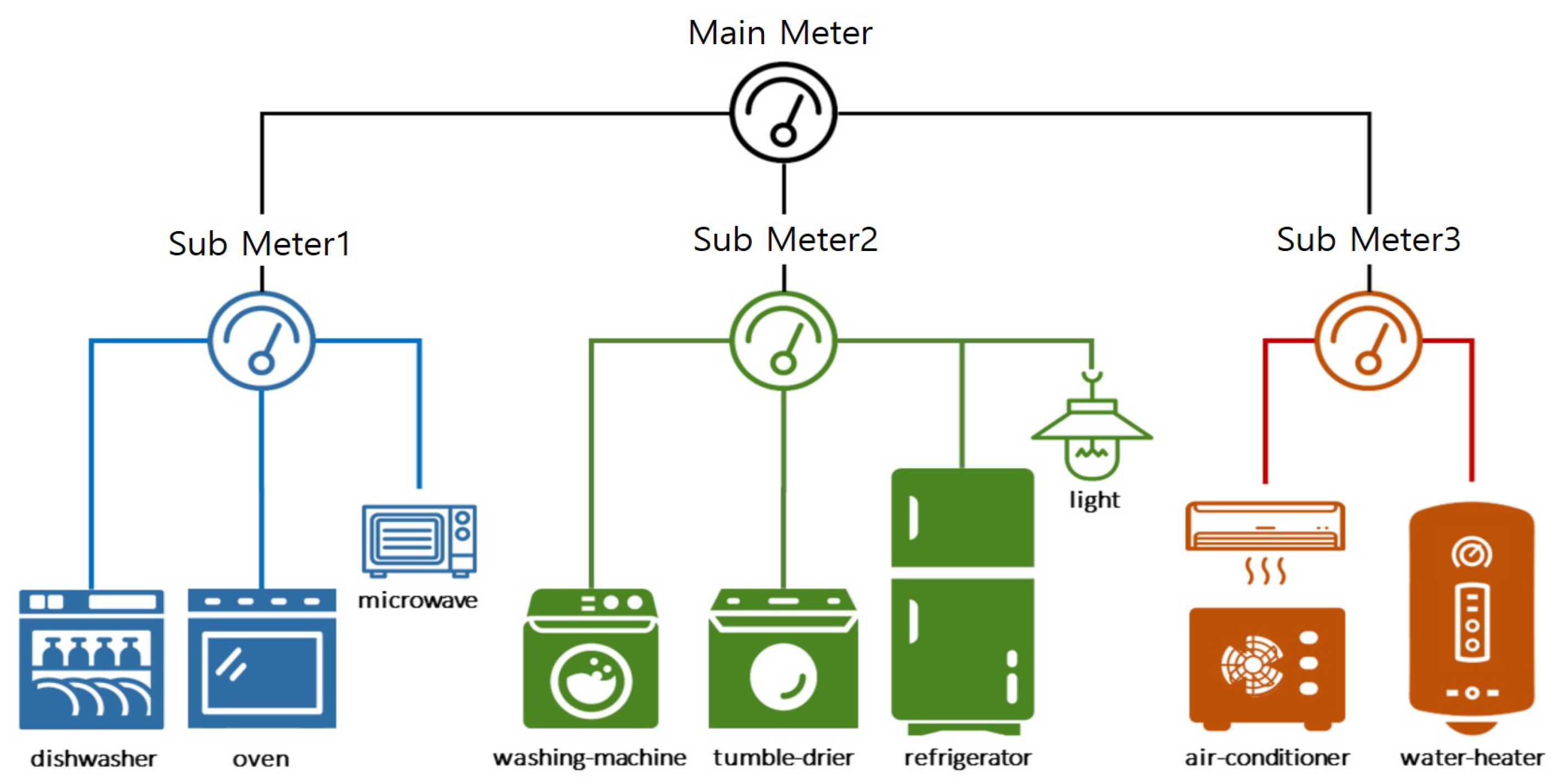
In this section, we review the concepts of NILM and the literature related to our work. Figure 1 presents some basic concepts of NILM. The appliances in the household are connected to the sub-meters, which are linked to the main meter, and these meters can monitor the overall operational events of the appliances. The aggregated power can be represented as follows:
is the total power read from the meter at time t, is the load of a single active appliance i at time t and is a small noise or error term. The NILM technique was first introduced by Hart in 1992 [1], and many studies have been conducted since its introduction, including machine learning-based, deep learning-based, and spectral graph-based research. In general, deep learning and machine learning-based approaches exhibit effective performance in load classification.
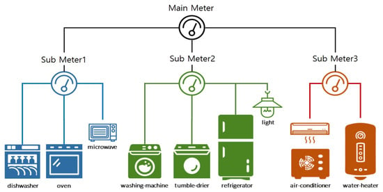
Figure 1.
A Non-Intrusive Load Monitoring (NILM) system [18]. Reprinted from ref. [18].
Numerous machine learning algorithms have been applied to NILM, including the Support Vector Machine (SVM) [2,3], k-Nearest Neighbors (k-NN) [3,4,5], and Hidden Markov Model (HMM) [6,7,8,9,10] algorithms, which are well-known machine learning algorithms that have achieved high performance. However, these traditional machine learning techniques exhibit several limitations in NILM. In the SVM, the classes in the classification are normally restricted to two, which can be increased by applying non-linearity.
However, the increased computational complexity will be a problem when training with a larger dataset [19]. The k-NN algorithm is not efficient in recognizing new appliances. Moreover, as the number of classes increases, the classification accuracy of the method decreases [20]. Finally, in the HMM, the entire structure must be retrained if a new class is added. Moreover, the computational complexity increases exponentially as the number of appliance classes increases, which restrains the performance of the algorithm [21].
Over the past several years, various issues in NILM have been examined using deep learning-based approaches, which have frequently outperformed conventional methods, especially in load classification [22]. Kelly and Knottenbelt [23] proposed three deep neural network architectures to extract operational features from the total power: Long Short-Term Memory (LSTM), Denoising Autoencoders (DAE), and a network called Rectangles. The networks with convolutional layers exhibited superior performance, particularly on unseen data. This means that a convolutional layer is capable of extracting the inherent patterns from the total power. De Baets [15] proposed voltage-current (VI) trajectory images that were weighted and reformed for appliance recognition.
De Baets used a simple and light CNN architecture, and the approach achieved novel results overall for a large number of appliances. Subsequently, Concatenate-CNN and spectrogram images that were preprocessed by Short-Time Fourier Transform (STFT) were suggested to eliminate noise and background loads from the target appliance to improve the classification performance. The results demonstrated that Concatenate-CNN outperformed the methods of previous works [11].
However, the above image-based approaches only consider the operational events of appliances without temporal characteristics, which is an important factor for making the on–off events more valuable. The concatenate-CNN and spectrogram image approach were tested primarily in single-load cases. Thus, the results in the paper [11] are not guaranteed in multi-load classification using this technique. In contrast, the method proposed in this paper can easily patternize the temporal features of the total power, which is the sum of the operational patterns, and CNN can capture the features in the created pattern. Moreover, the method can be used effectively in multi-load as well as single-load cases.
3. Temporal Bar Graph
We propose a temporal bar graph transformation, which patternizes the power signature in the time sequence. This transformation converts original time series data to a sequence of graphs. Each graph represents a temporal pattern of data in a specific time window, and this can be adopted in the training of various image-based deep learning techniques.
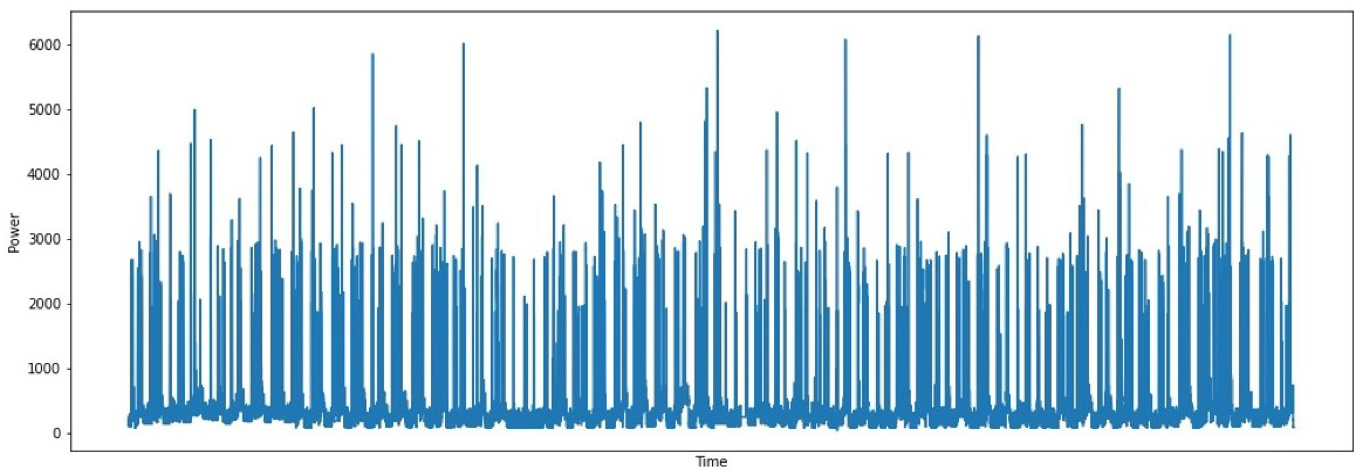
Our main idea of the temporal bar graph is as follows. Figure 2 shows the power signature in a time sequence. Whenever an appliance is switched on or off, the power signal moves up or down with the power signature below. Apart from on–off events, no further useful features can be visually observed. With on–off events solely, it is difficult to identify which appliance is turned on or off particularly when several appliances are activated at the same time. Hence, the enhancement of the performance in load classification is limited with the on–off events especially in the multi-load case.
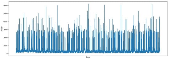
Figure 2.
A power signature in a time sequence.
To address these limitations of using the on–off status, we propose the temporal bar graph. First of all, the temporal bar graph is converted from power signal as shown in Figure 3 and offers an advantage in single-load and multi-load classification since the bar graph patternizes on–off events and the operational times together. This means that the temporal bar graph reorganizes the features of the on states as well as off states and determines how long the on and off states last. Below, we explain the details of the temporal patternization.
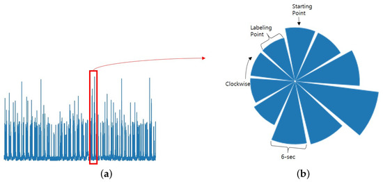
Figure 3.
Power signal (a) transformed into a temporal bar graph (b).
The temporal bar graph consists of 10 bars in this paper. Each bar has 6 s of temporal features. Therefore, one temporal bar graph has 60-s temporal features and appliance usage patterns. The time gap of 6 s in this paper can be changed depending on the domains or experimental circumstances. The length of a bar expresses the amount of energy consumption, with a longer bar indicating that more energy is consumed. Every bar graph is labeled at the Labeling Point, which is the last point among 60-s data, and the starting point is next to the Labeling Point bar as shown in Figure 3.
The starting and labeling points are automatically set since the first data point becomes the starting point and the last data point becomes the labeling point when the graph is generated.
Thus, rotating or pivoting of the graph does not change the starting and labeling points and consequently, it does not lead to performance degradation. When the last point is labeled, it refers to the history of nine previous statuses, and, as the labeling is carried repeatedly, the labeling becomes the usage patterns in the time sequence. Therefore, the temporal bar graph itself becomes a combination of operational features and time characteristics. We call this temporal patternization. Subsequently, a convolutional layer can efficiently detect and obtain meaningful patterns by managing the weights of each bar. For convolutional layers, each 60-s bar graph is transformed into an image for the input data.
Figure 4 depicts two representative graphs of five appliances in a single load: Dish Washer (DW), Kettle, Washing Machine (WM), Microwave (MW), and Fridge. DW and Fridge in Figure 4a,e exhibit round patterns, Kettle and MW in Figure 4b,d exhibit fan-shaped patterns, and WM in Figure 4c exhibits square-like patterns. Figure 5 represents temporal bar graphs in a multi-load combination (MW + WM). Figure 5a shows a pattern in which both MW and WM are not activated. However, the round shape and the graph size that exhibits the level of power consumption are somewhat similar to Figure 4e, and we can assume that the Fridge is operated in Figure 4a.
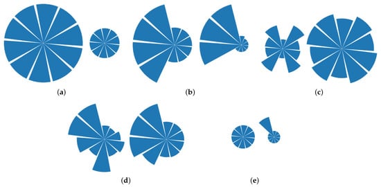
Figure 4.
Characteristics of the temporal bar graph patterns with a single load. (a) DW, (b) Kettle, (c) WM, (d) MW, and (e) Fridge.

Figure 5.
Representative temporal bar graph patterns in a multi-load combination (MW + WM). (a) Both appliances are off, (b) WM is on, (c) MW is on, and (d) Both appliances are on.
Likewise, Figure 5b,c are analogous with Figure 4c,d since these graphs were made from the same appliance usage patterns. When MW and WM are working together, the shape of a graph is more likely to be a combined form Figure 4c,d. Figure 5d is similar to the combined form. Naturally, these shapes depend on the operational characteristics of the appliance and the usage routines of its user. If the bar graph shape is analogous to a shape of another bar graph in certain periods, we consider these two patterns as the same usage patterns to enhance the model performance during training. If the graph is converted into an image, the proposed concept offers the advantage of energy management of the features, which can be extracted efficiently using deep learning techniques, including CNNs.
Two representative image-based approaches using deep learning methods exist: the spectrogram and VI trajectory. These methods preprocess high frequency data and transform the preprocessed data into images for appliance classification. Hence, the classification performance is highly affected by the data preprocessing and the time-series characteristics, which can be useful as the operational patterns are not considered important in these approaches when the data are converted into the image.
However, the proposed method does not require complicated preprocessing and provides a graphical visualization that is understandable by sight. Moreover, our method is advantageous for extracting the detailed patterns of a power signature because it patternizes the operational patterns and temporal features together. The simple application of our approach to raw data can enhance the load identification performance for both single and multiple loads.
4. Experiments
In this section, we demonstrate the performance of the proposed temporal bar graph on state-of-the-art deep learning techniques, namely the VDOCNN and Xception. To verify the proposed approach, experiments were conducted using three cases: (1) a single-load performance comparison between the original current data (raw data) and the bar graph; (2) a multi-load performance comparison between the raw data and bar graph; and (3) a performance comparison of the bar graph with the spectrogram.
4.1. Dataset and Data Preprocessing
The UK Domestic Appliance-Level Electricity (UK-DALE) [24] dataset was used to confirm that the application of the bar graph could enhance the classification performance based on the same models and data. The UK-DALE dataset consists of five UK houses. The mains in each house were sampled at 1 Hz, and the data were measured every 6 s. The total duration of the five houses was 786 days, and the total number of appliances was 54. Houses 1, 2, and 5 were selected for our experiments because they had more realistic power signals. We used House 1 as training data and Houses 2 and 5 as test data. The House 1 data from 01-01-2014 to 11-01-2014 (11 days, date in the format DD-MM-YYYY) were used as the training dataset, whereas the House 2 data from 20-05-2013 to 31-05-2013 (11 days) and the House 5 data from 29-06-2014 to 10-07-2014 (11 days) were used as the test datasets.
The Tracebase dataset was sampled at 1 Hz, and the data points were measured every 1 s from German households. This did not contain the aggregated power. In our experiments, we used the sum of the power consumption of selected appliances as the aggregated power. The total duration of the data was 1883 days with 43 different types of appliances. We used the complete data of Tracebase and chose 7 days where there were the five appliances in common. Table 1 shows the number of events of UK-DALE and Tracebase in the training and test sessions.

Table 1.
The number of events in the training and test datasets.
In each of the above datasets, we chose the following five common appliances for our experiments: Fridge, Washing Machine (WM), Dish Washer (DW), Kettle, and Microwave (MW). These five appliances were selected since they were present in the three houses of UK-DALE and Tracebase. Additionally, the five appliances are commonly used for evaluating NILM methods [25]. Each 60-s temporal bar graph was converted into an image for the input data since a convolutional layer can efficiently extract the useful features from a graph image. For 60-s intervals, we used 10 data points for UK-DALE and 60 data points for Tracebase.
The detailed procedure of generating a temporal bar graph for single cases was as follows:
- 1.
- The total power is sliced into 60-s intervals.
- 2.
- Each sliced interval of the data is labeled by the activation status of each single appliance on the last data among the 60-s points, and labeling is based on the threshold listed in Table 2.
 Table 2. Threshold of the appliances.
 - 3.
- the largest value among the entire dataset is the maximum value, and the minimum value is set to 0.
- 4.
- Each labeled interval is converted into temporal bar graph images with size.
The procedure of generating a temporal bar graph for multi-load cases is as follows:
- 1.
- The total power is sliced into 60-s intervals.
- 2.
- Each sliced interval of the data is labeled by the activation status of the appliances on the last point. For instance, in the DW+Fridge case, when both appliances are not activated on the last point, the label will be 0, and, when only DW is activated on the last point, the label will be 1. Likewise, when only Fridge is operational on the last point, the label will be 2, and when both appliances are operational on the last point, then the label will be 3. The three and five combinations are labeled in this way on the basis of the operational threshold listed in Table 2 and the graph images are generated for the different combinations.
- 3.
- Set the largest value among the entire set of data points as the maximum value, and the minimum value is set to 0.
- 4.
- Each labeled interval is transformed into graph images with the size of .
We determined the ON () and OFF () states of the appliances by using the operational threshold q of each appliance and the total power , as indicated in Table 2. Note that is equivalent to , and is for each appliance.
4.2. Experimental Setup
Every experiment in this study was carried out using the TensorFlow framework and Keras. The learning rate and optimizer were and Adam, respectively. For the loss function, we used binary cross-entropy in the single-load case and categorical cross-entropy in the multi-load case. The configuration for the experiments was as follows:
- CPU: Intel(R) Core(TM) i7-9700K CPU @ 3.60GHz
- RAM: 64 GB
- GPU: GeForce GTX 2080 Ti
- OS: Windows 10.
4.3. Evaluation Metrics
True positive (TP) was indicated when the working state of an appliance was classified as ON. True negative (TN) was stated when the not-working state was classified as OFF. False positive (FP) was indicated when the not-working state was classified as ON. False negative (FN) was stated when the working state was classified as OFF. The Precision, Recall, F1-score, and Accuracy were used for evaluation in this study and are defined as follows:
4.4. Network Architecture
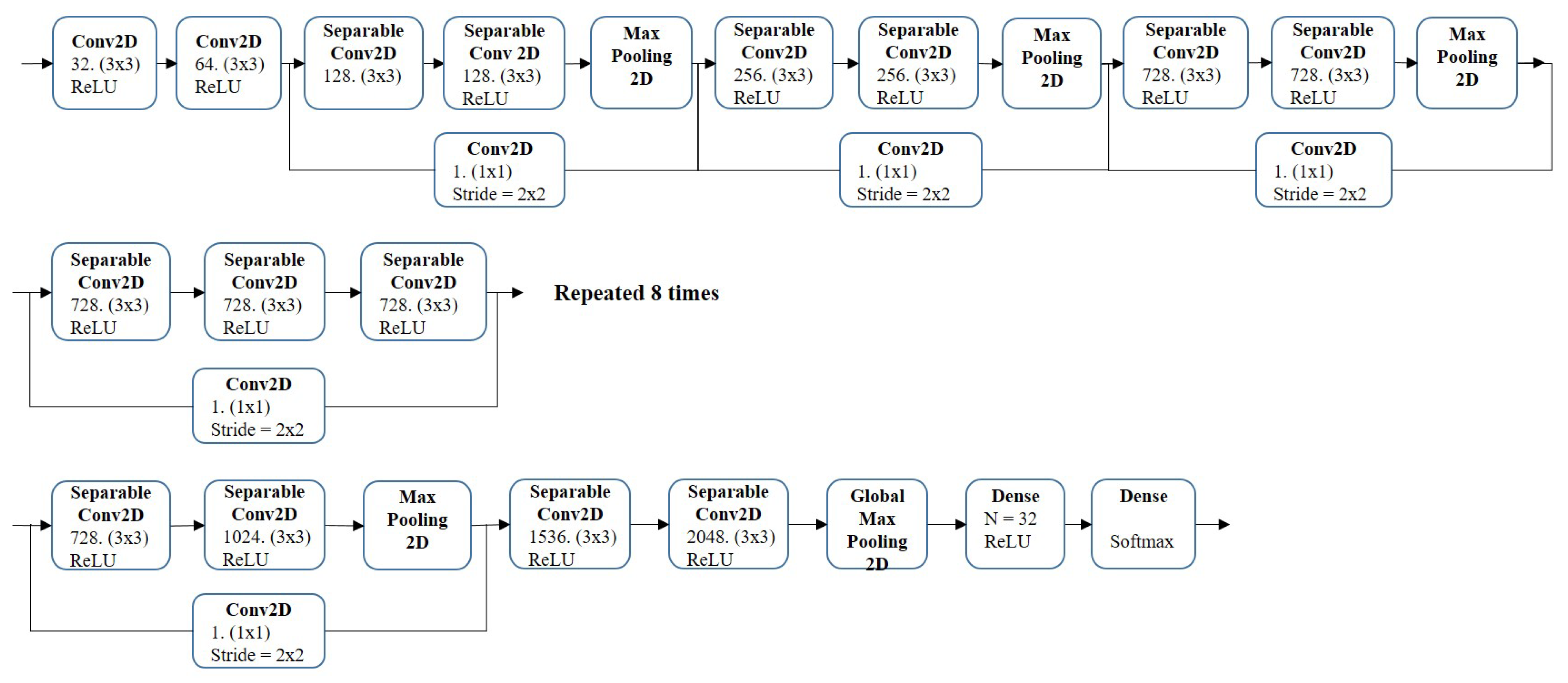
VDOCNN [16] and Xception [17] are commonly used CNN architectures that yield state-of-the-art performance in image classification tasks. We deployed VDOCNN, which consists of a 1-dimensional (1D) convolutional layer, as illustrated in Figure 6 and Xception, which consists of a 2-dimensional (2D) convolutional layer, as depicted in Figure 7. The reason for selecting VDOCNN and Xception is that they are state-of-the-art networks consisting of 1D and 2D convolutional layers and show a solid performance in the image classification tasks. We can evaluate that our method showed stable performance on the dimension changes of the convolutional layers.

Figure 6.
The network architecture of VDOCNN.
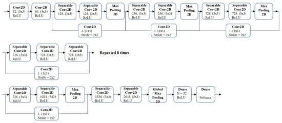
Figure 7.
The network architecture of Xception.
VDOCNN is a 1-dimensional convolutional neural network that can efficiently conduct 2-dimensional image classification tasks. However, there will be some missing values since VDOCNN converts 2-dimensional data to 1-dimensional data. Xception is motivated by the Inception model and showed more efficient performance over the Inception network on the ImageNet dataset. Specifically, 1 × 1 convolutional layers in Inception were replaced with 3 × 3 convolutional layers, and more 3 × 3 layers were added in the Xception model. Xception considerably reduced the convolutional computing cost. However, only a few performance demonstrations are reported since it is a new model.
5. Results and Discussion
5.1. Raw Data and Temporal Bar Graph
5.1.1. Single Load
In this experiment, we compared the accuracy and F1-score of appliances using raw data (without our method), which were the original signal data and the graphs (with our method) on VDOCNN and Xception. As the images are 2D, we converted the graph images into 1D vectors in this experiment to verify that the innate patterns in the graph images did not disappear. We used the array method in the NumPy library to convert 2D graph images into 1D vectors.
Table 3 indicates that the proposed approach moderately enhanced the performance of the VDOCNN model on Tracebase, and our method slightly reduced the performance of VDOCNN on UK-DALE. In detail, for UK-DALE, Kettle and WM showed a slight enhancement in performance while DW, Fridge, and MW recorded slight decreases in performance. For Tracebase, although DW and Fridge showed huge performance improvements, Kettle and WM exhibited slight reductions in performance. On average, the proposed method improved the performance. Table 4 shows that the bar graph resulted in higher scores, especially for Fridge, on the Xception model in UK-DALE and Tracebase.

Table 3.
The results of a single appliance with VDOCNN.

Table 4.
The results of a single appliance with Xception.
When 2D image data were embedded into 1D vectors, data and feature loss was unavoidable. Accordingly, this loss can negatively affect the performance. Likewise, since the 2D graph images were embedded into 1D vectors and we used 1D convolutional layers (VDOCNN), we expected a decline in performance. However, the Accuracy and F1 score were only dropped by 0.2% each on UK-DALE. On the other hand, the scores were increased by 3.18% and 3.17% each on Tracebase as listed in Table 3. Conversely, when 1D raw data were converted into 2D data, the scores often dropped in single and following multi-load cases. A comparison of the results in Table 3 and Table 4 supports that the loss derived from embedding can cause a performance decrease.
We tested on VDOCNN to confirm the robustness in dimensional changes. Even though our method slightly decreased the scores on UK-DALE in the VDOCNN model, we checked that the most inherent features in the graphs did not disappear after the 1D embedding.
According to the tests, the bar graph was robust to the dimensions of the convolutional layers and input data, which indicates that the bar graph retained the innate patterns even if the dimensions of the data were changed. Correspondingly, we could confirm the performance improvement of the networks when applying the bar graph in the single-load case.
5.1.2. Combination of Two Appliances
In this experiment, we investigated a combination of two appliances on the VDOCNN and Xception networks. Table 5 displays the results of the mixed load of two appliances with the VDOCNN. Without the proposed approach, in UK-DALE, the accuracy and F1-score decreased by 9.26% and 9.32%, respectively, whereas, with the proposed method, the scores decreased by only 4.46% and 4.28%, respectively, compared to the results of the single-load case. In Tracebase, the scores slightly increased with our method by 1.04% and 1.35%. The bar graph exhibited a significant improvement in the Fridge + WM case with UK-DALE and Tracebase.

Table 5.
The results of combinations of two appliances with VDOCNN.
Table 6 presents the results of the two appliances with Xception. Without the proposed method, in UK-DALE, the accuracy and F1-score decreased by 13.91% and 15.15%, respectively, whereas, with the proposed method, the scores decreased by 8.32% and 8.47%, respectively, compared to the single-load results. In Tracebase, with our method, the scores dropped by only 0.15% and 0.2%, respectively. In the MW + Fridge case, the results without our method exhibited poor performance in UK-DALE and Tracebase, while the bar graph shows superior performance in the MW + Fridge tests in both datasets.

Table 6.
The results of combinations of two appliances with Xception.
The overall F1-score and accuracy were reduced compared to those of the single-load case because an additional appliance was added. However, the scores of the bar graph were observed to be higher and more stable compared with those of the raw data.
5.1.3. Combination of Three Appliances
In this experiment, a combination of three appliances was tested on the VDOCNN and Xception models. Without our method, in UK-DALE, the accuracy and F1-score decreased by 11.37% and 11.41%, respectively, whereas, with our method, the scores decreased by 13.80% and 13.68%, respectively, compared to the scores of the two-appliance case on VDOCNN as indicated in Table 7. In Tracebase, the scores with our method were higher than the scores without our method.

Table 7.
The results of combinations of three appliances with VDOCNN.
On Xception with UK-DALE, the accuracy and F1-score decreased by 12.32% and 11.24%, respectively, for the raw data, whereas the scores decreased by 11.05% and 11.01%, respectively, for the bar graph compared to the results of the two-appliance case, as reported in Table 8. In Tracebase, the scores decreased only 1.2% each. The graph exhibits improved performance in several tests on both networks, such as DW + Fridge + Kettle, DW + Fridge + MW, DW + Fridge + WM, DW + Kettle + MW, and Fridge + MW + WM in UK-DALE and Tracebase. However, there are some cases where our method showed the worse performance on VDOCNN with Tracebase, such as Fridge + Kettle + MW, Fridge + Kettle + WM, and Fridge + MW + WM, as listed in Table 7. As in the previous cases, the 1D embedding of data can negatively affect the performance.

Table 8.
The results of combinations of three appliances with Xception.
Compared to the combination of two appliances, the average F1-score and accuracy were reduced as one more appliance was included. However, the application of the bar graph still outperformed the results of the raw data in UK-DALE and Tracebase.
5.1.4. Combination of Five Appliances
In this experiment, we examined a combination of five appliances with VDOCNN and Xception for the UK-DALE and Tracebase datasets. The results are shown in Table 9, Table 10, Table 11 and Table 12. The results show that our method significantly improved over all the baselines in terms of the accuracy, F1-score, recall, and precision. On the VDOCNN with UK-DALE, the accuracy and F1-score for the raw data decreased by 15.72% and 15.62%, respectively, whereas the scores for the bar graph decreased by 8.74% and 8.35%, respectively, compared to the results of the three appliances case.

Table 9.
The results of combinations of five appliances with VDOCNN (UK-DALE).

Table 10.
The results of combinations of five appliances with VDOCNN (Tracebase).

Table 11.
The results of combinations of five appliances with Xception (UK-DALE).

Table 12.
The results of combinations of five appliances with Xception (Tracebase).
In Tracebase, the scores increased by 2.38% and 3.88% with the proposed method. For Xception with UK-DALE, the accuracy and F1-score decreased by 30.22% and 30.91%, respectively, for the raw data, whereas the scores for the bar graph decreased by 8.74% and 6.99%, respectively, compared to the results of the three appliances test. In Tracebase, the scores decreased 5.85% and 3.17% with the proposed approach.
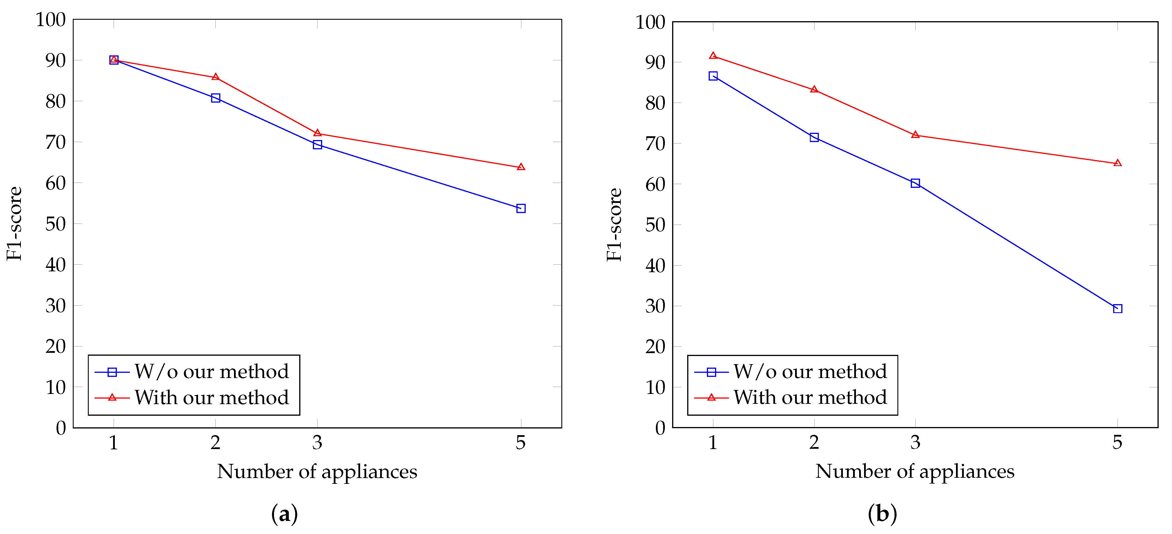
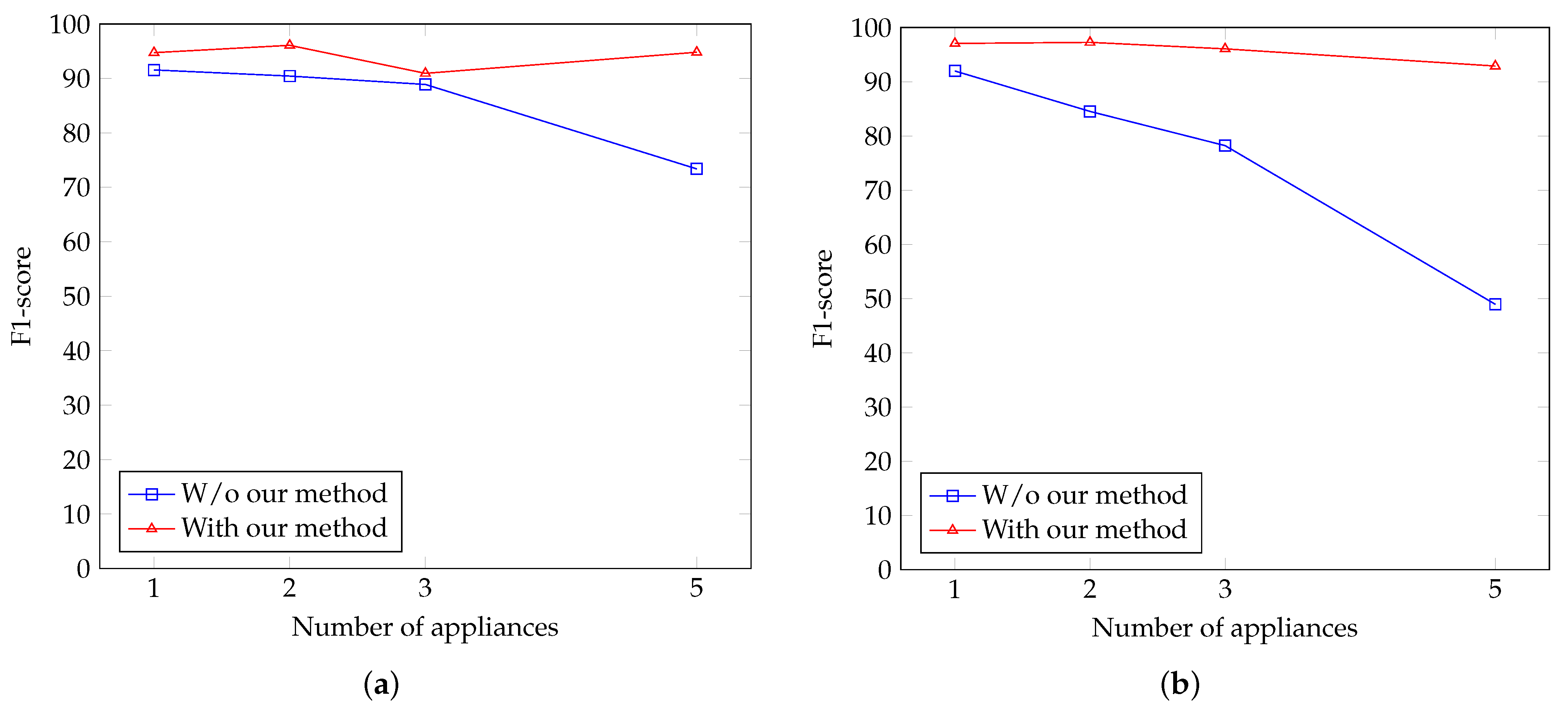
Overall, we conducted tests on a single appliance as well as on combinations of two, three, and five appliances. The results verified that the performance of the two models was improved by implementing the proposed approach, as illustrated in Figure 8 and Figure 9. The figures indicate that the performance gap between with and without our method increased as the number of appliances increased, and the gap reached the maximum value in the five-appliance case. Therefore, if various commonly used appliances are operating simultaneously, simply applying the bar graph to the raw data can make the models more efficient, leading to enhanced performance.
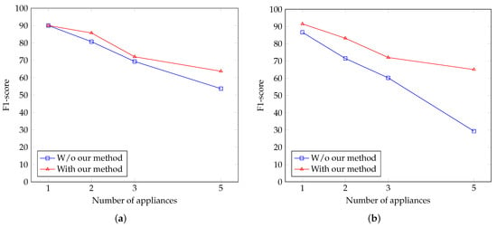
Figure 8.
The F1-score corresponding to the number of appliances on UK-DALE with the (a) VDOCNN model and (b) Xception model, respectively.
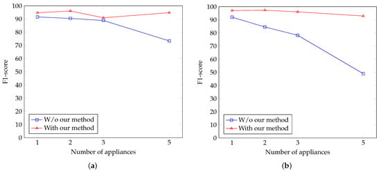
Figure 9.
The F1-score corresponding to the number of appliances on Tracebase with the (a) VDOCNN model and (b) Xception model, respectively.
5.2. Spectrogram and Temporal Bar Graph
In this experiment, we compared the temporal bar graph with the spectrogram on Concatenate-DenseNet121 [11], which has previously exhibited strong performance in image classification tasks. We selected the spectrogram method because it is a state-of-the-art image-based approach. The size of the spectrogram images in this test was , and the images were preprocessed by STFT for feature exposure. An image consisted of 10 data points, which were 60-s long, and it was labeled following the final (10th) data point.
The preprocessing procedure was the same as that of the bar graph image. We selected House 1 and used data from 15-03-2014 to 20-03-2014 (5 days) for training and data from 19-04-2014 to 23-04-2014 (4 days) for testing. The number of images for training and testing were 5900 and 3000, respectively.
The structure of Concatenate-DenseNet121 is shown in Figure 10. The background features and mixed features in Figure 10 were extracted from an embedded network, which is denoted as DenseNet121 in this paper. The results for between the spectrogram and graph are listed in Table 13. Four appliances exhibited slight improvements: DW, Fridge, Kettle, and MW. Although the spectrogram achieved a higher score in the WM test, the graph exhibited an improvement in the overall scores. Thus, we can confirm that the graph provided superior performance compared to the spectrogram.
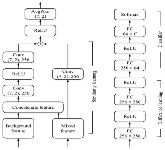
Figure 10.
The network architecture of Concatenate-DenseNet121 [11]. Reprinted from ref. [11].

Table 13.
The results with Concatenate-DenseNet121.
5.3. Comparison with State-of-the-Art Techniques
To validate the proposed method, the F1-scores of other recent deep learning methods using the UK-DALE dataset were compared as listed in Table 14. However, direct comparisons between the results should be carefully conducted since all the experimental configurations were different. In comparison with the latest deep learning techniques, the proposed method showed the highest F1-score among the deep learning methods using low frequency data with regard to appliance identification, and this indicates that the convolutional layers actually detected our temporal patternization and extracted useful features from the patterns.

Table 14.
The performance of the appliance classification on the UK-DALE dataset.
6. Conclusions
In this paper, we proposed a novel approach for improving the classification of operating appliances with temporal patterns using the bar graph. We demonstrated its usefulness through experiments with single and multiple loads. The proposed method was robust to network structures and the dimension reduction of data, and we confirmed that the temporal patternization actually contributed to enhancing the NILM performance. Additionally, our method can be broadly applied to other image-based temporal topics, and other papers dealing with application classification could be improved by applying our method. However, further verification using more datasets and appliances is required to disaggregate real-world data and to determine a means of applying the method in more complicated situations.
We will conduct further research on approaches using images in appliance classification and will compare the advantages and disadvantages of the techniques. We will continue to identify state-of-the-art approaches in artificial intelligence to determine better solutions for NILM issues.
Author Contributions
Conceptualization, H.K. and S.L.; methodology, H.K. and S.L.; software, H.K.; validation, H.K. and S.L.; formal analysis, H.K. and S.L.; investigation, H.K. and S.L.; resources, H.K.; data curation, H.K.; writing—original draft preparation, H.K.; writing—review and editing, S.L.; visualization, H.K. and S.L.; supervision, S.L.; project administration, S.L.; funding acquisition, S.L. All authors have read and agreed to the published version of the manuscript.
Funding
This work was supported by a research fund of Chungnam National University.
Institutional Review Board Statement
Not applicable.
Informed Consent Statement
Not applicable.
Data Availability Statement
Not applicable.
Conflicts of Interest
The authors declare no conflict of interest.
References
- Hart, G.W. Nonintrusive Appliance Load Monitoring. Proc. IEEE 1992, 80, 1870–1891. [Google Scholar] [CrossRef]
- Hassan, T.; Javed, F.; Arshad, N. An empirical investigation of VI trajectory based load signatures for non-intrusive load monitoring. IEEE Trans. Smart Grid 2013, 5, 870–878. [Google Scholar] [CrossRef]
- Figueiredo, M.B.; De Almeida, A.; Ribeiro, B. An experimental study on electrical signature identification of non-intrusive load monitoring (nilm) systems. In Proceedings of the International Conference on Adaptive and Natural Computing Algorithms, Ljubljana, Slovenia, 14–16 April 2011; Springer: Berlin/Heidelberg, Germany, 2011; pp. 31–40. [Google Scholar]
- Kramer, O.; Wilken, O.; Beenken, P.; Hein, A.; Hüwel, A.; Klingenberg, T.; Meinecke, C.; Raabe, T.; Sonnenschein, M. On ensemble classifiers for nonintrusive appliance load monitoring. In Proceedings of the International Conference on Hybrid Artificial Intelligence Systems, Salamanca, Spain, 28–30 March 2012; Springer: Berlin/Heidelberg, Germany, 2012; pp. 322–331. [Google Scholar]
- Giri, S.; Bergés, M.; Rowe, A. Towards automated appliance recognition using an EMF sensor in NILM platforms. Adv. Eng. Inform. 2013, 27, 477–485. [Google Scholar] [CrossRef]
- Wong, Y.F.; Şekercioğlu, Y.A.; Drummond, T.; Wong, V.S. Recent approaches to non-intrusive load monitoring techniques in residential settings. In Proceedings of the 2013 IEEE Computational Intelligence Applications in Smart Grid (CIASG), Singapore, 16–19 April 2013; pp. 73–79. [Google Scholar]
- Aiad, M.; Lee, P.H. Non-intrusive load disaggregation with adaptive estimations of devices main power effects and two-way interactions. Energy Build. 2016, 130, 131–139. [Google Scholar] [CrossRef]
- Cominola, A.; Giuliani, M.; Piga, D.; Castelletti, A.; Rizzoli, A.E. A hybrid signature-based iterative disaggregation algorithm for non-intrusive load monitoring. Appl. Energy 2017, 185, 331–344. [Google Scholar] [CrossRef]
- Kong, W.; Dong, Z.Y.; Hill, D.J.; Ma, J.; Zhao, J.; Luo, F. A hierarchical hidden Markov model framework for home appliance modeling. IEEE Trans. Smart Grid 2016, 9, 3079–3090. [Google Scholar] [CrossRef]
- Mueller, J.A.; Kimball, J.W. Accurate energy use estimation for nonintrusive load monitoring in systems of known devices. IEEE Trans. Smart Grid 2016, 9, 2797–2808. [Google Scholar] [CrossRef]
- Wu, Q.; Wang, F. Concatenate convolutional neural networks for non-intrusive load monitoring across complex background. Energies 2019, 12, 1572. [Google Scholar] [CrossRef]
- Kim, J.G.; Lee, B. Appliance classification by power signal analysis based on multi-feature combination multi-layer LSTM. Energies 2019, 12, 2804. [Google Scholar] [CrossRef]
- Du, L.; He, D.; Harley, R.G.; Habetler, T.G. Electric load classification by binary voltage–current trajectory mapping. IEEE Trans. Smart Grid 2015, 7, 358–365. [Google Scholar] [CrossRef]
- Gao, J.; Kara, E.C.; Giri, S.; Berges, M. A feasibility study of automated plug-load identification from high-frequency measurements. In Proceedings of the 2015 IEEE Global Conference on Signal and Information Processing (GlobalSIP), Orlando, FL, USA, 14–16 December 2015; pp. 220–224. [Google Scholar]
- De Baets, L.; Ruyssinck, J.; Develder, C.; Dhaene, T.; Deschrijver, D. Appliance classification using VI trajectories and convolutional neural networks. Energy Build. 2018, 158, 32–36. [Google Scholar] [CrossRef]
- Dash, P.; Naik, K. A very deep one dimensional convolutional neural network (VDOCNN) for appliance power signature classification. In Proceedings of the 2018 IEEE Electrical Power and Energy Conference (EPEC), Toronto, ON, Canada, 10–11 October 2018; pp. 1–6. [Google Scholar]
- Chollet, F. Xception: Deep learning with depthwise separable convolutions. In Proceedings of the IEEE Conference on Computer Vision and Pattern Recognition, Honolulu, HI, USA, 21–26 July 017; pp. 1251–1258.
- Puente, C.; Palacios, R.; González-Arechavala, Y.; Sánchez-Úbeda, E.F. Non-Intrusive Load Monitoring (NILM) for Energy Disaggregation Using Soft Computing Techniques. Energies 2020, 13, 3117. [Google Scholar] [CrossRef]
- Kotsiantis, S.B.; Zaharakis, I.; Pintelas, P. Supervised machine learning: A review of classification techniques. Emerg. Artif. Intell. Appl. Comput. Eng. 2007, 160, 3–24. [Google Scholar]
- Guo, G.; Wang, H.; Bell, D.; Bi, Y.; Greer, K. KNN model-based approach in classification. In OTM Confederated International Conferences “On the Move to Meaningful Internet Systems”; Springer: Berlin/Heidelberg, Germany, 2003; pp. 986–996. [Google Scholar]
- Alcalá, J.; Ureña, J.; Hernández, Á.; Gualda, D. Event-based energy disaggregation algorithm for activity monitoring from a single-point sensor. IEEE Trans. Instrum. Meas. 2017, 66, 2615–2626. [Google Scholar] [CrossRef]
- Gopinath, R.; Kumar, M.; Joshua, C.P.C.; Srinivas, K. Energy management using non-intrusive load monitoring techniques-State-of-the-art and future research directions. Sustain. Cities Soc. 2020, 62, 102411. [Google Scholar] [CrossRef]
- Kelly, J.; Knottenbelt, W. Neural NILM: Deep Neural Networks Applied to Energy Disaggregation. In Proceedings of the ACM BuildSys ’15, Seoul, Korea, 4–5 November 2015; pp. 55–64. [Google Scholar]
- Kelly, J.; Knottenbelt, W. The UK-DALE Dataset, Domestic Appliance-level Electricity Demand and Whole-house Demand from Five UK Homes. Sci. Data 2015, 2, 150007. [Google Scholar] [CrossRef] [PubMed]
- Zhang, C.; Zhong, M.; Wang, Z.; Goddard, N.; Sutton, C. Sequence-to-Point Learning with Neural Networks for Non-Intrusive Load Monitoring. In Proceedings of the AAAI ’18, New Orleans, LA, USA, 2–7 February 2018; pp. 2604–2611. [Google Scholar]
- Kahl, M.; Kriechbaumer, T.; Haq, A.U.; Jacobsen, H.A. Appliance classification across multiple high frequency energy datasets. In Proceedings of the 2017 IEEE International Conference on Smart Grid Communications (SmartGridComm), Dresden, Germany, 23–27 October 2017; pp. 147–152. [Google Scholar]
- Kim, J.; Kim, H. Classification performance using gated recurrent unit recurrent neural network on energy disaggregation. In Proceedings of the 2016 IEEE International Conference on Machine Learning and Cybernetics (ICMLC), Jeju, Korea, 10–13 July 2016; Volume 1, pp. 105–110. [Google Scholar]
Publisher’s Note: MDPI stays neutral with regard to jurisdictional claims in published maps and institutional affiliations. |
© 2021 by the authors. Licensee MDPI, Basel, Switzerland. This article is an open access article distributed under the terms and conditions of the Creative Commons Attribution (CC BY) license (https://creativecommons.org/licenses/by/4.0/).

