Optimal Control Strategies for Switchable Transparent Insulation Systems Applied to Smart Windows for US Residential Buildings

Abstract

This paper evaluates the potential energy use and peak demand savings associated with optimal controls of switchable transparent insulation systems (STIS) applied to smart windows for US residential buildings. The optimal controls are developed based on Genetic Algorithm (GA) to identify the automatic settings of the dynamic shades. First, switchable insulation systems and their operation mechanisms are briefly described when combined with smart windows. Then, the GA-based optimization approach is outlined to operate switchable insulation systems applied to windows for a prototypical US residential building. The optimized controls are implemented to reduce heating and cooling energy end-uses for a house located four US locations, during three representative days of swing, summer, and winter seasons. The performance of optimal controller is compared to that obtained using simplified rule-based control sets to operate the dynamic insulation systems. The analysis results indicate that optimized controls of STISs can save up to 81.8% in daily thermal loads compared to the simplified rule-set especially when dwellings are located in hot climates such as that of Phoenix, AZ. Moreover, optimally controlled STISs can reduce electrical peak demand by up to 49.8% compared to the simplified rule-set, indicating significant energy efficiency and demand response potentials of the SIS technology when applied to US residential buildings.

1. Introduction

The building sector accounts for about 76% of electricity use and 40% of all U.S. primary energy use and associated greenhouse gas (GHG) emissions, making it essential to reduce energy consumption in buildings in order to meet national energy and environmental challenges [1]. In particular, heating, ventilation, and air conditioning (HVAC) systems are responsible for up to 50% of the US building sector consumption [2], equivalent to 20 quadrillion Btu per year [3]. Building envelope systems including walls, roofs, and windows are the main contributors for both heating and cooling thermal loads of buildings. In particular, windows can influence heating and cooling through heat transfer as well as solar heat gain. Specifically, typical windows even with energy efficient double-pane glazing have an overall heat transmission coefficient (i.e., U-value) that is five to eight times higher than that of opaque walls [4]. Meanwhile, several techniques have been investigated to make the windows more efficient such as tinted, reflective, and low-emissivity glazing materials [5]. Among all those technologies, smart windows—including smart or adaptive glazing materials for windows and dynamic shading devices—suggest the most effective solutions with offering variable optical properties of windows including solar heat gain coefficient (i.e., SHGC) and U-Value [6]. More detailed, smart glazing has been studied with the highest impact, which could control both the light and solar heat flow into and out of buildings while maintaining access to the outdoor views through the glass, thus offering both energetic and aesthetic advantages over static controls, such as blinds or shades [7,8,9]. For instance, Sbar et al. showed that 20% HVAC energy saving could be achieved simply by taking advantages of electrochromic (EC) dynamic windows compared to static low-emissivity windows. More detailed, smart glazing systems could include several technologies such as chromic materials (i.e., electrochromic, photochromic, thermochromic, and gas chromic), liquid crystals (LC), and electrophoretic as well as suspended-particle devices (SPD) [8]. Indeed, electrical powered visible and infrared regulating technologies have been applied to smart windows could be categorized under AC or DC. AC powered smart windows include SPD, LC, and polymer-dispersed liquid crystal (PDLC). DC-powered smart windows consist mainly of EC types [10,11,12,13,14,15,16,17,18,19,20,21].

Dynamic shading devices and adjustable overhangs, on the other side, have been explored in terms of their potential to adjust automatically thermal and optical properties of windows [22]. Firląg et al. conducted a study and analyzed the impacts of control algorithms for dynamic windows on energy savings and shade operations. They reported that site energy savings could be significant and reach as high as 13.0%, that is, a reduction in source energy up to 21.6%, with most of the savings due to thermal cooling reduction [23] for a typical residential dwelling. However, this technology is mostly analyzed and implemented subject to control strategies for the commercial buildings [24,25,26,27]. For instance, Tzempelikos and Shen analyzed and indicated that shading controls can achieve savings ranging from 10.1% to 34.4% in annual source energy consumption for various office room configurations after comparing four dynamic shading controls [28]. More recently, Alva et al. studied façade systems suitable for both daylighting and solar thermal energy harvesting simultaneously by using liquid filled prismatic louvers [29].

In order to further enhance the energy efficiency of buildings, application of optimization techniques has gained a wide interest for designing and operating energy systems, especially in the last decade [30]. Three categories of optimization techniques have been considered for building energy systems including sensitivity and parametric methods, stochastic optimization algorithms, and meta-model approaches [31]. The sensitivity or parametric analyses are based on selecting key variables that affect building energy performance [31,32]. Stochastic population-based optimization methods integrate variable tracking methods such as genetic algorithms (GA), particle swarm optimization (PSO), and other evolutionary algorithms by selecting certain variable-sets automatically to minimize building energy consumption or multiple targets including costs and comfort level besides energy performance. In particular, GA-based optimization techniques have been widely applied to operated building energy systems [33,34,35,36,37]. While this optimization method similar to almost all the approaches may be trapped in local optima, it generally provides sound solutions with acceptable computational efforts [31,38,39]. Finally, the meta-modeling utilizes unified performance forecasting data such as response surface charts, based on statistical approaches to develop relationships between building design and environmental parameters and energy performance indicators [31,40].

In particular, there are several technologies explored to make the windows shadings dynamic, including both internal (i.e., smart glazing systems) and external dynamic shading controls (i.e., dynamic shading devices). Caldas et al. developed an optimization GA-based and assessed the best window size to reduce the loads [41]. Manzan explored using a genetic optimization for an external shading device with the target of reducing the overall primary energy consumption in an office room, while a shading device coupled with different glazing systems resulted in up to 30% reduction of HVAC energy consumption [42]. Moreover, Zhao et al., applied a multi-objective optimization algorithm to minimize the energy use as well as improving the visual and thermal comfort of a reference office room by finding the most appropriate parameters (including size of the window and thickness of the bare glass) for the window system [43]. However, the researchers showed that the objective of energy consumption worsens the visual performance. In addition, Huchuk et al. used a model predictive control (MPC) for interior roller shades using EnergyPlus platform—a state-of-the-art whole building energy simulation tool. The authors showed that the MPC had the potential to achieve annual HVAC energy savings up to 12.49% [44]. Knudsen and Petersen also conducted a research on dynamic solar shading devices to study the economic MPC of space heating as well as dynamic solar shading [26]. They concluded that using this MPC would suggest higher savings compared to the two-step rule set, and results are promising in terms of energy cost as well as peak demand cost.

In this paper, the GA-based optimization approach is applied to operate switchable insulation systems (SISs) both transparent and opaque in order to minimize the energy consumption of US residential buildings. In the literature, adaptive insulation systems have been applied mostly to opaque building envelope elements (i.e., walls and roofs) using several technologies including air flowing within the insulation layers or channels oriented in the direction of heat transfer [45], phase change materials [46], moving insulation sheets [47], and rotating insulation layers [48,49,50,51,52,53]. Recently, Dabbagh and Krarti [53] investigated the use of switchable insulated systems for windows as internal attachments operated using rule-based controls to optimize the overall energy performance of buildings. In this study, novel switchable transparent insulation systems are considered to improve the energy performance of smart glazed windows. First, switchable transparent as well as opaque insulation systems and their operation are briefly outlined. Then, the optimization methodology used to determine the optimal settings for the switchable transparent insulation systems (STIS) applied to smart windows is detailed. Finally, the results of a series of sensitivity analyses are summarized to assess the impacts of optimizing STIS and smart glazing settings on both daily heating and cooling energy consumption and electrical peak demand for representative US residential buildings. Finally, the optimal operation of opaque switchable insulation system (SIS) is considered when applied to conventionally glazed windows.

2. Switchable Insulation Description

The switchable insulation evaluated in this study is based on dynamic insulation systems made up of insulation baffles that can synchronously rotate using a rule-based or optimized set of controls at any desired rotation angle, θ_i, as indicated in Figure 1a when the insulation is opaque applied to a regular window as an interior shade [52,53]. Using results from a laboratory testing, Figure 2 illustrates the R-value variation of the window assembly as a function of the angle θ_i.

Specifically, the configuration considered in this study consists of switchable transparent insulation layers operating as venetian blinds made up of monolithic silica aerogels (MSA) with high transmittance properties for both light and solar radiation [53,54]. As indicated in Figure 1b, the switchable transparent insulation using venetian blinds made up of MSA and applied to a smart glazing window can independently adjust its overall thermal (i.e., R-value) regardless of the solar heat gain coefficient or SHGC of smart glazing. The dynamic transparent insulation can be applied to any type of smart windows as long as the glazing can be switch between a dark state (i.e., with low SHGC) and a clear state (i.e., high SHGC). Other intermediate states for the smart windows can also be considered by the optimization analysis performed for this study.

As part of a comparative analysis, this study evaluates the performance of opaque switchable insulation systems applied as insulated interior shades to conventional windows having static optical properties, as illustrated in Figure 1a.

3. Building Energy Model Description

In this study, the potential benefits of switchable transparent insulation systems (STIS) applied to smart windows operated using optimized controls are evaluated for a detached one-story dwelling as depicted in Figure 3. The main features for the residential building are summarized in

Table 1. Main characteristics of baseline residential building energy model.

Building Characteristics	Detached
Orientation	South
Floor to Ceiling Height	3 m
Floor Area	144 m2
Window Wall Ratio	15%
Windows	Double-glazed wooden window RSI: 0.35 SHGC: 0.4 Window to Wall Ratio: 15%
Floor	Adiabatic
Wall	RSI-2.3 (brick, rigid insulation, gypsum Board, plaster)
Roof	RSI-3.5 (HW concrete, rigid Insulation, membrane, plaster)
Heating Operation	Period: 1 October–30 April: Temperature Set point: 19 °C
Cooling Operation	Period: 1 May–30 September Temperature Set point: 23 °C
Heating and Cooling System	Heating: Gas-Fire Furnace Efficiency: 95% Cooling: Split Air Conditioner COP 3.8 (EER: 13) [55]
Internal Loads	People Power Density: 72 m2/person Lighting Power Density: 6 W/m2 Equipment Power Density: 3 W/m2 Air Infiltration = 5 air change per hour

. In particular, the house is maintained at 23 °C during cooling periods and 19 °C during heating periods. Moreover, operation schedules typical for US single-family homes are considered as shown in Figure 4 for occupancy, lighting, and appliances. The schedules represent fractions of peak values to represent the occupancy level as well as lighting and equipment uses on an hourly basis.

For the baseline housing unit model, a regular double-pane window is considered with an overall thermal resistance set to be RSI-0.35 (i.e., U-value = 2.86 W/m² K) and SHGC of 0.4 in order to meet the building energy-efficiency requirements for all the US climates considered in this study based on the ASHRAE 90.2 standard requirements [55]. When STIS are applied as interior shades to smart glazed windows, the overall thermal resistance of the shade-window system can vary between a low R-value of RSI-0.35 (U-Value = 2.86 W/m²·K) and a high R-value of RSI-1 (U-Value = 1.00 W/m²·K) using the correlation of Figure 2 between the insulation layers angle and R-value. Generally, other high R-value values can be considered depending on the insulation type and thickness used for the shades. Moreover, the window’s smart glazing, in most of this study, can take two states with a low-SHGC of 0.1 and high-SHGC of 0.4. However, other states with SHGC values up to 0.7 are evaluated as part of a sensitivity analysis. Indeed, DeForest et al. [56,57,58,59] evaluated a window with three states and three SHGC levels including dark or tinted glass (SHGC = 0.1), cool or intermediate glass (SHGC = 0.4), and bright or clear glass (SHGC = 0.7).

4. Development of Optimized Control Schemes

The building energy simulation environment used in this study is based on a Resistance–Capacitance (RC) model, as described in details by Dabbagh and Krarti [52] with a specific window model that has been verified against predictions from EnergyPlus. The advantage of this RC-based simulation environment is its ability to model a building envelope (such as windows) with variable thermal and optical properties [52]. The simulation environment includes GA-optimization module as described in the following section.

4.1. Genetic Algorithm Simulation Environment

For this study, the GA optimization is used to determine the best settings for the STIS as well as the smart glazing state. Specifically, a GA-based optimization analysis is considered to establish the angle position of the switchable insulation layers (i.e., R-value) and the clear or dark state of the smart glazing (i.e., SHGC value) in order to minimize a specific cost function used throughout this study, that is, the energy cost for the house.

GA-based optimization approach utilizes a fixed, linear data structure (i.e., a list of variable values), inspired by the biological evolution, and based on the survival of the fittest by maintaining a population of possible solutions of which the poorest performers are eliminated when selecting a new set of generations. This selection is based on randomly evolving solutions using a predefined population size until a final and acceptable solution is reached by successive iterations [43]. For each generation, new potential solutions are selected to form a new population using operators such as mutation rate to maintain population diversity, crossover rate to enlarge the population offspring, and elite count to maintain high performer individuals.

While there are several parameters that can affect the performance of GA-based optimization, the population size and the number of variables that is referred to as nvar are found to have a significant impact in this study, as discussed in Section 6. The two parameters of population size and number of variables are selected after a series of sensitivity analyses to ensure the robustness and the accuracy of the optimization solution. Specifically, the size of the population is correlated to the number of variables considered by the optimization problem. While a larger population size typically leads to more accurate results, it also requires higher computational efforts. As detailed in Section 6, this study utilizes the results of a sensitivity analysis to determine the best set of optimization parameters to be considered for the analysis.

Furthermore, as GA uses a stochastic approach to generate random initial population sets, each optimizations simulation is repeated 10 times, and only the best set of solutions is selected. For a one-day optimization period, the control frequency for the SITS (i.e., nvar) is set to 24. Such a setting allows the model to alter its R-value and SHGC setting per each hour of the day. Even though the optimization analysis is performed for representative days, GA simulations with large populations and a high number of variables have high computational costs.

4.2. Optimization Cost Function

In this study, the objective cost function, f, for the GA-based optimization analysis considered for controlling the STIS-smart window settings is stated by Equation (1) as follows:

$$\mathrm{f} = \min {\sum }_0^{24\mathrm{h}}\left({\mathrm{E}}_{\mathrm{cooling}}{\ast \mathrm{rate}}_{\mathrm{cooling}}+{ \mathrm{E}}_{\mathrm{heating}}{\ast \mathrm{rate}}_{\mathrm{heating}}\right)$$

(1)

where:

■

E_cooling: Cooling thermal loads for each time-step

■

E_heating: Heating thermal loads for each time-step

■

rate_cooling: Cost of electricity for cooling utility (set to be $0.1/kWh in this study)

■

rate_heating: Cost of natural gas for heating utility (set to be $0.03/kWh in this study)

Since GA-based optimization over an entire year is computationally time consuming, the analysis considers only representative days for each season to evaluate the impact of optimal settings on the performance of STIS when applied to smart windows for the house model described in Section 3.

For this study, the building energy model as well as the GA algorithm have been integrated within MATLAB platform [60] to expedite the optimization computational efforts. Furthermore, the number of options for both R-value and SHGC to be optimized, nvar, has a significant impact on the computational cost. Indeed, for one day optimization using hourly analysis, nvar can be as high as 192 when only high and low options are allowed for STIS position and the smart glazing state is considered for each hour assuming all windows in each façade can be operated with the same settings. Lower values for nvar are desired to reduce the computational efforts as outlined in Section 6. In particular, most of the GA-optimization analyses considered in this study limit nvar to 40 with 24 for the R-value of STIS settings and 16 for smart window states (i.e., SHGC values) by maintaining the same values during four-hour periods for each orientation (North, South, West, and East). Moreover, the smart window is assumed to be set to the baseline clear state (i.e., SHGC = 0.4) during the first and last 4 h of the day and does not need to be optimized.

5. Discussion of Results

In this section, the analysis results for GA-based optimization are presented when applied to a house located in Golden, CO, during three representative days including one for the swing season, one for the cooling season, and one for the heating season. First, the performance of the GA optimization is evaluated to select specific parameters for the population size and number of variables to considered throughout the analyses carried out for the study. Then, the GA optimization results are obtained using two approaches: sequentially and simultaneously, the best settings of both STIS and smart glazing. Finally, the performance of the STIS–smart window is assessed for various days using the GA-based optimization results. The upper and lower boundaries of the selected R-value and SHGC are summarized in

Table 2. Upper and lower boundaries for R-value and SHGC applied in GA optimization.

Window Property	Baseline	Lower Boundary	Higher Boundary
R-Value (RSI)	0.34	0.35	1
SHGC	0.4	0.1	0.4

.

5.1. Impact of Optimization Sequence

The settings for both STIS and the smart window can be determine simultaneously or sequentially. In this section, the impact of sequential optimization on the overall energy performance of the house located in Golden, CO is evaluated and compared to the results obtained using a simultaneous optimization. Specifically, three optimization approaches corresponding to various applications and operation modes are conducted for this analysis:

Switchable SHGC only: This case corresponds to optimizing only the state settings for the smart windows. It may also represent the operation of an automated opaque shade applied to conventional windows.

Switchable R-value only: This case addresses the operation of only the STIS while keeping the smart windows at the same state. This option can also represent the operation of opaque switchable insulation applied as shades to conventional windows.

Switchable both R-value and SHGC: This case refers to the simultaneous optimal operation of the STIS as well as of the smart windows. This option is the main configuration evaluated throughout this study.

The results of these three optimizations and operation modes are compared to those obtained when the house has static windows with a fixed U-value and SHGC and without any shades. Figure 5 summarizes the daily energy performance for both static windows and STIS applied to smart windows when the house is located in Golden, CO, USA during a swing day (i.e., 21 May). The selected location for this analysis represents an ASHRAE 5B climate zone (Cool-Dry) correspondent to Dfb in the Koppen climate classification [61,62]. In particular, the savings in both heating and cooling end-uses as well as in overall house electrical peak demand are reported using GA-based optimization as well as two-step rule-set controls for smart windows, which are equipped with switchable transparent insulation compared to the baseline case (static windows with no shades).

As the results of Figure 5 indicate, the maximum HVAC load reduction is achieved when both the R-value and SHGC are simultaneously optimized, reaching as high as 50.2% compared to the baseline. However, GA-based optimization provides almost the same energy savings (49.7%) when only SHGC settings are optimized. On the other hand, when only R-values are optimized, lower energy savings (27.1%) are obtained compared to the simultaneous optimization. However, the performance of STIS associated with controlling only the R-values as well as of smart windows defined by adjusting only SHGC values depend on the season and the operation mode. For instance, the date of 21 May considered in the analysis results of Figure 6 is primarily a cooling day with mild temperatures. Thus, the best option to reduce cooling thermal load for the house is to reduce solar heat gains and thus by adjusting SHGC values rather than R-values. The impacts of various climatic conditions are addressed in the following section.

5.2. Impact of Seasons

In this section, impacts of daily variations of weather conditions for Golden, CO, on the optimally operated STIS–smart windows are investigated. More particularly, three representative days of 21 May, 13 July, and 18 December are selected for Golden, CO, to evaluate the performance of the optimized settings for both STIS and smart windows during swing, summer, and winter seasons, respectively.

5.2.1. Representative Day for the Swing Season

Figure 7 shows the performance of the GA-optimized STIS and smart windows during 21 May, a spring day in Golden, CO, USA representing a mild day. As indicated by Figure 7a, the daily optimized load profile is consistently lower compared to loads obtained using baseline windows and the two-step rule-based controls. This lower thermal load obtained from GA-based optimization is explained as illustrated in Figure 7b showing that optimal settings for the smart windows call for lower SHGC one time-step (4 h) earlier than the two-step controller, resulting in less solar heat gains and consequently lower cooling load for the house. Furthermore, the GA-based optimization set the STIS to its low R-value for a longer period allowing the house to release higher heat gains than the two-step controls.

5.2.2. Representative Day for the Summer Season

Figure 8 compares results of the two-step controller and GA-based optimization to those obtained for baseline case during a summer day (13 July) representing a hot day. As indicated in Figure 8a, the GA-based optimizer provides almost the same thermal load as the rule-based controller. However, the actions for both STIS and smart windows are different for both control options. Indeed, the two-step controller sets STIS at its high R-value and the smart windows at its low SGHC value during the daytime hours to prevent thermal and solar heat gains from entering the house. However, the optimal controls seem to alternate between high and low values for the settings of both STIS and smart windows to balance between solar heat gains and the flow of thermal heat transfer between indoors and outdoors.

5.2.3. Representative Day for the Winter Season

The settings for both GA-based optimizer and the two-step controller for a winter day (18th December) are shown in Figure 9. The need to reduce thermal heat transfer as well as increase solar heat gains for this cold day force both controllers to set the STIS at its high R-value and the smart window at its high SHGC value throughout the day, as depicted in Figure 9b.

5.2.4. Summary of Season’s Impacts

Table 3. HVAC loads for baseline windows and STIS–smart windows applied to a house in Golden, CO for three representative days: 21 May (swing season), 13 July (summer season), and 18 December (winter season) using two control strategies.

Daily HVAC Loads (KWh/Day) and Percentage Savings
	21 May	13 July	18 December
Baseline	15.53	57.61	−76.71
2-Step	9.21	41.22	−61.95
GA	7.73	41.03	−61.95
Energy-Saving GA Compared to Baseline	50%	28.8%	28.8%
Energy-Saving GA Compared to 2-Step	16%	0.5%	0.5%

summarizes the impacts of weather conditions on the performance of both GA-based optimization and two-step controller to operate both STIS and smart windows for a house located in Golden, CO. Specifically,

Table 4. Electrical peak demands for baseline STIS–smart windows applied to a house in Golden, CO for three representative days: 21 May (swing season), 13 July (summer season), and 18 December (winter season) using two control strategies.

Electrical Peak Demand (kW) and Percentage Savings
	21 May	13 July	18 December
Peak Load—Baseline	2.09	3.98	0.21
Peak Load—2-Step	1.63	3.08	0.21
Peak Load—GA	1.51	3.07	0.21
Peak Energy Saving GA Compared to Baseline	27.8%	22.9%	0%
Peak Energy Saving GA Compared to 2-Step	7.6%	0.3%	0%

indicates that the best performance for the STIS and smart windows is achieved during 21st May, a swing season day with mild weather conditions. In all cases, the GA optimizer allows more energy savings that the two-step controller.

Furthermore, both optimal and two-step controllers allow some reduction in electrical peak demand for the house as summarized in Table 4 even though the optimization cost-function calls only for reduction in total daily energy use. Specifically, the highest reduction in electrical peak demand achieved by the GA-based optimization occurs for 21 May, when they drop as high as 27.8% and 7.6% compared to baseline and two-step, respectively.

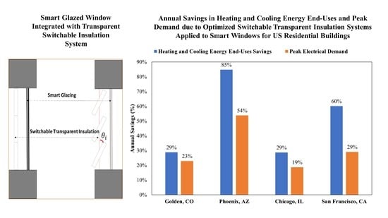
5.3. Impact of Climate

In this section, the performance of GA optimization to operate STIS applied to smart windows is assessed for the houses located in other US locations including Chicago, IL, USA, Phoenix, AZ, USA, and San Francisco, CA, USA representing hot, cold, and moderate climates, respectively, as summarized in

Table 5. Summary of the basic annual characteristics of all the locations used based on International Energy Conservation Code (IECC).

City	Golden, CO, USA	San Francisco, CA, USA	Phoenix, AZ, USA	Chicago, IL, USA
CDD (based on 18 °C)	460	116	2625	505
HDD (based on 18 °C)	3391	1403	593	3596
Climate Type	5B (Cold)	3C (Marine)	2B (Hot-Dry)	5A (Cold)
Average Dry-Bulb Temperature (°C)	9.3	13.3	23.1	9.7
Köppen Climate Classification [61,62]	Dfb	Csb	Bwh	Dfa

.

Table 6. HVAC loads for baseline windows and STIS–smart windows applied to a house located in San Francisco, CA, USA for six representative days using two control strategies.

Daily HVAC Loads (kWh/Day) and Percentage Savings
	21 May	13 July	18 December	11 May	10 July	17 August
Baseline	12.27	25.72	0	20.99	23.26	15.08
2-Step	6.69	12.19	0	11.07	10.47	8.26
GA Optimizer	5.81	10.27	0	9.84	10.27	7.26
Energy Saving GA Optimizer vs. Baseline	52.6%	60.1%	0	53.1%	56%	51.9%
Energy Saving GA Optimizer vs. 2-Step	13.2%	15.7%	0	11.1%	1.9%	12.2%

,

Table 7. Electrical peak demand for baseline windows and STIS–smart windows applied to a house in San Francisco, CA, USA for six representative days using two control strategies.

Electrical Peak Demand (kW) and Percentage Savings
	21 May	13 July	18 December	11 May	10 July	17 August
Baseline	1.61	2.33	1.29	2.14	2.31	1.85
2-Step	1.39	1.69	1.29	1.67	1.68	1.51
GA	1.32	1.66	1.29	1.61	1.66	1.46
Energy Saving GA Compared to Baseline	18%	29.1%	0%	2.14	2.31	1.85
Energy Saving GA Compared to 2-Step	4.9%	2%	0%	1.67	1.68	1.51

,

Table 8. HVAC loads for baseline windows and optimized STIS–smart windows applied to a house located in Phoenix, AZ, USA for six representative days using two control strategies.

Daily HVAC Loads (kWh/Day) and Percentage Savings
	21 May	13 July	18 December	10 July	15 February	15 November
Baseline	60.39	78.56	2.28	77.52	6.04	26.1
2-Step	45.5	61.5	1.91	62.21	4.92	13.74
GA	44.83	61.17	0.35	61.6	3.94	13.38
Energy Saving GA Compared to Baseline	25.8%	22.1%	84.8%	21%	34.8%	49%
Energy Saving GA Compared to 2-Step	1.5%	0.5%	81.8%	77.52	6.04	26.1

,

Table 9. Electrical peak demand for baseline windows and optimized STIS–smart windows applied to a house in Phoenix, AZ, USA—for six representative days using two control strategies.

Electrical Peak Demand (kW) and Percentage Savings
	21 May	13 July	18 December	10 July	15 February	15 November
Baseline	4.16	4.61	0.96	4.44	1.29	2.33
2-Step	3.33	3.92	0.88	3.85	1.22	1.85
GA	3.3	3.91	0.44	3.82	1.12	1.82
Energy Saving GA Compared to Baseline	20.7%	15.1%	53.8%	14%	13.6%	22%
Energy Saving GA Compared to 2-Step	1.1%	0.1%	49.8%	0.9%	8.8%	1.5%

,

Table 10. HVAC loads for baseline windows and optimized STIS–smart windows applied to a house located in Chicago, IL for six representative days using two control strategies (negative sign indicates heating loads).

Daily HVAC Loads (kWh/Day) and Percentage Savings
	21 May	13 July	18 December	1 July	19 September	14 April
Baseline	23.32	37.52	−55.47	26.61	−12.62	−9.27
2-Step	12.55	27.06	−43.93	17.28	−7.26	−7.73
GA	12.32	26.76	−43.93	16.91	−6.16	−5.88
Energy Saving GA Compared to Baseline	47.2%	28.7%	19.7%	36.4%	51.2%	36.6%
Energy Saving GA Compared to 2-Step	1.9%	1.1%	0%	2.1%	15.1%	23.9%

and

Table 11. Electrical peak demand for baseline windows and optimized STIS–smart windows applied to a house in Chicago, IL, USA for six representative days using two control strategies.

Electrical Peak Demand (kW) and Percentage Savings
	21 May	13 July	18 December	1 July	19 September	14 April
Baseline	2.41	2.93	0.21	2.14	1.65	1.7
2-Step	1.9	2.41	0.21	1.81	1.46	1.59
GA	1.88	2.39	0.21	1.78	1.39	1.44
Energy Saving GA Compared to Baseline	21.8%	18.7%	0%	17%	15.6%	15.7%
Energy Saving GA Compared to 2-Step	1%	1%	0%	1.5%	4.7%	9.9%

summarizes the analysis results for both GA-based optimizer and two-step controller for four US locations during six days. The same high and low values for both STIS and smart windows used for Golden, CO, are considered in all climates.

5.3.1. San Francisco, CA, USA

Similar to the trends observed for Golden, CO, USA, the GA-based optimizer to operate the STIS–smart windows outperforms significantly the two-step controller especially during days when the weather conditions are mild. In particular, the GA-based optimizer can reduce during 21st May the HVAC energy use by 60.1% relative to the baseline case and 15.7% relative to the two-step controller. Similarly, the GA optimizer allows a reduction in electrical peak demand estimated to be 4.9% compared to the two-step controls during 21st May, as summarized in Table 6. For San Francisco, most of the days are mild with some cooling needs during the daytime and some heating loads during the nighttime. Thus, the potential for energy savings of the GA-based optimizer is limited, as indicated in Table 6 and Table 7 for electrical peak demand. Figure 10 illustrates the thermal loads as well as the settings for both the GA-based optimizer and the two-step controller for the STIS and smart windows during July 13 when the house is located in San Francisco, CA, USA. While both controls agree for the STIS’ high R-value setting throughout the day, they differ in settings for the smart windows. Indeed, the two-step controls call for a high SHGC setting during the morning hours, while the GA-based optimizer sets the smart windows in its dark state late in the evening, resulting in lower thermal loads throughout the day.

5.3.2. Phoenix, AZ, USA

The performance indicators of STIS–smart windows when applied to a house located in Phoenix, AZ are summarized in Table 8 for HVAC energy use and Table 9 for electrical peak demand during six representative days. The GA-based optimization achieves the highest percent reduction in both HVAC loads and peak demand of respectively 81.8% and 49.8% relative to the baseline case during December 18, which is a relatively cold day in Phoenix, AZ, USA. However, it should be noted that these savings, while significant in terms of percentage, are small in absolute magnitudes due to the low heating loads, as illustrated in Figure 11. Indeed, space heating is needed only in late hours during the day when the outdoor temperature drops, implying that only the SHGC setting can be used by a GA-based optimizer as well as the two-step controller to reduce the HVAC energy use. While the two-step controls call for a low-SGHC setting for the smart windows during the afternoon hours, the optimizer switches back and forth between high and low SHGC settings to maximize the benefits of solar heat gains.

5.3.3. Chicago, IL, USA

When the house is located in Chicago, IL, USA, with a consistently very cold climate throughout the winter, the only opportunities for the STIS–smart windows to reduce the house’s energy use are available during the swing days, as indicated in the results listed in Table 10 for 14th April, 21st May, and 19th September. In particular, the GA-based optimizer provides higher reductions of 36.6% and 23.9% in HVAC energy use compared to respectively the baseline and the two-step controls during 14th April. The specific settings called by a GA-based optimizer and the two-step controls for both the STIS and the smart windows during 14th April are illustrated in Figure 12. The highest peak demand reduction occurs also during mild days, as summarized in Table 11 and reaches up to 21.8% relative to the baseline during 21st May.

6. Sensitivity Analyses

This section presents the results of sensitivity analyses to investigate the impacts of various design specifications, operation conditions, and US locations on the energy performance of STIS applied to smart windows of the prototypical house outlined in Section 3.

6.1. Impact of Optimization Time-Step

In this section, the effect of analysis time-step on the optimization results is discussed. The analysis time-step determines ultimately the number of variables (nvar) to be optimized. Moreover, the analysis time-step can impact the accuracy of the optimization results as well as on the computational efforts.

Table 12. Impact of time-step on optimization results for switchable shades applied to a house located in Golden, CO during 21st May.

Daily HVAC Loads (kWh/Day) and Percentage Savings
	Baseline	2-Step Switchable	GA Optimized 1-h Timestep	GA Optimized 4-h Timestep	GA Optimized 8-h Timestep
HVAC Loads	15.53	9.21	7.70	7.73	7.77
Savings Compared to Baseline	0%	40.74%	50.4%	50.2%	49.9%
Processing Time *	0.3 h	0.3 h	10.4 h	3.5 h	1 h

* For this analysis, the CPU processor consists of an Intel^® Core (tm) i7-8700 with 3.20 GHz.

summarizes the performance of the optimization compared to the two-step controls for 21st May using various time-steps when the house is located in Golden, CO, USA. As the optimization time-step increases, GA-based controls achieve positive but lower energy savings relative to both the baseline and two-step settings. However, the degradation of the optimization results is rather small, but the reduction in computing efforts is significant. Specifically, when the optimization time-step is changed from 1 h to 8 h, the energy savings achieved by the optimization relative to baseline case are slightly reduced from 50.4% to 49.9%, while the computational efforts are decreased from 10.4 h to merely 1.0 h using a 3.30 GHz processor. Indeed, the 1 h time-step optimization must identify the values of 160 variables (i.e., nvar = 160) while only 20 variables (i.e., nvar = 20) when an 8 h time-step is used.

6.2. Impact of Population Size

In this section, the impact of the population size used in the GA optimization analysis is investigated. Generally, the adequate size of the population to achieve accurate optimization results depends closely on the number of variables (nvar) [63]. Specifically, a large population size tends to improve the results’ accuracy but at the expense of higher computational efforts. Hence, a sensitivity analysis is carried out in this section to determine the best set of optimization parameters to be considered for the optimization problem considered in this study. As Nguyen et al. concluded, small population sizes could result in a higher convergence rate of GA algorithms without significant reduction in accuracy levels for some applications [38].

Table 13. Impact of population size on GA optimization results for STIS–smart windows applied to a house located in Golden, CO, during 21 May.

Daily HVAC Loads (kWh/Day) and Percentage Savings
	Baseline	2-Step Switchable both R-Value and SHGC	GA Optimized -Population Size: 50	GA Optimized -Population Size: 100	GA Optimized-Population Size: 200
HVAC Loads	15.53	9.21	7.73	7.74	7.79
Savings Compared to Baseline	0%	40.74%	50.4%	50.4%	49.8%
Processing Time *	0.3 h	0.3 h	3.5 h	5.9 h	10.7 h

* For this analysis, the CPU processor consists of an Intel^® Core (tm) i7-8700 with 3.20 GHz.

summarizes the GA optimization results for various population sizes used to identify the best settings of STIS and smart windows to minimize HVAC energy use for a house located in Golden, CO, USA, during 21st May. The results of Table 13 indicate that when the population size is increased, the energy savings from the GA optimization decrease, while the CPU time increases. Specifically, increasing the population size from 50 to 200 increases the CPU time more than 200% while achieving by 10% lower energy savings. For most of the analyses conducted in this study, the GA population size is set to 50 when the number of variables is less than 40 (i.e., nvar = 40).

6.3. Impact of R-Value and SHGC

The performance of the GA-based optimization of the STIS and smart windows depend on the high/low settings for both the R-value and SHGC value, as evaluated in this section for the case of a house located in Golden, CO, during 21st May. As summarized in Figure 13, the energy-efficiency performance of STIS–smart windows improves with a larger range of high-low operation settings. The increase in the R-value range has more beneficial impacts than the increase of SHGC-value range, especially when optimized controls are used. For instance, when high R-value settings are increased from RSI-1 to RSI-2.5 with the SGHC range kept the same, the HVAC energy savings increased slightly from 50.0% to 50.6%. However, when the high SHGC setting is increased from 0.4 to 0.7 while the R-value range is maintained, the HVAC energy use actually increased due mostly likely to the higher solar heat gains received from the windows as soon as the high SHGC setting is called for.

6.4. Impact of WWR

The impact of increasing WWR on the performance of the GA-based optimizer and two-step controller to operate STIS and smart windows is investigated in this section. Figure 14 outlines the analysis results during 21st May when the house is located in Golden, CO, USA, showing both HVAC loads as well as electrical peak demand and associated savings compared to baseline case. The results imply that increasing the window size (i.e., WWR varying from 30% or 50%) boosts the energy efficiency as well as demand reduction benefits of both STIS and smart windows, especially when operated using optimal controls. Specifically, when the WWR increases to 50%, the STIS–smart windows achieve an HVAC load reduction of 74.5% (i.e., 24.6% vs. the two-step controller), which is higher than 65.9% for WWR = 30%. Moreover, the optimized STIS–smart windows reduce the house electrical peak demand by 57.9% (11.9% vs. two-step controller) for WWR = 50% and by 41.8% for WWR = 30%.

6.5. Impact of Internal Loads

The effects of the internal gains on the performance of STIS–smart windows are summarized in

Table 14. HVAC loads and electrical peak demand for baseline windows and STIS–smart windows applied to a house in Golden, CO, USA—with and without internal loads.

Daily HVAC Loads (kWh/Day) & Electrical Peak Demand (kW) and Percentage Saving
	Baseline (with Internal Loads)	2-Step Switchable (with Internal Loads)	GA Optimized (with Internal Loads)	Baseline (without Internal Loads)	2-Step Switchable (without Internal Loads)	GA Optimized (without Internal Loads)
HVAC Loads	22.43 (0%)	11.17 (50.2%)	9.74 (56.6%)	8.76 (0%)	2.31 (73.7%)	0.62 (93%)
Electrical Peak Demand	2.33 (0%)	1.76 (24.5%)	1.68 (27.8%)	1.11 (0%)	0.36 (67.3%)	0.19 (82.9%)

during 20th September when the house is located in Golden, CO, USA. Specifically, two scenarios are considered for the lighting and equipment loads (with and without) using both the GA-based optimizer and two-step controller to operate the STIS–smart windows. As the results of Table 14 indicate, the absence (or reduced) internal gains enhance the performance of STIS–smart windows, resulting in higher reductions in HVAC loads and electrical peak demand relative to the baseline case especially when optimal setting are used. Indeed, by eliminating or lowering the internal loads, the cooling thermal loads and thus the HVAC energy uses are lowered, leaving mainly the solar heat gains to be managed through the operation of STIS–smart windows. Specifically, HVAC loads can be reduced by 56.6% by GA-based optimized for the case of high internal loads; that is, they are 12.8% better than the two-step controller’s performance. These GA optimizer energy savings increased to 93%, which is 73.3% better than the two-step controller when the internal gains are absent. Indeed, for the case of low internal gains, the baseline HVAC load is small, and therefore, even a low reduction by the optimized controls leads to a higher savings in terms of percentage.

7. Summary and Conclusions

In this paper, the performance of GA-based optimal settings is evaluated to operate switchable transparent insulation systems or STIS combined with smart windows to reduce the HVAC energy use for US residential buildings. It is found that while various parameters can affect its performance, the GA optimizer outperforms the rule-based controls especially for mild climatic conditions. Indeed, the energy-efficiency potential for the STIS and smart windows is high for swing days when the weather is mild with opportunities for both free cooling (night-time) and free heating (daytime). Moreover, the analysis indicates that depending on the house thermal loads and the climatic conditions, the relative importance of settings of STIS or the smart windows may vary. However, the combined effects typically are required to result in the optimal performance for the windows. In particular, the GA-based optimal controls for the STIS and smart windows can achieve over 80% reduction in HVAC energy use for a typical US residential building, especially during mild days. These savings can be higher with larger windows, lower internal gains, and higher R-value settings for STIS. Moreover, it is found that the selection of the high SHGC setting for the smart windows can have a significant impact of the energy efficiency of the residential buildings.

The potential benefits of switchable transparent insulation systems combined with smart window systems or even just switchable opaque insulation applied as venetian blinds to conventional windows can be significantly enhanced through optimal controls using adequate cost functions to provide load flexibility and demand response capabilities. Indeed, the switchable insulation especially when combined with smart windows can provide building demand response features to meet the grid requirements while maintaining acceptable indoor thermal comfort levels.

References

1. US Department of Energy. An Assessment of Energy Technologies and Research: Increasing Efficiency of Building Systems and Technology; US Department of Energy: Washington, DC, USA, 2015.
2. Pérez-Lombard, L.; Ortiz, J.; Pout, C. A review on buildings energy consumption information. Energy Build. 2008, 40, 394–398. [Google Scholar] [CrossRef]
3. U.S. Energy Information Administration. Available online: https://www.eia.gov/energyexplained/us-energy-facts/ (accessed on 17 May 2021).
4. Cho, S.-H.; Shin, K.-S.; Zaheer-Uddin, M. The effect of slat angle of windows with venetian blinds on heating and cooling loads of buildings in South Korea. Energy 1995, 20, 1225–1236. [Google Scholar] [CrossRef]
5. Feng, W.; Zou, L.; Gao, G.; Wu, G.; Shen, J.; Li, W. Gasochromic smart window: Optical and thermal properties, energy simulation and feasibility analysis. Sol. Energy Mater. Sol. Cells 2016, 144, 316–323. [Google Scholar] [CrossRef]
6. Ye, H.; Meng, X.; Xu, B. Theoretical discussions of perfect window, ideal near infrared solar spectrum regulating window and current thermochromic window. Energy Build. 2012, 49, 164–172. [Google Scholar] [CrossRef]
7. Hernandez, T.S.; Alshurafa, M.; Strand, M.T.; Yeang, A.L.; Danner, M.G.; Barile, C.J.; McGehee, M.D. Electrolyte for Improved Durability of Dynamic Windows Based on Reversible Metal Electrodeposition. Joule 2020, 4, 1501–1513. [Google Scholar] [CrossRef]
8. Sbar, N.L.; Podbelski, L.; Yang, H.M.; Pease, B. Electrochromic dynamic windows for office buildings. Int. J. Sustain. Built Environ. 2012, 1, 125–139. [Google Scholar] [CrossRef] [Green Version]
9. Lee, E.; Yazdanian, M.; Selkowitz, S. The Energy-Savings Potential of Electrochromic Windows in the US Commercial Buildings Sector; Building Technology & Urban Systems Division: Berkeley, CA, USA, 2004. [Google Scholar]
10. Nundy, S.; Mesloub, A.; Alsolami, B.M.; Ghosh, A. Electrically actuated visible and near-infrared regulating switchable smart window for energy positive building: A review. J. Clean. Prod. 2021, 301, 126854. [Google Scholar] [CrossRef]
11. Ghosh, A.; Norton, B.; Mallick, T.K. Influence of atmospheric clearness on PDLC switchable glazing transmission. Energy Build. 2018, 172, 257–264. [Google Scholar] [CrossRef]
12. Hemaida, A.; Ghosh, A.; Sundaram, S.; Mallick, T.K. Evaluation of thermal performance for a smart switchable adaptive polymer dispersed liquid crystal (PDLC) glazing. Sol. Energy 2020, 195, 185–193. [Google Scholar] [CrossRef]
13. Shaik, S.; Gorantla, K.; Ramana, M.V.; Mishra, S.; Kulkarni, K.S. Thermal and cost assessment of various polymer-dispersed liquid crystal film smart windows for energy efficient buildings. Constr. Build. Mater. 2020, 263, 120155. [Google Scholar] [CrossRef]
14. Kumar, S.; Hong, H.; Choi, W.; Akhtar, I.; Rehman, M.A.; Seo, Y. Acrylate-assisted fractal nanostructured polymer dispersed liquid crystal droplet based vibrant colored smart-windows. RSC Adv. 2019, 9, 12645–12655. [Google Scholar] [CrossRef] [Green Version]
15. Sun, H.; Xie, Z.; Ju, C.; Hu, X.; Yuan, D.; Zhao, W.; Shui, L.; Zhou, G. Dye-Doped Electrically Smart Windows Based on Polymer-Stabilized Liquid Crystal. Polymers 2019, 11, 694. [Google Scholar] [CrossRef] [Green Version]
16. Al-Hussein, M.; Elezzabi, A.; Dhar, R.S. Smart window technologies: Electrochromics and nanocellulose thin film membranes and devices. SDRP J. Nanotechnol. Mater. Sci. 2016, 1. Available online: http://www.openaccessjournals.siftdesk.org/articles/pdf/Smart-Window-Technologies-Electrochromics-and-Nanocellulose20160330234049.pdf (accessed on 17 May 2021).
17. Liu, S.; Zhang, D.; Peng, H.; Jiang, Y.; Gao, X.; Zhou, G.; Liu, J.-M.; Kempa, K.; Gao, J. High-efficient smart windows enabled by self-forming fractal networks and electrophoresis of core-shell TiO2@SiO2 particles. Energy Build. 2021, 232, 110657. [Google Scholar] [CrossRef]
18. Ghosh, A.; Norton, B. Optimization of PV powered SPD switchable glazing to minimise probability of loss of power supply. Renew. Energy 2019, 131, 993–1001. [Google Scholar] [CrossRef]
19. Gonçalves, H.M.R.; Pereira, R.F.P.; Lepleux, E.; Carlier, T.; Pacheco, L.; Pereira, S.; Valente, A.J.M.; Fortunato, E.; Duarte, A.J.; Bermudez, V.D.Z. Nanofluid Based on Glucose-Derived Carbon Dots Functionalized with [Bmim]Cl for the Next Generation of Smart Windows. Adv. Sustain. Syst. 2019, 3, 1900047. [Google Scholar] [CrossRef]
20. Kim, J.-H.; Hong, J.; Han, S.-H. Optimized Physical Properties of Electrochromic Smart Windows to Reduce Cooling and Heating Loads of Office Buildings. Sustainability 2021, 13, 1815. [Google Scholar] [CrossRef]
21. Nundy, S.; Ghosh, A. Thermal and visual comfort analysis of adaptive vacuum integrated switchable suspended particle device window for temperate climate. Renew. Energy 2020, 156, 1361–1372. [Google Scholar] [CrossRef]
22. Al-Masrani, S.M.; Al-Obaidi, K.M. Dynamic shading systems: A review of design parameters, platforms and evaluation strategies. Autom. Constr. 2019, 102, 195–216. [Google Scholar] [CrossRef] [Green Version]
23. Firląg, S.; Yazdanian, M.; Curcija, C.; Kohler, C.; Vidanovic, S.; Hart, R.; Czarnecki, S. Control algorithms for dynamic windows for residential buildings. Energy Build. 2015, 109, 157–173. [Google Scholar] [CrossRef] [Green Version]
24. Van Moeseke, G.; Bruyère, I.; de Herde, A. Impact of control rules on the efficiency of shading devices and free cooling for office buildings. Build. Environ. 2007, 42, 784–793. [Google Scholar] [CrossRef]
25. Shen, H.; Tzempelikos, A.; Atzeri, A.M.; Gasparella, A.; Cappelletti, F. Dynamic Commercial Façades versus Traditional Construction: Energy Performance and Comparative Analysis. J. Energy Eng. 2015, 141, 04014041. [Google Scholar] [CrossRef]
26. Knudsen, M.; Petersen, S. Economic model predictive control of space heating and dynamic solar shading. Energy Build. 2020, 209, 109661. [Google Scholar] [CrossRef]
27. Cort, K.A.; McIntosh, J.A.; Sullivan, G.P.; Ashley, T.A.; Metzger, C.E.; Fernandez, N. Testing the Performance and Dynamic Control of Energy-Efficient Cellular Shades in the PNNL Lab Homes; Pacific Northwest National Lab (PNNL): Richland, WA, USA, 2018. [Google Scholar]
28. Tzempelikos, A.; Shen, H. Comparative control strategies for roller shades with respect to daylighting and energy performance. Build. Environ. 2013, 67, 179–192. [Google Scholar] [CrossRef]
29. Alva, M.; Vlachokostas, A.; Madamopoulos, N. Experimental demonstration and performance evaluation of a complex fenestration system for day-lighting and thermal harvesting. Sol. Energy 2020, 197, 385–395. [Google Scholar] [CrossRef]
30. Futrell, B.J.; Ozelkan, E.C.; Brentrup, D. Bi-objective optimization of building enclosure design for thermal and lighting performance. Build. Environ. 2015, 92, 591–602. [Google Scholar] [CrossRef]
31. Lee, B.; Jang, Y.; Choi, J. Multi-stage optimization and meta-model analysis with sequential parameter range adjustment for the low-energy house in Korea. Energy Build. 2020, 214, 109873. [Google Scholar] [CrossRef]
32. Tian, W. A review of sensitivity analysis methods in building energy analysis. Renew. Sustain. Energy Rev. 2013, 20, 411–419. [Google Scholar] [CrossRef]
33. Bichiou, Y.; Krarti, M. Optimization of envelope and HVAC systems selection for residential buildings. Energy Build. 2011, 43, 3373–3382. [Google Scholar] [CrossRef]
34. Kasinalis, C.; Loonen, R.; Cóstola, D.; Hensen, J. Framework for assessing the performance potential of seasonally adaptable facades using multi-objective optimization. Energy Build. 2014, 79, 106–113. [Google Scholar] [CrossRef] [Green Version]
35. Yu, W.; Li, B.; Jia, H.; Zhang, M.; Wang, D. Application of multi-objective genetic algorithm to optimize energy efficiency and thermal comfort in building design. Energy Build. 2015, 88, 135–143. [Google Scholar] [CrossRef]
36. Reynolds, J.; Rezgui, Y.; Kwan, A.; Piriou, S. A zone-level, building energy optimisation combining an artificial neural network, a genetic algorithm, and model predictive control. Energy 2018, 151, 729–739. [Google Scholar] [CrossRef]
37. Shekar, V.; Krarti, M. Control strategies for dynamic insulation materials applied to commercial buildings. Energy Build. 2017, 154, 305–320. [Google Scholar] [CrossRef]
38. Nguyen, A.-T.; Reiter, S.; Rigo, P. A review on simulation-based optimization methods applied to building performance analysis. Appl. Energy 2014, 113, 1043–1058. [Google Scholar] [CrossRef]
39. Evins, R. A review of computational optimisation methods applied to sustainable building design. Renew. Sustain. Energy Rev. 2013, 22, 230–245. [Google Scholar] [CrossRef]
40. Jaffal, I.; Inard, C. A metamodel for building energy performance. Energy Build. 2017, 151, 501–510. [Google Scholar] [CrossRef]
41. Caldas, L.G.; Norford, L.K. A design optimization tool based on a genetic algorithm. Autom. Constr. 2002, 11, 173–184. [Google Scholar] [CrossRef]
42. Manzan, M. Genetic optimization of external fixed shading devices. Energy Build. 2014, 72, 431–440. [Google Scholar] [CrossRef]
43. Zhao, J.; Du, Y. Multi-objective optimization design for windows and shading configuration considering energy consumption and thermal comfort: A case study for office building in different climatic regions of China. Sol. Energy 2020, 206, 997–1017. [Google Scholar] [CrossRef]
44. Huchuk, B.; Gunay, H.B.; O’Brien, W.; Cruickshank, C.A. Model-based predictive control of office window shades. Build. Res. Inf. 2015, 44, 1–13. [Google Scholar] [CrossRef]
45. Imbabi, M.S.-E.; Elsarrag, E.; O’Hara, T.G. Dynamic Insulation Systems. U.S. Patent US20140209270A1, 31 July 2014. [Google Scholar]
46. Cui, H.; Overend, M. A review of heat transfer characteristics of switchable insulation technologies for thermally adaptive building envelopes. Energy Build. 2019, 199, 427–444. [Google Scholar] [CrossRef]
47. Clark, W.W.; Schaefer, L.A.; Knotts, W.A.; Mo, C.; Kimber, M. Variable Thermal Insulation. U.S. Patent US 20130081786 A1, 4 April 2013. [Google Scholar]
48. Krarti, M. Dynamic Insulation Systems for Switchable Building Envelope. U.S. Patent WO/2021/021884, 4 February 2021. Volume 62, p. 29. [Google Scholar]
49. Park, B.; Srubar, W.V.; Krarti, M. Energy performance analysis of variable thermal resistance envelopes in residential buildings. Energy Build. 2015, 103, 317–325. [Google Scholar] [CrossRef]
50. Rupp, S.; Krarti, M. Analysis of multi-step control strategies for dynamic insulation systems. Energy Build. 2019, 204, 109459. [Google Scholar] [CrossRef]
51. Menyhart, K.; Krarti, M. Potential energy savings from deployment of Dynamic Insulation Materials for US residential buildings. Build. Environ. 2017, 114, 203–218. [Google Scholar] [CrossRef]
52. Dabbagh, M.; Krarti, M. Evaluation of the performance for a dynamic insulation system suitable for switchable building envelope. Energy Build. 2020, 222, 110025. [Google Scholar] [CrossRef]
53. Dabbagh, M.; Krarti, M. Energy performance of switchable window insulated shades for US residential buildings. J. Build. Eng. 2021, 43, 102584. [Google Scholar] [CrossRef]
54. Leung, C.; Lu, L.; Liu, Y.; Cheng, H.; Tse, J.H. Optical and thermal performance analysis of aerogel glazing technology in a commercial building of Hong Kong. Energy Built Environ. 2020, 1, 215–223. [Google Scholar] [CrossRef]
55. ASHRAE, Energy Efficient Design for Low-Rise Residential Buildings, ASHRAE Standard 90.2, 2018, American Society of Heating and Air-Conditioning Engineers Inc. Atlanta, GA. Available online: https://ashrae.iwrapper.com/ASHRAE_PREVIEW_ONLY_STANDARDS/STD_90.2_2018 (accessed on 17 May 2021).
56. DeForest, N.; Shehabi, A.; Selkowitz, S.; Milliron, D.J. A comparative energy analysis of three electrochromic glazing technologies in commercial and residential buildings. Appl. Energy 2017, 192, 95–109. [Google Scholar] [CrossRef] [Green Version]
57. Deforest, N.; Shehabi, A.; Garcia, G.; Greenblatt, J.; Masanet, E.; Lee, E.S.; Selkowitz, S.; Milliron, D.J. Regional performance targets for transparent near-infrared switching electrochromic window glazings. Build. Environ. 2013, 61, 160–168. [Google Scholar] [CrossRef]
58. DeForest, N.; Shehabi, A.; O’Donnell, J.; Garcia, G.; Greenblatt, J.; Lee, E.S.; Selkowitz, S.; Milliron, D.J. United States energy and CO2 savings potential from deployment of near-infrared electrochromic window glazings. Build. Environ. 2015, 89, 107–117. [Google Scholar] [CrossRef] [Green Version]
59. Casini, M. Active dynamic windows for buildings: A review. Renew. Energy 2018, 119, 923–934. [Google Scholar] [CrossRef]
60. MATLAB. 9.7.0.1190202 (R2020a); The MathWorks Inc.: Natick, MA, USA, 2020. [Google Scholar]
61. Beck, H.E.; Zimmermann, N.E.; McVicar, T.R.; Vergopolan, N.; Berg, A.; Wood, E.F. Publisher Correction: Present and future Köppen-Geiger climate classification maps at 1-km resolution. Sci. Data 2020, 7, 1–2. [Google Scholar] [CrossRef] [PubMed]
62. Peel, M.C.; Finlayson, B.L.; McMahon, T.A. Updated world map of the Köppen-Geiger climate classification. Hydrol. Earth Syst. Sci. 2007, 11, 1633–1644. [Google Scholar] [CrossRef] [Green Version]
63. Subbaraj, S.; Thiagarajan, R.; Rengaraj, M. Multi-objective league championship algorithm for real-time task scheduling. Neural Comput. Appl. 2019, 32, 5093–5104. [Google Scholar] [CrossRef]
Figure 1. Two configurations for switchable insulation system applied to windows using (a) opaque insulation applied to a conventional glazed window, (b) a transparent insulation system (i.e., venetian blinds made up of monolithic silica aerogels) applied to a smart glazed window.
Energies 14 02917 g001
Figure 2. Variation of a dynamic insulation system R-value with the rotation angle based on experimental data [53]. Reproduced from [53], Elsevier: Amsterdam, The Netherlands, 2020.
Energies 14 02917 g002
Figure 3. Three-dimensional (3D) rendering of the residential building model.
Energies 14 02917 g003
Figure 4. People, lighting, and appliances hourly schedules during a typical day.
Energies 14 02917 g004
Figure 5. Reducing loads for optimized STIS–smart windows applied to a house in Golden, CO, USA—21 May.
Energies 14 02917 g005
Figure 6. Reducing loads for optimized STIS and/or smart windows applied to a house in Golden, CO, USA—21 May.
Energies 14 02917 g006
Figure 7. Hourly variations of (a) R-values and SHGC settings, and (b) thermal loads for an STIS–smart window with southern exposure during a spring day (21 May) for a dwelling located in Golden, CO, USA.
Energies 14 02917 g007
Figure 8. Hourly variations of (a) R-values and SHGC settings, and (b) thermal loads for an STIS–smart window with southern exposure during a summer day (13 July) for a dwelling located in Golden, CO, USA.
Energies 14 02917 g008
Figure 9. Hourly variations of (a) R-values and SHGC settings, and (b) thermal loads for an STIS–smart window with a southern exposure during a winter day (18 December) for a dwelling located in Golden, CO, USA.
Energies 14 02917 g009
Figure 10. Hourly variations of (a) R-values and SHGC settings, and (b) thermal loads for an STIS–smart window with southern exposure during a summer day (July 13) for a dwelling located in San Francisco, CA, USA.
Energies 14 02917 g010
Figure 11. Hourly variations of (a) R-values and SHGC settings, and (b) thermal loads for an STIS–smart window with southern exposure during a Winter day (18 December) for a dwelling located in Phoenix, AZ, USA.
Energies 14 02917 g011aEnergies 14 02917 g011b
Figure 12. Hourly variations of (a) R-values and SHGC settings, and (b) thermal loads for an STIS–smart window with southern exposure during a mild day (14 April) for a dwelling located in Chicago, IL, USA.
Energies 14 02917 g012
Figure 13. HVAC loads and electrical peak demand for STIS–smart windows applied to a house in Golden, CO, USA during 21 May, with various R-value and SHGC settings.
Energies 14 02917 g013
Figure 14. HVAC loads and electrical peak demand for baseline windows and STIS–smart windows applied to a house in Golden, CO, USA with WWR = 30% and WWR = 50%.
Energies 14 02917 g014