Article

Thermo-Economic Analysis on Integrated CO2, Organic Rankine Cycles, and NaClO Plant Using Liquefied Natural Gas

1
Department of Mechanical Engineering, Universitas Muhammadiyah Surakarta, Surakarta 57102, Indonesia
2
Department of Mechanical Engineering, Pardis Branch, Islamic Azad University, Pardis New City 1468995513, Iran
3
Department of Energy Systems Engineering, School of Advanced Technologies, Iran University of Science and Technology, Tehran 1311416846, Iran
4
Department of Planning, Design, and Technology of Architecture, Sapienza University of Rome, Piazzale Aldo Moro 5, 00185 Roma, Italy
5
Solar Thermal Vacuum Engineering Research Group, London Centre for Energy Engineering, School of Engineering, London South Bank University, London SE1 0AA, UK
*
Authors to whom correspondence should be addressed.
Energies 2021, 14(10), 2849; https://doi.org/10.3390/en14102849
Submission received: 14 April 2021 / Revised: 9 May 2021 / Accepted: 13 May 2021 / Published: 14 May 2021
(This article belongs to the Special Issue Applied Solar Thermal Energy)

Abstract

:
The thermal energy conversion of natural gas (NG) using appropriate configuration cycles represents one of the best nonrenewable energy resources because of its high heating value and low environmental effects. The natural gas can be converted to liquefied natural gas (LNG), via the liquefaction process, which is used as a heat source and sink in various multigeneration cycles. In this paper, a new configuration cycle is proposed using LNG as a heat source and heat sink. This new proposed cycle includes the CO2 cycle, the organic Rankine cycle (ORC), a heater, a cooler, an NaClO plant, and reverse osmosis. This cycle generates electrical power, heating and cooling energy, potable water (PW), hydrogen, and salt all at the same time. For this purpose, one computer program is provided in an engineering equation solver for energy, exergy, and thermo-economic analyses. The results for each subsystem are validated by previous researches in this field. This system produces 10.53 GWh electrical energy, 276.4 GWh cooling energy, 1783 GWh heating energy, 17,280 m3 potable water, 739.56 tons of hydrogen, and 383.78 tons of salt in a year. The proposed system energy efficiency is 54.3%, while the exergy efficiency is equal to 13.1%. The economic evaluation showed that the payback period, the simple payback period, the net present value, and internal rate of return are equal to 7.9 years, 6.9 years, 908.9 million USD, and 0.138, respectively.

1. Introduction

Energy demand is envisaged to increase by approximately 50% by 2070 [1]. Whilst renewable energy sources are exponentially growing, the stable high-power generation of nonrenewable methods is still required for industrialization. Due to the shortage and the environmental impacts of nonrenewable energy resources, the development of new methods of energy utilization is necessary [2]. For achieving this target, the use of natural gas (NG) is a prime candidate due to its high lower heating value (LHV), high H/C ratio (hydrogen/carbon), and low environmental pollution, making it the cleanest fossil fuel [3,4]. For easier transportation and storage, NG liquefaction is an appropriate approach, especially for remote regions.
LNG is a liquid state of natural gas which has a maximum amount of methane (CH4), with other components such as ethane (C2H6) and propane (C3H8). This mixture is cooled to below 113.1 K, changing its state from gas to liquid through a cryogenic process, thereby facilitating shipping and storage. The volume of LNG is 600 times smaller than that of natural gas. Upon reaching its destination, LNG is reverted to natural gas and distributed via pipelines to the final consumers, comprising industries, residential buildings, and commercial buildings [5].
Today, LNG can be used in a variety of ways, e.g., air separation [6,7], food freezing [8], potable water production [9], air conditioning [10,11], petrochemical power production [12,13], and electrical power production [14].
LNG can be used for electrical power production as a heat source or sink. For heat source applications, it can be used as fuel upon conversion to NG. Moreover, it can be used as a heat sink to absorb the cycle’s heat dissipation via a condenser [15].
Most thermodynamic cycles can use LNG, such as the direct expansion cycle (DEC) [16], organic Rankine cycle (ORC) [17,18], Kalina cycle [19], Brayton cycle [20,21], combined cycle [22], and CO2 cycle [23].

Literature Review

The thermodynamic performance of the hybrid integration of a two-stage ORC with R116 and R227ea as the working fluid, driven by low-grade heat and LNG as the cryogenic energy storage, was studied. The results of this study stated that a two-stage ORC system was able to produce 1776.44 kW of power with 25.64% thermal efficiency and 31.02% exergy efficiency. Moreover, the cost of power production for this system was 6.3 USD/W, since the LNG temperature was about 283.15 K [24].
The CO2 cryogenic flue gas capture of an LNG power generation system was investigated. In this system, the flue gas was compressed to remove CO2 from the exhaust gas. The results of this study showed that this system could obtain a 90% CO2 recovery rate [25].
The performance of a combined gas system coupled with cold energy released during the regasification process of LNG was investigated. The results showed that the electrical efficiency of this system could be increased by about 8% [26].
The performance of an advanced thermal power plant was compared with a conventional combined power plant. In this comparison, the usage of intercooling and inlet air cooling was investigated. Furthermore, the latent heat of steam from a steam turbine and the heat rejected from compressed air were used for power generation and to heat the LNG. The results showed that the overall output work and electrical efficiency of the combined cycle increased by 2.8% up to 76.8 MW [27,28].
An ammonia/water-based combined power cooling cycle with LNG as cold storage, driven by low-temperature waste heat, was employed for electrical generation and as a district cooling system in coastal hot climate regions. At 70 °C heat source temperature, the system’s energy efficiency was 39% and the system’s exergy efficiency was 36% [29].
A novel system comprising a combination of biomass-based gas and steam cycles, a cascade ORC, an absorption refrigeration system, a PEM fuel cell, and LNG as a thermal sink was applied for power, cooling, and hydrogen production. The results showed that the mass flow rate of the fuel was the most important factor affecting the energy efficiency and the total cost. As a result, an increase of 4 kg·s−1 to 10 kg·s−1 in the mass flow rate of the fuel caused a decrease of 8.5% in the total cost and an increase of 122.8% in the system’s energy efficiency [30].
A mathematical model for the integration of a solid oxide fuel cell, gas and CO2 cycles, and ORC using LNG cold energy storage was applied to achieve cascade energy exploitation and CO2 capture. The results showed that an energy efficiency of 79.48% and an exergy efficiency of 62.3% were obtained [31].
A summary of the studies related to LNG-powered multigeneration systems is presented in Table 1.
The novelty of this study, with respect to the references discussed in Table 1, is the investigation of a system that includes the ORC, the CO2 cycle, RO, and an NaClO plant using LNG as a heat source and sink. Furthermore, the proposed cycle has various products, i.e., electrical power, heating and cooling, potable water (PW), hydrogen, and sodium chloride (NaCl), which are produced simultaneously when the system operates.
In this paper, integration of the CO2 cycle and ORC is proposed using LNG as a heat source and heat sink. The LNG absorbs the dissipated heat of condensers of both cycles (heat sink). Then, it expands in turbine III for electrical production. Moreover, it is used in the cooler for cooling load production. At this stage, the LNG is converted to NG, and it reacts with air in the boiler to warm the water and convert it to steam. The produced steam is used in the steam generator and evaporator of the CO2 cycle and ORC to meet the heat needs of both cycles. Additionally, it produces heating load in the heater. Some of the electrical power in both cycles is consumed in the RO and NaClO plants to simultaneously produce potable water (PW), hydrogen, and NaCl.
The novelties of this paper are as follows:
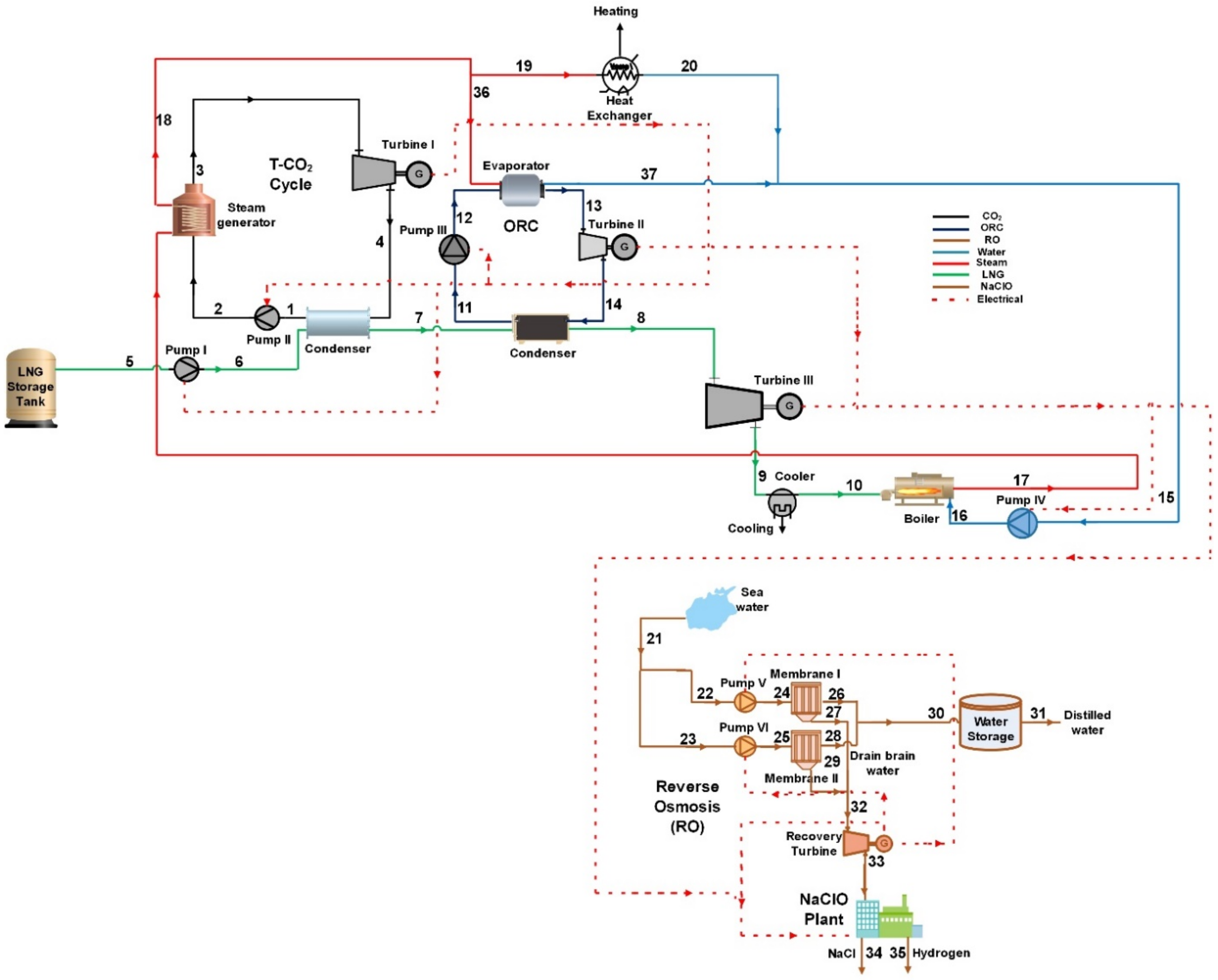
  • A new multigeneration system is proposed using LNG as a heat source and sink;
  • Energy, exergy, and economic investigations of the new configuration system are carried out;
  • Various products are generated, i.e., electrical power, heating and cooling loads, PW, hydrogen, and NaCl.

2. Materials and Methods

Figure 1 shows a schematic diagram of the cycle. The working fluids in the CO2 cycle and the organic Rankine cycle are carbon dioxide and R134a, respectively. The physical and thermodynamic properties of tetrafluoroethene (R134a) are similar to R12 with lower ozone depletion. This cycle is powered by LNG. Furthermore, the LNG is used as a heat sink. The LNG, after pressurizing in pump I (points 5, 6), absorbs the dissipated heat from the condensers of the CO2 cycle and ORC (points 6, 7, 8). Then, it is expanded in turbine III and the generator to produce electricity (points 8, 9), while it is used as a coolant fluid in the cooler (points 9, 10), where it is also converted to NG (point 10). The NG is burned in the boiler to warm the water and convert it to steam (points 16, 17). The steam provides the heat for the steam generator (CO2 cycle) and the evaporator of the ORC (points 17, 18, 36, 37). Some of the steam is used in the heater to produce heating energy (points 19, 20). The exhaust hot water of the ORC evaporator and heater is mixed, and it is transferred and pressurized in pump IV (points 15, 16, 20, 37). Some of the electricity produced in this system is consumed in the RO system to produce PW. In the RO system, seawater goes throughout pumps V and VI, and it is pressurized (points 21, 22, 23, 24, 25). The pressurized seawater is transferred to membranes I and II, and it is separated into brain water (points 27, 29) and potable water (points 26, 28, 30, 31). The brain water rotates the recovery turbine to recover energy and produce electrical power. Then, it is transferred to the NaClO plant, where it produces NaCl and hydrogen.
In the CO2 cycle, the working fluid (CO2) is pressurized in pump II (points 1, 2). Then, it exchanges energy with steam in a steam generator (points 2, 3, 17, 18), becoming superheated steam (point 3). Turbine I and the generator are operated by this superheated steam to produce electricity (points 3, 4). The turbine’s exhaust steam changes to liquid by dissipating heat to LNG (points 1, 4, 6, 7). In the ORC, the working fluid (R134a) is pressurized in pump III (points 11, 12). The pressurized working fluid exchanges heat with steam in the evaporator (points 12, 13, 36, 37). Turbine II is rotated by the superheated steam (points 13, 14). Then, the working fluid transfers heat to LNG (points 7, 8, 11, 14).
In summary, in this cycle, four components produce electricity (turbines I, II, III, and the recovery turbine), while six components (pumps I to VI) and the NaClO plant consume electricity. Figure 2 shows the energy flow between the subsystems of the proposed system.
The following assumptions are made in this study [14,21,32,33,34]:
(a)
The system works in steady-state conditions;
(b)
The ambient pressure and temperature are 288 K and 1 bar, respectively;
(c)
Pressure loss in the heat exchanger is assumed to be 2%;
(d)
The kinetic and potential energies are ignored;
(e)
The pressure loss in the cycles is ignored;
(f)
The turbine and pump polythrophic efficiencies are assumed to be 80%;
(g)
The heat exchanger effectiveness factor is assumed to be 80%;
(h)
The salt concentration in the electrolyzer is assumed constant;
(i)
The inlet CO2 and LNG of the pump are in a liquid state;
(j)
The RO recovery ratio is 0.3.

2.1. Mathematical Modeling Approach

2.1.1. Mass and Energy Balance

In general, the mass and energy balance equations are described as shown below [35].
i n m ˙ = o u t m ˙ ,  
Q ˙ W ˙ = P m ˙ ( h f + ( h h 0 ) ) R m ˙ ( h f + ( h h 0 ) ) ,  
where W ˙   and   Q ˙   are the power and heat transfer rate, while m ˙ and h are the mass flow rate and enthalpy, respectively. Subscripts R, f, P, and 0 denote reactant, formation, product, and dead state, respectively.
The mass and energy balance relationships for the CO2 cycle, ORC, LNG and water loops, and boiler are shown in Table 2 [23,36,37].
The mass balance equations in the RO system are shown below [14,38,39].
m ˙ S W = m ˙ B W + m ˙ P W ,  
m ˙ S W x S W = m ˙ P W x P W + m ˙ B w x B W ,  
where x is the salt concentration. Subscripts PW, SW, and BW denote potable water, seawater, and brain water, respectively.
The sea and potable water relationship is shown below [14,38].
m ˙ P W = R R m ˙ S W ,  
where RR denotes the recovery ratio.
The osmosis pressure for the sea, potable, and brain water streams is shown below [14,38].
π S W = R u T x S W ,  
π P W = R u T x P W ,  
π B W = R u T x B W ,  
where R defines the universal gas constant.
The membrane net pressure equation is shown below [14,38].
Δ π = ( π S W + π B W 2 ) π P W .  
The water permeability coefficient is shown below [14,38].
R W = 6.84 × 10 8 ( 18.68 0.177 x B W ) T S W .  
The RO pump net pressure is calculated as shown below [14,38].
Δ P = m ˙ P W R W A m + Δ π ,  
where A m is the membrane area.
The power consumption of the RO pump can be calculated as shown below [14,38].
W ˙ P , R O = Δ P m ˙ S W ρ S W ƞ P , R O ,  
where ρ is the density.
The mass, energy, and concentration balance relationships for the RO system are shown in the Table 3.
The following reaction can be considered in the NaClO plant:
NaCl + H2O → NaClO + H2.
In the NaClO plant, the following relationships can be considered [14,38]:
T N a C l O = T B W + 14 ,
x N a C l O = 1 6 x B W .
The NaClO plant power consumption is as follows [14,38]:
W ˙ N a C l O = 10 5 ( 5.9 × 3600 × m ˙ N a C l O × x N a C l O ) 1.05 .
The NaClO plant concentration, mass, and energy balance relationships are shown in Table 4.
The electrical power production of the system is calculated as follows:
W ˙ n e t , s y s = i = 1 3 W ˙ T , i + W ˙ r e c o v e r y   t u r b i n e i = 1 6 W ˙ P , i W ˙ N a C l O .  
The system energy efficiency is expressed as
η e n , s y s = m ˙ 31 h 31 + m ˙ 34 h 34 + m ˙ 35 h 35 + W ˙ n e t , s y s + Q ˙ h e a t e r + Q ˙ c o o l e r m ˙ 21 h 21 + m ˙ 10 L H V .  

2.1.2. Exergy Analysis

The specific exergy is expressed below, neglecting the kinetic and potential exergies [40,41].
e = x i e x c h i + ( h h 0 ) T 0 ( s s 0 ) + T 0 x i R i   ln y i ,
where x and e are the mass fractions and specific exergy, respectively, T, h, and s are the temperature, specific enthalpy, and specific entropy, respectively, and y denotes the mole fraction. Subscript ch denotes chemical. Abbreviations i and 0 represent the species and the dead state condition.
Table 5 shows the exergy destruction rates and exergy efficiencies for the system components [23,42,43].
The system exergy efficiency is expressed below.
η e x , s y s = m ˙ 31 e 31 + m ˙ 34 e 34 + m ˙ 35 e 35 + W ˙ n e t , s y s + Q ˙ h e a t e r   ( 1 T 0 T 19 ) + Q ˙ c o o l e r   ( 1 T 9 T 0 ) m ˙ 21 e 21 + m ˙ 5 e 5 .

2.1.3. Thermo-Economic Analysis

The multigeneration annual income and outcome are calculated as follows [44,45]:
C F = A p o w e r c p o w e r + A c o o l i n g c c o o l i n g + A P W c P W + A N a C l c N a C l + A H 2 c H 2 A L N G c L N G ,
where c is the specific cost, and A is the annual capacity of system production. The costs of products are shown in Table 6.
The system investment cost can be calculated as shown below [44,45].
C 0 = C O R C + C C O 2   c y c l e + C L N G   l o o p + C W a t e r   l o o p + C R O + C N a C l O   ,
where C is the investment cost of each component, as shown in Table 7. The operation and maintenance cost is assumed to be 3% of the initial cost [51,52,53,54].
In Table 7, A, H, D, and V denote the surface area, head of pump or turbine, diameter, and volume, respectively.
The logarithmic method is applied to calculate the surface area of the heat exchanger, as shown below [51].
Q ˙ = U A F t Δ T I n ,
where Q ˙ is the heat transfer rate, Δ T I n is the logarithmic mean temperature difference, A and U denote the surface area and overall heat transfer coefficient, respectively, and F is the correction factor. The overall heat transfer coefficient values for components are shown in Table 8 [52].
The effect of inflation can be seen in the following relationship [64]:
C n = C 0 ( 1 + i ) n ,
where i and n are the inflation rate (3%) and the number of years, respectively [65].
The simple payback period (SPP) can be calculated as shown below [44,45].
S P P = C n C F .
The payback period (PP) can be calculated as shown below [44,45,66].
P P = l n ( C F C F r × C n ) l n ( 1 + r ) ,
where r is the discount factor (3%).
The net present value (NPV) can be obtained as follows [44,45]:
N P V = C F ( 1 + r ) N 1 r ( 1 + r ) N C n ,
where N is the project lifetime (25 years) [44,45].
The internal rate of return (IRR) can be calculated as follows [55,67,68]:
I R R = C F C n [ 1 1 ( 1 + I R R ) N ] .

3. Results and Discussion

3.1. Simulation Method Description

For the simulation, a computer code provided in the engineering equation solver (EES) software was used. The computer code input information is shown in Table 9.

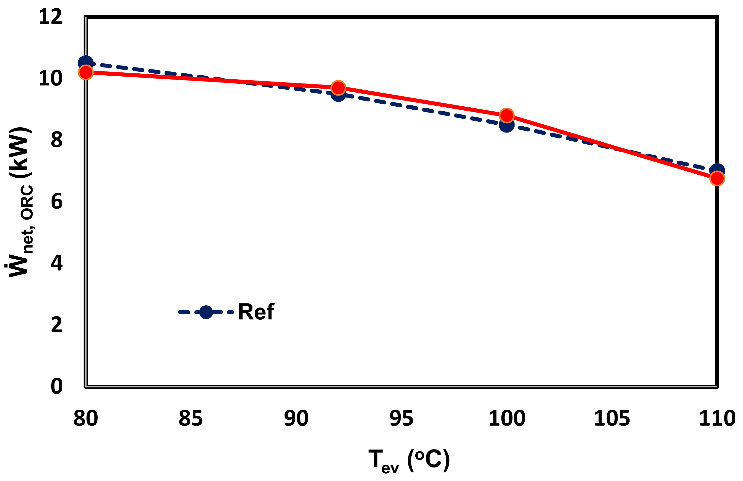
3.2. Model Validation

Since the proposed plant had a new configuration, its complete validation was not achievable. Hence, each subsystem was considered. To validate the CO2 cycle and LNG loop, the results in [32] were considered. Four key parameters (CO2 and LNG turbine power production and pump power production) were compared. Table 10 shows a comparison between the present work and the results in [32]. The source of error was related to the calculation of thermodynamic properties, which features slight differences in each software.
To validate the ORC results, Figure 2 in [56] was considered. R600a was selected as the working fluid. The data for the ORC presented in [56] were used. Figure 3 shows a comparison between the net output power of this work and the results in [56]. The maximum error was 3.5%, which is compatible with engineering calculations. The source of error was similar to that of the CO2 cycle.
For RO validation, the results in [14] were used. Table 11 shows the comparison. The error ranged from 0.7% to 7% due to some information about membrane performance not being exactly clarified in [14] For NaClO plant validation, the results in [57] were used. The electrical power consumption of the NaClO plant was found to be 4 kW, while this value was theoretically calculated as 3.78 kW by the computer code. The error of 5.5% was related to the type and model of the NaClO plant.

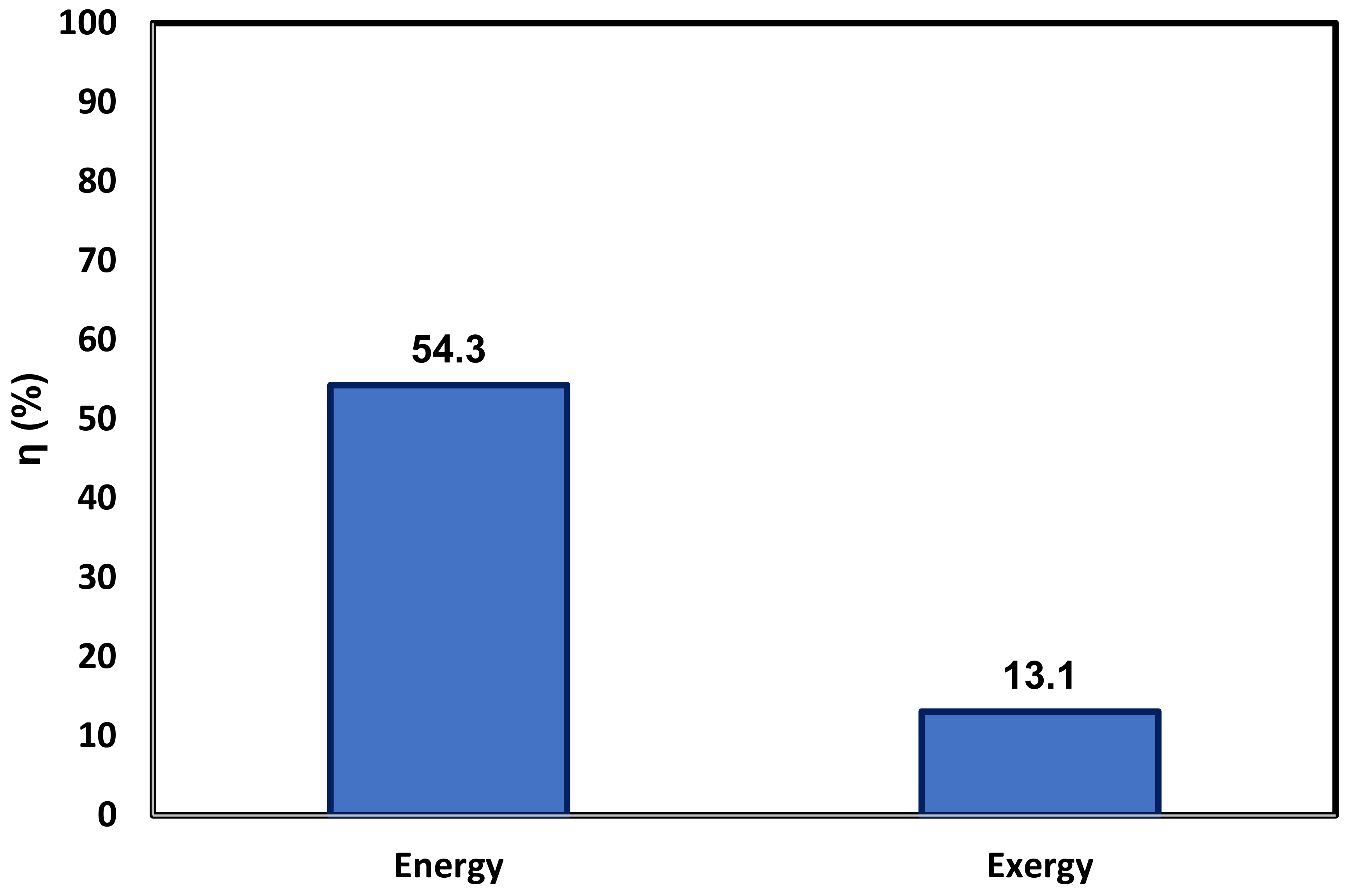
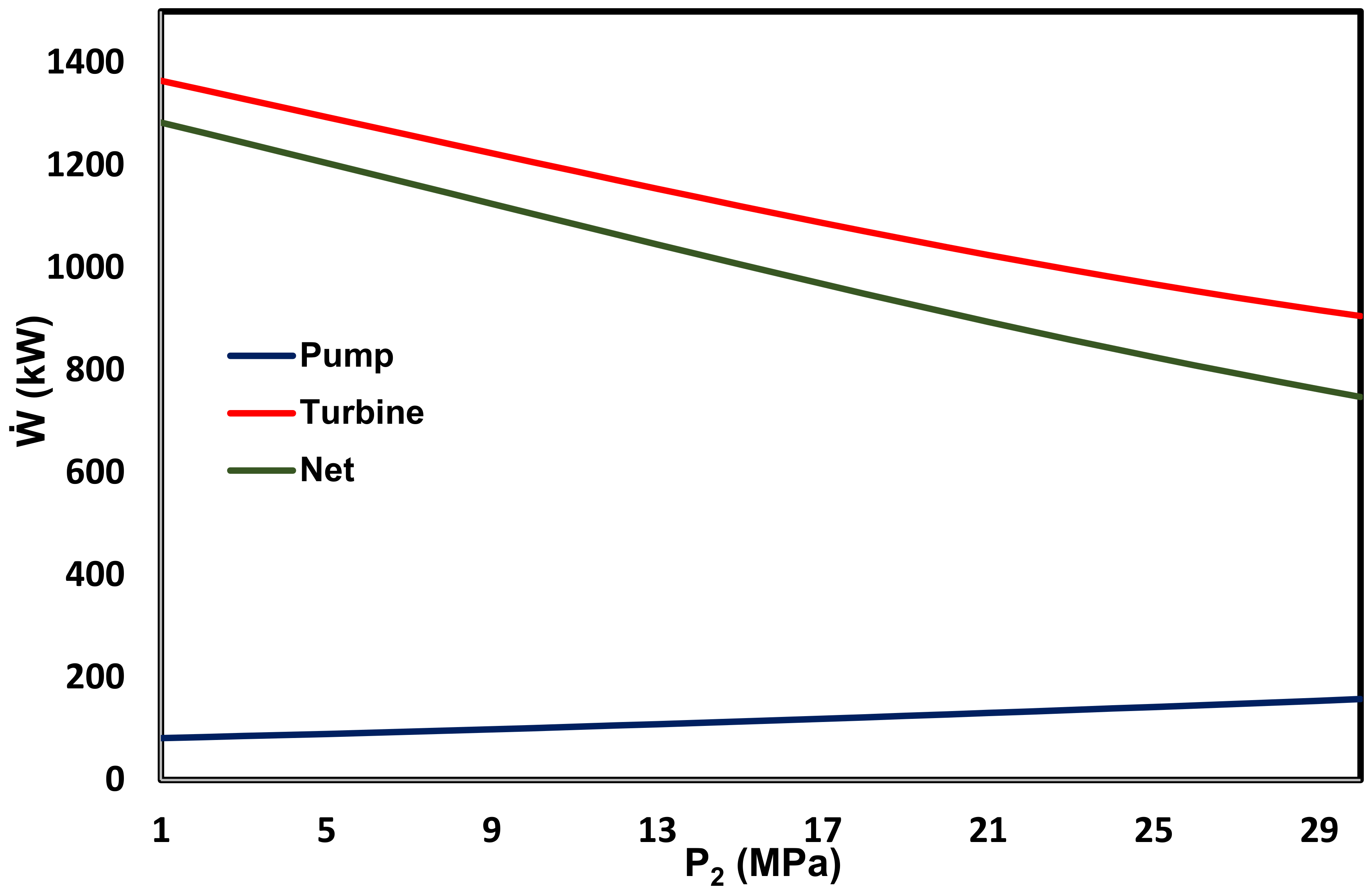
3.3. Energy and Exergy Analyses

Table 12 shows the thermodynamic properties at every point of the system. Table 13 shows the values of the system products. This system produces 10.53 GWh of electrical energy, 276.4 GWh of cooling energy, 1783 GWh of heating energy, 17,280 m3 of potable water, 739.56 tons of hydrogen, and 383.78 tons of salt in a year. The ratios of cooling and heating energies to electrical energy are 26.25 and 169.33, respectively. Figure 4 shows the system energy and exergy efficiencies. According to the figure, the energy and exergy efficiencies are 54.3% and 13.1%, respectively. The system energy efficiency is much higher than the system exergy efficiency, as, in the exergy efficiency equation (Equation (20)), both the heat and the cooling production rates are multiplied by the ratios, which are lower than the unit. The variation in RO and NaClO plant power consumption and in recovery turbine and system power productions versus seawater inlet mass flow rate (21) is shown in Figure 5. Upon increasing the ṁ21 from 1 to 5 kg/s, the power consumption of the RO and NaClO plant can be increased from 1.486 and 134.8 kW to 35.7 and 673.9 kW, respectively. According to the equations presented in Table 3, the power consumption of the RO pumps has a linear relationship with the mass flow rate of feed water. According to Equation (16), the power consumption of the NaClO plant also has a linear relationship with feed brain water.
The net electrical power production of the total proposed system is reduced from 1456.7 kW to 876.7 kW following this increase in 21.
The system energy and exergy efficiencies versus seawater mass flow rate (21) are shown in Figure 6. Increasing the seawater mass flow rate did not have a major effect on the system energy and exergy efficiencies. Upon increasing the seawater mass flow rate from 1 to 5 kg/s, the system energy and exergy efficiencies were reduced from 54.25% and 13.11% to 54.23% and 13.01%, respectively. It can be concluded that the system energy and exergy efficiencies remained constant. Since the extra electrical power consumed by the NaClO and RO systems is compensated for by the extra energy and exergy flows of PW, NaCl, and hydrogen, according to Equations (18) and (20).
Figure 7 shows the changes in pump electrical power consumption and turbine electrical power production, as well as the net output power of the CO2 cycle, with the variation in outlet pressure of the pump (P2) in the CO2 cycle. Upon increasing the outlet pressure of the pump, the electrical power consumption of the pump in the CO2 cycle is increased. Moreover, the electrical power production of the turbine is decreased. This is because the superheat temperature at point 3 is fixed at 493.1 K (above the supercritical temperature), which is about 293.1 K less than the superheated steam temperature at point 17 according to pinch analysis.
Thus, by increasing the outlet pressure of the pump in the CO2 cycle (P2) at a fixed temperature (493.1 K), the enthalpy at point 3 is reduced, and the electrical power production in the turbine is reduced. It is clear that, by increasing the electrical power consumption of the pump and the electrical power production of the turbine, the net electrical power of the CO2 cycle is decreased.
Figure 8 shows the variation in CO2 cycle energy and exergy efficiencies with outlet pump pressure in the CO2 cycle. According to Figure 7, the CO2 cycle net output electrical power is reduced upon increasing the outlet pressure of the pump, whereas the inlet heat rate of the CO2 cycle ( (h17–h18)) remains constant.
The change in net output power of the ORC with pump outlet pressure at different inlet turbine temperatures is shown in Figure 9. Upon increasing the ORC pump outlet pressure, the cycle net output power is reduced, since it decreases the enthalpy value at point 13. Furthermore, the power consumption of the pump increases. Upon increasing the turbine inlet temperature in the ORC, the net output electrical power is increased by increasing the enthalpy at point 13.
The contribution to exergy destruction rate of each subsystem is presented in Figure 10. The highest contribution comes from the water loop, which includes a heater, burner/boiler, and pump IV. In the burner, a chemical reaction (combustion) warms the water in the boiler, thereby converting water to steam. Thus, this loop has the highest exergy destruction rate. In distant second place, the CO2 cycle has a considerable exergy destruction rate due to the heat transfer taking place in the steam generator and condenser. The lowest exergy destruction rate occurs in the RO system, as the pressures and temperatures in this system are all close to the dead state.

3.4. Thermo-Economic Analyses

Table 14 shows the key economic parameters for the system. The system’s NPV is 908.9 million USD, the system’s PP and SPP are equal to 7.9 and 6.9 years, and the system’s IRR is 0.138.
Figure 11 shows the variation in PP and SPP versus feed seawater mass flow rate. Upon increasing the seawater mass flow rate, both PP and SPP are reduced, which is beneficial. Specifically, upon increasing the feed seawater mass flow rate from 1 kg/s to 5 kg/s, the PP is reduced from 8.7 to 6.2 years and the SPP is reduced from 7.56 to 5.59 years.
In general, increasing the seawater mass flow causes the following effects:
(a)
Increase in the initial cost of the NaClO and RO plants (negative effect);
(b)
Increase in the system product costs (NaCl, PW, and hydrogen) due to an increase in these products;
(c)
Decrease in the electrical power product cost due to an increase in RO and NaClO plant power consumption.
The magnitude of the second effect exceeds that of the other two effects; thus, both PP and SPP are reduced upon increasing the feed seawater mass flow rate.
The variation in system NPV with the mass flow rate of seawater is depicted in Figure 12. The NPV of the system is increased upon increasing the mass flow rate of seawater. Similar to Figure 11, it is clear that, if more electrical power is consumed to produce PW, NaCl, and hydrogen, it is more beneficial.

4. Conclusions

A new integrated system was proposed in this paper which simultaneously uses LNG as a heat source and sink. Through this method, the ratio of the heat sink and source temperatures is high, thereby improving system performance.
The CO2 cycle and ORC are combined to generate electricity in this proposed system. In both cycles, LNG is used to absorb the heat dissipated by condensers, as well as to produce cooling load. Subsequently, the LNG is converted to NG. The NG is used to convert water into steam in the burner and boiler, thus meeting the energy needs of the steam generator and evaporator in the CO2 cycle and the ORC, in addition to producing heating load. A portion of the electrical power generated in the two mentioned cycles is used to produce hydrogen, salt, and PW in the RO and NaClO plants. The main conclusions are summarized below.
(a)
In comparison with a system featuring LNG only as a heat sink [14], which uses solar energy through a flat plate collector as the heat source, the system energy and exergy efficiencies are further improved from 12.4% and 4.45% to 54% and 13.1%, respectively.
(b)
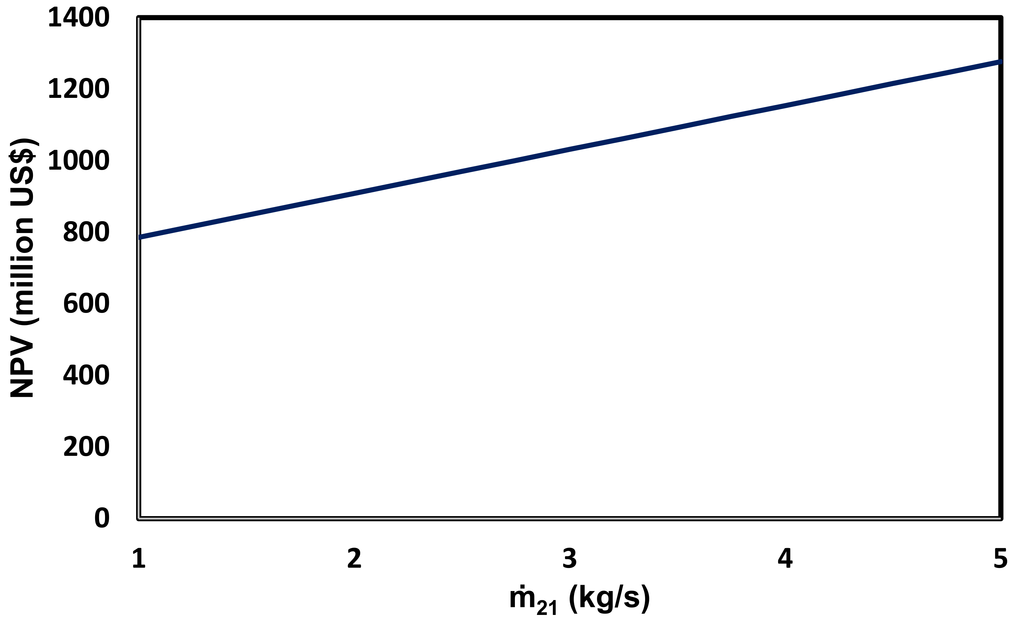
The NPV of this system is equal to 908.9 million USD.
(c)
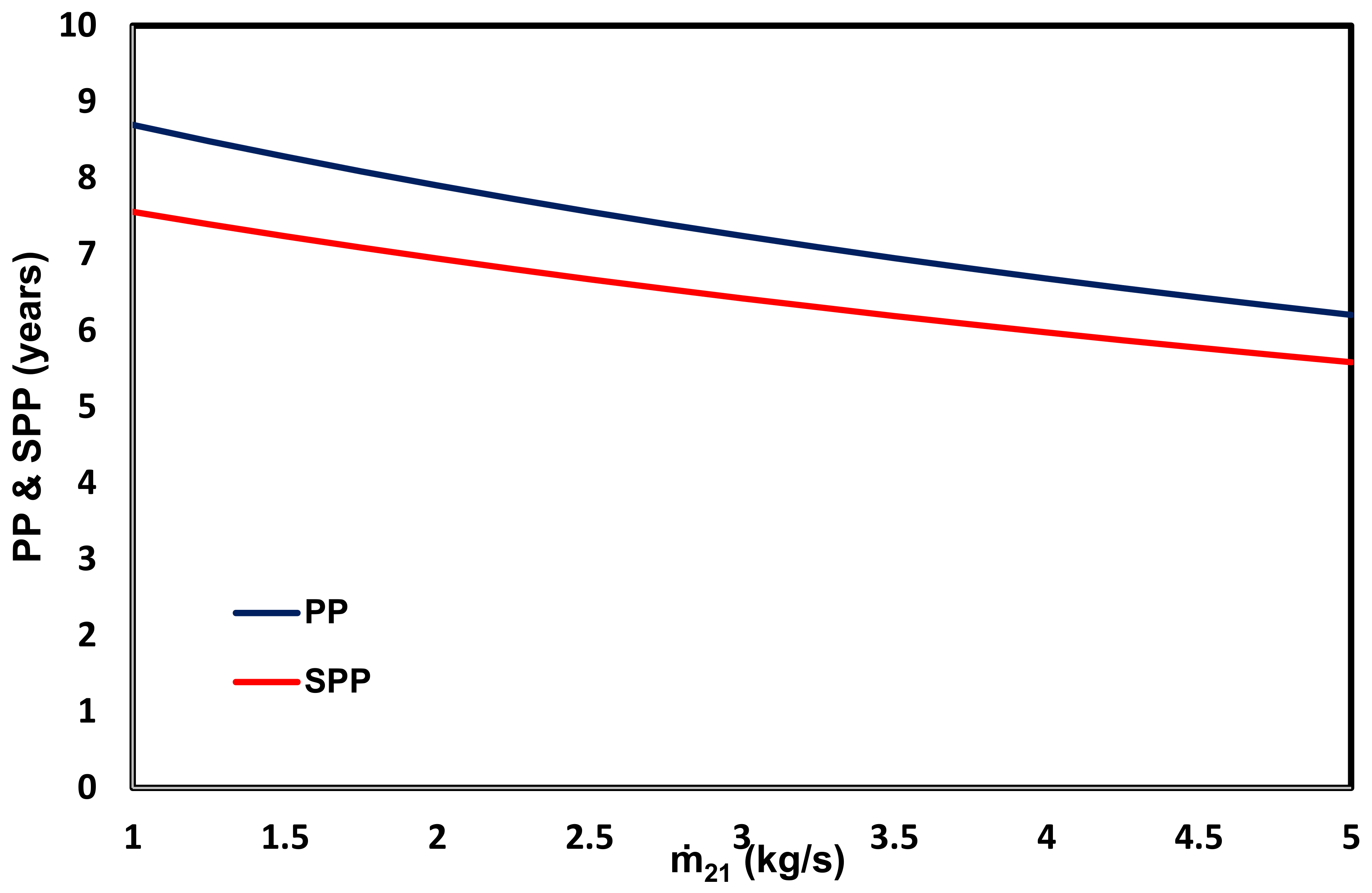
The PP and SPP of this system are 7.9 and 6.9 years, respectively.
(d)
The IRR value of this system is equal to 0.138.
(e)
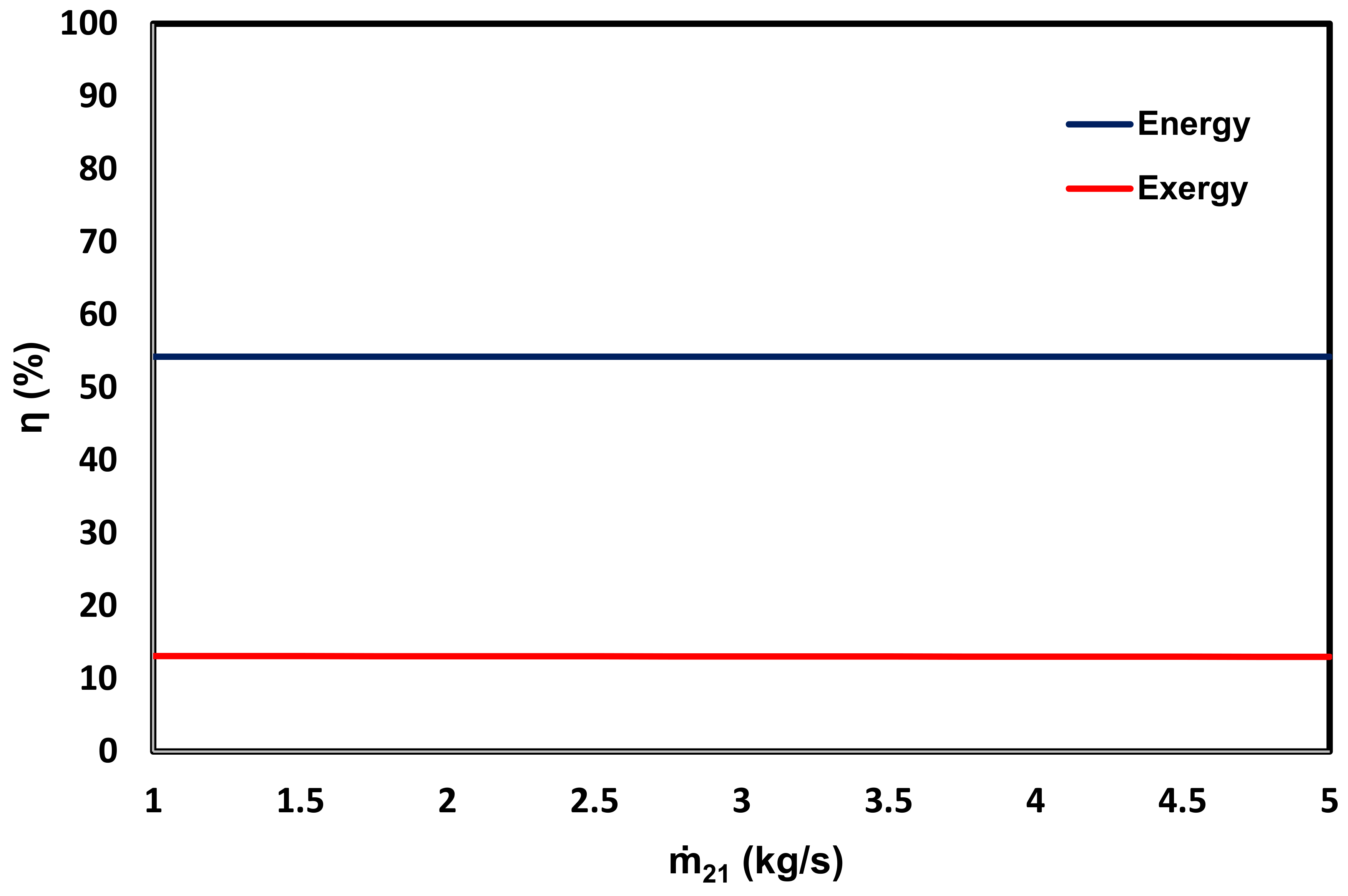
Greater desalination of seawater to produce PW, salt, and hydrogen is beneficial according to the economic evaluation.
(f)
Greater seawater desalination does not have a considerable effect on the system energy and exergy efficiencies.
(g)
The highest and lowest contributions to the exergy destruction rates were presented by the water loop and RO system.
In the future, the integration of various cycles such as the Kalina and Goswami cycles can be examined as alternatives.

Author Contributions

Conceptualization, T.T., M.A.E. and A.A.; methodology, T.T. and M.A.E.; software, T.T. and M.A.E.; validation, M.A.E., A.A. and S.H.; formal analysis, T.T., M.A.E. and A.A.; investigation, M.A.E. and A.A.; resources, T.T. and M.A.E.; data curation, M.A.E.; writing—original draft preparation, M.A.E., A.A. and S.H.; writing—review and editing, S.M., S.H., M.A.E. and A.A.; visualization, T.T., M.A.E., S.M., S.H. and A.A.; project administration, T.T., M.A.E., A.A., S.H. and S.M.; funding acquisition, M.A.E., A.A., S.H. and S.M. All authors have read and agreed to the published version of the manuscript.

Funding

This research received no external funding.

Institutional Review Board Statement

Not Applicable.

Informed Consent Statement

Not Applicable.

Data Availability Statement

Not applicable.

Acknowledgments

The authors would like to express their appreciation for the financial and scientific assistance provided by Hasan Barzegar and Ali Rajaei from the Energy Optimization Research and Development Group (EORD), Tehran, Iran.

Conflicts of Interest

The authors declare no conflict of interest.

Nomenclature

Symbols (units)Description
A (m2)Area
C 0 (USD)System investment cost
C n (USD)System investment cost in a specific year
CF (USD)Multigeneration annual income
e (kJ/kg)Specific exergy
Ė   kW Exergy rate
Ft (-)Correction factor
g (m/s2)Gravitational acceleration
h (kJ/kg)Specific enthalpy
c (USD/kWh)Product-specific cost
C (USD)Investment cost
RW (1/K)Water permeability coefficient
m ˙ (kg/s)Mass flow rate
N (years)Project lifetime
P (kPa)Pressure
Q ˙ (kW)Heat transfer rate
r (-)Discount factor
R (kJ/kmoleK)Global gas constant
s (kJ/kgK)Specific entropy
TTemperature
U (W/m2K)Overall heat transfer coefficient
V (m3)Volume
W ˙ (kW)Power
x (-)Mass fraction, concentration of salt
y (-)Mole fraction
Y (USD/kWh, USD/kg)Annual capacity of system production
Greek SymbolsDescription
η (-)Polythrophic efficiency
Δ π (Pa)Net pressure membrane
AbbreviationsDescription (Units)
IRRInternal rate of return (-)
NPVNet present value (USD)
PPPayback period (-)
RRRecovery ratio (years)
SPPSimple payback period (kW)

References

  1. Omoregie, U. After the Crash: Oil Price Recovery and LNG Project Viability. Nat. Resour. 2019, 10, 179–186. [Google Scholar] [CrossRef] [Green Version]
  2. Ehyaei, M.; Ahmadi, A.; Assad, M.E.H.; Rosen, M.A. Investigation of an integrated system combining an Organic Rankine Cycle and absorption chiller driven by geothermal energy: Energy, exergy, and economic analyses and optimization. J. Clean. Prod. 2020, 258, 120780. [Google Scholar] [CrossRef]
  3. Kumar, S.; Kwon, H.-T.; Choi, K.-H.; Lim, W.; Cho, J.H.; Tak, K.; Moon, I. LNG: An eco-friendly cryogenic fuel for sustainable development. Appl. Energy 2011, 88, 4264–4273. [Google Scholar] [CrossRef]
  4. Chen, Y.; He, L.; Guan, Y.; Lu, H.; Li, J. Life cycle assessment of greenhouse gas emissions and water-energy optimization for shale gas supply chain planning based on multi-level approach: Case study in Barnett, Marcellus, Fayetteville, and Haynesville shales. Energy Convers. Manag. 2017, 134, 382–398. [Google Scholar] [CrossRef]
  5. Lv, Q.; Liu, H.; Wang, J.; Liu, H.; Shang, Y. Multiscale analysis on spatiotemporal dynamics of energy consumption CO2 emissions in China: Utilizing the integrated of DMSP-OLS and NPP-VIIRS nighttime light datasets. Sci. Total. Environ. 2020, 703, 134394. [Google Scholar] [CrossRef]
  6. Uwitonze, H.; Han, S.; Jangryeok, C.; Hwang, K.S. Design process of LNG heavy hydrocarbons fractionation: Low LNG temperature recovery. Chem. Eng. Process. Process. Intensif. 2014, 85, 187–195. [Google Scholar] [CrossRef]
  7. Nakaiwa, M.; Akiya, T.; Owa, M.; Tanaka, Y. Evaluation of an energy supply system with air separation. Energy Convers. Manag. 1996, 37, 295–301. [Google Scholar] [CrossRef]
  8. Messineo, A.; Panno, G. LNG cold energy use in agro-food industry: A case study in Sicily. J. Nat. Gas Sci. Eng. 2011, 3, 356–363. [Google Scholar] [CrossRef]
  9. Wang, P.; Chung, T.-S. A conceptual demonstration of freeze desalination–membrane distillation (FD–MD) hybrid desalination process utilizing liquefied natural gas (LNG) cold energy. Water Res. 2012, 46, 4037–4052. [Google Scholar] [CrossRef] [PubMed]
  10. Jansen, S.; Woudstra, N. Understanding the exergy of cold: Theory and practical examples. Int. J. Exergy 2010, 7, 693–713. [Google Scholar] [CrossRef] [Green Version]
  11. Liu, E.; Lv, L.; Yi, Y.; Xie, P. Research on the Steady Operation Optimization Model of Natural Gas Pipeline Considering the Combined Operation of Air Coolers and Compressors. IEEE Access 2019, 7, 83251–83265. [Google Scholar] [CrossRef]
  12. Otsuka, T. Evolution of an LNG terminal: Senboku Terminal of Osaka gas. In Proceedings of the 23rd World Gas Conference, Amsterdam, The Netherlands, 5–9 June 2006; pp. 2617–2630. [Google Scholar]
  13. Li, Z.-G.; Cheng, H.; Gu, T.-Y. Research on dynamic relationship between natural gas consumption and economic growth in China. Struct. Chang. Econ. Dyn. 2019, 49, 334–339. [Google Scholar] [CrossRef]
  14. Naseri, A.; Bidi, M.; Ahmadi, M.H. Thermodynamic and exergy analysis of a hydrogen and permeate water production process by a solar-driven transcritical CO2 power cycle with liquefied natural gas heat sink. Renew. Energy 2017, 113, 1215–1228. [Google Scholar] [CrossRef]
  15. Qi, M.; Park, J.; Kim, J.; Lee, I.; Moon, I. Advanced integration of LNG regasification power plant with liquid air energy storage: Enhancements in flexibility, safety, and power generation. Appl. Energy 2020, 269, 115049. [Google Scholar] [CrossRef]
  16. Franco, A.; Casarosa, C. Thermodynamic analysis of direct expansion configurations for electricity production by LNG cold energy recovery. Appl. Therm. Eng. 2015, 78, 649–657. [Google Scholar] [CrossRef]
  17. Yu, H.; Kim, D.; Gundersen, T. A study of working fluids for Organic Rankine Cycles (ORCs) operating across and below ambient temperature to utilize Liquefied Natural Gas (LNG) cold energy. Energy 2019, 167, 730–739. [Google Scholar] [CrossRef]
  18. Ahmadi, A.; El Haj Assad, M.; Jamali, D.; Kumar, R.; Li, Z.; Salameh, T.; Al-Shabi, M.; Ehyaei, M. Applications of geothermal organic Rankine Cycle for electricity production. J. Clean. Prod. 2020, 274, 122950. [Google Scholar] [CrossRef]
  19. Ghaebi, H.; Namin, A.S.; Rostamzadeh, H. Exergoeconomic optimization of a novel cascade Kalina/Kalina cycle using geothermal heat source and LNG cold energy recovery. J. Clean. Prod. 2018, 189, 279–296. [Google Scholar] [CrossRef]
  20. Angelino, G.; Invernizzi, C.M. The role of real gas Brayton cycles for the use of liquid natural gas physical exergy. Appl. Therm. Eng. 2011, 31, 827–833. [Google Scholar] [CrossRef]
  21. Ahmadi, A.; Jamali, D.; Ehyaei, M.; Assad, M.E.H. Energy, exergy, economic and exergoenvironmental analyses of gas and air bottoming cycles for production of electricity and hydrogen with gas reformer. J. Clean. Prod. 2020, 259, 120915. [Google Scholar] [CrossRef]
  22. Pattanayak, L.; Padhi, B.N. Thermodynamic analysis of combined cycle power plant using regasification cold energy from LNG terminal. Energy 2018, 164, 1–9. [Google Scholar] [CrossRef]
  23. Ahmadi, M.H.; Mehrpooya, M.; Pourfayaz, F. Exergoeconomic analysis and multi objective optimization of performance of a Carbon dioxide power cycle driven by geothermal energy with liquefied natural gas as its heat sink. Energy Convers. Manag. 2016, 119, 422–434. [Google Scholar] [CrossRef]
  24. Xue, X.; Guo, C.; Du, X.; Yang, L.; Yang, Y. Thermodynamic analysis and optimization of a two-stage organic Rankine cycle for liquefied natural gas cryogenic exergy recovery. Energy 2015, 83, 778–787. [Google Scholar] [CrossRef]
  25. Xu, J.; Lin, W. A CO2 cryogenic capture system for flue gas of an LNG-fired power plant. Int. J. Hydrog. Energy 2017, 42, 18674–18680. [Google Scholar] [CrossRef]
  26. Stradioto, D.A.; Seelig, M.F.; Schneider, P.S. Reprint of: Performance analysis of a CCGT power plant integrated to a LNG regasification process. J. Nat. Gas Sci. Eng. 2015, 27, 18–22. [Google Scholar] [CrossRef]
  27. Shi, X.; Agnew, B.; Che, D.; Gao, J. Performance enhancement of conventional combined cycle power plant by inlet air cooling, inter-cooling and LNG cold energy utilization. Appl. Therm. Eng. 2010, 30, 2003–2010. [Google Scholar] [CrossRef]
  28. Atienza-Márquez, A.; Bruno, J.C.; Akisawa, A.; Coronas, A. Performance analysis of a combined cold and power (CCP) system with exergy recovery from LNG-regasification. Energy 2019, 183, 448–461. [Google Scholar] [CrossRef]
  29. Ayou, D.S.; Eveloy, V. Energy, exergy and exergoeconomic analysis of an ultra low-grade heat-driven ammonia-water combined absorption power-cooling cycle for district space cooling, sub-zero refrigeration, power and LNG regasification. Energy Convers. Manag. 2020, 213, 112790. [Google Scholar] [CrossRef]
  30. Taheri, M.; Mosaffa, A.; Farshi, L.G. Energy, exergy and economic assessments of a novel integrated biomass based multigeneration energy system with hydrogen production and LNG regasification cycle. Energy 2017, 125, 162–177. [Google Scholar] [CrossRef]
  31. Liu, Y.; Han, J.; You, H. Performance analysis of a CCHP system based on SOFC/GT/CO2 cycle and ORC with LNG cold energy utilization. Int. J. Hydrog. Energy 2019, 44, 29700–29710. [Google Scholar] [CrossRef]
  32. Naseri, A.; Bidi, M.; Ahmadi, M.H.; Saidur, R. Exergy analysis of a hydrogen and water production process by a solar-driven transcritical CO 2 power cycle with Stirling engine. J. Clean. Prod. 2017, 158, 165–181. [Google Scholar] [CrossRef] [Green Version]
  33. Ferrero García, R.; Carbia Carril, J.; Romero Gomez, J.; Romero Gomez, M. Power plant based on three series Rankine cycles combined with a direct expander using LNG cold as heat sink. Energy Convers. Manag. 2015, 101, 285–294. [Google Scholar] [CrossRef]
  34. Pan, Z.; Zhang, L.; Zhang, Z.; Shang, L.; Chen, S. Thermodynamic analysis of KCS/ORC integrated power generation system with LNG cold energy exploitation and CO2 capture. J. Nat. Gas Sci. Eng. 2017, 46, 188–198. [Google Scholar] [CrossRef]
  35. Xia, W.; Huo, Y.; Song, Y.; Han, J.; Dai, Y. Off-design analysis of a CO2 Rankine cycle for the recovery of LNG cold energy with ambient air as heat source. Energy Convers. Manag. 2019, 183, 116–125. [Google Scholar] [CrossRef]
  36. Behzadi, A.; Gholamian, E.; Ahmadi, P.; Habibollahzade, A.; Ashjaee, M. Energy, exergy and exergoeconomic (3E) analyses and multi-objective optimization of a solar and geothermal based integrated energy system. Appl. Therm. Eng. 2018, 143, 1011–1022. [Google Scholar] [CrossRef]
  37. Ghasemian, E.; Ehyaei, M.A. Evaluation and optimization of organic Rankine cycle (ORC) with algorithms NSGA-II, MOPSO, and MOEA for eight coolant fluids. Int. J. Energy Environ. Eng. 2017, 9, 39–57. [Google Scholar] [CrossRef] [Green Version]
  38. Bejan, A. Advanced Engineering Thermodynamics; John Wiley & Sons: Hoboken, NJ, USA, 2016. [Google Scholar]
  39. Li, Z.; Ehyaei, M.; Kamran Kasmaei, H.; Ahmadi, A.; Costa, V. Thermodynamic modeling of a novel solar powered quad generation system to meet electrical and thermal loads of residential building and syngas production. Energy Convers. Manag. 2019, 199, 111982. [Google Scholar] [CrossRef]
  40. Talebizadehsardari, P.; Ehyaei, M.; Ahmadi, A.; Jamali, D.; Shirmohammadi, R.; Eyvazian, A.; Ghasemi, A.; Rosen, M.A. Energy, exergy, economic, exergoeconomic, and exergoenvironmental (5E) analyses of a triple cycle with carbon capture. J. CO2 Util. 2020, 41, 101258. [Google Scholar] [CrossRef]
  41. Yargholi, R.; Kariman, H.; Hoseinzadeh, S.; Bidi, M.; Naseri, A. Modeling and advanced exergy analysis of integrated reverse osmosis desalination with geothermal energy. Water Sci. Technol. Water Supply 2020, 20, 984–996. [Google Scholar] [CrossRef]
  42. El-Dessouky, H.T.; Ettouney, H.M. Fundamentals of Salt Water Desalination; Elsevier: Amsterdam, The Netherlands, 2002. [Google Scholar]
  43. Lazzaretto, A.; Tsatsaronis, G. SPECO: A systematic and general methodology for calculating efficiencies and costs in thermal systems. Energy 2006, 31, 1257–1289. [Google Scholar] [CrossRef]
  44. Bejan, A.; Tsatsaronis, G.; Moran, M. Thermal Design and Optimization; John Wiley and Sons, Inc.: New York, NY, USA, 1996. [Google Scholar]
  45. Ehyaei, M.A.; Ahmadi, A.; Rosen, M.A.; Davarpanah, A. Thermodynamic Optimization of a Geothermal Power Plant with a Genetic Algorithm in Two Stages. Processes 2020, 8, 1277. [Google Scholar] [CrossRef]
  46. Zeinodini, M.; Aliehyaei, M. Energy, exergy, and economic analysis of a new triple-cycle power generation configuration and selection of the optimal working fluid. Mech. Ind. 2019, 20, 501. [Google Scholar] [CrossRef] [Green Version]
  47. Bellos, E.; Pavlovic, S.; Stefanovic, V.; Tzivanidis, C.; Nakomcic-Smaradgakis, B.B. Parametric analysis and yearly performance of a trigeneration system driven by solar-dish collectors. Int. J. Energy Res. 2019, 43, 1534–1546. [Google Scholar] [CrossRef]
  48. Tzivanidis, C.; Bellos, E.; Antonopoulos, K.A. Energetic and financial investigation of a stand-alone solar-thermal Organic Rankine Cycle power plant. Energy Convers. Manag. 2016, 126, 421–433. [Google Scholar] [CrossRef]
  49. Nami, H.; Ertesvåg, I.S.; Agromayor, R.; Riboldi, L.; Nord, L.O. Gas turbine exhaust gas heat recovery by organic Rankine cycles (ORC) for offshore combined heat and power applications—Energy and exergy analysis. Energy 2018, 165, 1060–1071. [Google Scholar] [CrossRef]
  50. Ehyaei, M.; Ahmadi, A.; Rosen, M.A. Energy, exergy, economic and advanced and extended exergy analyses of a wind turbine. Energy Convers. Manag. 2019, 183, 369–381. [Google Scholar] [CrossRef]
  51. Alizadeh, S.M.; Ghazanfari, A.; Ehyaei, M.A.; Ahmadi, A.; Jamali, D.H.; Nedaei, N.; Davarpanah, A. Investigation the Integration of Heliostat Solar Receiver to Gas and Combined Cycles by Energy, Exergy, and Economic Point of Views. Appl. Sci. 2020, 10, 5307. [Google Scholar] [CrossRef]
  52. Flinnsci. Sodium Chloride Laboratory Grade 500 g. 2020. Available online: https://www.flinnsci.com/sodium-chloride-laboratory-grade-500-g/s0063/ (accessed on 3 June 2020).
  53. Nami, H.; Akrami, E. Analysis of a gas turbine based hybrid system by utilizing energy, exergy and exergoeconomic methodologies for steam, power and hydrogen production. Energy Convers. Manag. 2017, 143, 326–337. [Google Scholar] [CrossRef]
  54. Lee, H.-J.; Yoo, S.-H.; Huh, S.-Y. Economic benefits of introducing LNG-fuelled ships for imported flour in South Korea. Transp. Res. Part D Transp. Environ. 2020, 78, 102220. [Google Scholar] [CrossRef]
  55. Lecompte, S.; Huisseune, H.; Broek, M.V.D.; De Schampheleire, S.; De Paepe, M. Part load based thermo-economic optimization of the Organic Rankine Cycle (ORC) applied to a combined heat and power (CHP) system. Appl. Energy 2013, 111, 871–881. [Google Scholar] [CrossRef]
  56. Alshammari, F.; Karvountzis-Kontakiotis, A.; Pesyridis, A.; Usman, M. Expander Technologies for Automotive Engine Organic Rankine Cycle Applications. Energies 2018, 11, 1905. [Google Scholar] [CrossRef] [Green Version]
  57. Bejan, A.; Tsatsaronis, G.; Moran, M.J. Thermal Design and Optimization; John Wiley & Sons: Hoboken, NJ, USA, 1995. [Google Scholar]
  58. Couper, J.R.; Penney, W.R.; Fair, J.R.; Walas, S.M. (Eds.) Chapter 21—Costs of Individual Equipment. In Chemical Process Equipment, 2nd ed.; Gulf Professional Publishing: Burlington, VT, USA, 2005; pp. 719–728. [Google Scholar]
  59. Roosen, P.; Uhlenbruck, S.; Lucas, K. Pareto optimization of a combined cycle power system as a decision support tool for trading off investment vs. operating costs. Int. J. Therm. Sci. 2003, 42, 553–560. [Google Scholar] [CrossRef]
  60. Yuanda Henan China. 1000 kg/H Steam Boiler Natural Gas/LPG/CNG/LNG Fired Steam Boiler with High Quality—China Steam Boiler, Gas Fired Steam Boiler. Available online: https://yuandaboiler.en.made-in-china.com/product/oXqEAynPZOcI/China-1000kg-H-Steam-Boiler-Natural-Gas-LPG-CNG-LNG-Fired-Steam-Boiler-with-High-Quality.html (accessed on 15 June 2020).
  61. Du, Y.; Xie, L.; Liu, J.; Wang, Y.; Xu, Y.; Wang, S. Multi-objective optimization of reverse osmosis networks by lexicographic optimization and augmented epsilon constraint method. Desalination 2014, 333, 66–81. [Google Scholar] [CrossRef]
  62. Ahmadi, A.; Esmaeilion, F.; Esmaeilion, A.; Ehyaei, M.A.; Silveira, J.L. Benefits and Limitations of Waste-to-Energy Conversion in Iran. Renew. Energy Res. Appl. 2020, 1, 27–45. [Google Scholar] [CrossRef]
  63. Marques, R.C. Comparing private and public performance of Portuguese water services. Hydrol. Res. 2007, 10, 25–42. [Google Scholar] [CrossRef]
  64. Pierobon, L.; Nguyen, T.-V.; Larsen, U.; Haglind, F.; Elmegaard, B. Multi-objective optimization of organic Rankine cycles for waste heat recovery: Application in an offshore platform. Energy 2013, 58, 538–549. [Google Scholar] [CrossRef] [Green Version]
  65. Berhane, H.G.; Gonzalo, G.G.; Laureano, J.; Dieter, B. Design of environmentally conscious absorption cooling systems via multi-objective optimization and life cycle assessment. Appl. Energy 2009, 86, 1712–1722. [Google Scholar] [CrossRef]
  66. Shafer, T. Calculating Inflation Factors for Cost Estimates. In City of Lincoln Transportation and Utilities Project Delivery; Public Works: Lincoln, NE, USA, 2021. [Google Scholar]
  67. Alaloul, W.S.; Musarat, M.A.; Liew, M.; Qureshi, A.H.; Maqsoom, A. Investigating the impact of inflation on labour wages in Construction Industry of Malaysia. Ain Shams Eng. J. 2021. [Google Scholar] [CrossRef]
  68. Edalati, S.; Ameri, M.; Iranmanesh, M.; Tarmahi, H.; Gholampour, M. Technical and economic assessments of grid-connected photovoltaic power plants: Iran case study. Energy 2016, 114, 923–934. [Google Scholar] [CrossRef]
  69. Emara, H.I. Nutrient salts, inorganic and organic carbon contents in the waters of the Persian Gulf and the Gulf of Oman. J. Persian Gulf 2010, 1, 33–44. [Google Scholar]
  70. FILMTEC™ Membranes. How to Evaluate the Active Membrane Area of Seawater Reverse Osmosis Elements. 2015. Available online: dupont.com/content/dam/dupont/amer/us/en/water-solutions/public/documents/en/45-D01504-en.pdf (accessed on 3 June 2020).
Figure 1. Schematic diagram of the system.
Energies 14 02849 g001
Figure 2. Energy flow between the subsystems.
Energies 14 02849 g002
Figure 3. Comparison of the net output power in the present work with that in [14] versus the evaporator temperature of the ORC.
Energies 14 02849 g003
Figure 4. The system energy and exergy efficiencies.
Energies 14 02849 g004
Figure 5. The variation in RO, NaClO plant, recovery turbine, and system power with inlet seawater mass flow rate (21).
Energies 14 02849 g005
Figure 6. The system energy and exergy efficiencies versus seawater mass flow rate (21).
Energies 14 02849 g006
Figure 7. The changes in pump and turbine electrical power consumption/production and net output power of the CO2 cycle with the variation in pump outlet pressure (P2) in the CO2 cycle.
Energies 14 02849 g007
Figure 8. The variation in CO2 cycle energy and exergy efficiencies with outlet pump pressure in the CO2 cycle.
Energies 14 02849 g008
Figure 9. The variation in net output power of the ORC with pump outlet pressure at different inlet turbine temperatures.
Energies 14 02849 g009
Figure 10. Contributions of each system to the exergy destruction rate.
Energies 14 02849 g010
Figure 11. The variation in PP and SPP versus feed seawater mass flow rate.
Energies 14 02849 g011
Figure 12. The variation in system NPV with the feed seawater mass flow rate.
Energies 14 02849 g012
Table 1. Studies related to multigeneration systems.
No. Energy ResourceLNGComponentsProductsResultsRef
Heat SourceHeat
Sink
1Solar CO2 cycle, FPC, RO, NaClO plant, Stirling engineElectrical, NaCl, hydrogen, PWThe exergy destruction rate was decreased from 16.7% to 8.8% upon replacement of the condenser by a Stirling engine[32]
2Solar Transcritical CO2 cycle, FPC, RO, NaClO plantElectrical, NaCl, hydrogen, PWThe system net output power was increased by increasing the inlet temperature of the boiler and turbine
3Geothermal CO2 cycleElectricalThe system exergy efficiency was equal to 20.5%
The product cost rate was equal to 263,592.15 USD/year
[14]
4Exhaust hot gas
of combined cycle
Two-stage ORCElectricalThe energy and exergy efficiencies were 25.64% and 31.02%
CPP was equal to 6.3 USD/W
5LNG RC, ASU, LAESElectrical, clean airThe maximum amount of net output power ranged from 85.7–94.8 kJ/kg LNG[23]
6LNG ASU, GC, CO2 captureElectrical, CO290% CO2 recovery
7NG RC, direct expanderElectricalThe maximum exergy efficiency was obtained by 302.8 kJ/kg LNG[24]
8LNGCCGT, LNG regasification processElectricalThe electrical efficiency was increased from 6.32% to 9.09%
9LNGCCPP, IAC, intercoolingElectricalThe electrical efficiency was improved by 2.8%[15]
10LNGCCPPElectricalThis system produced 3.36 MW and 21 MW of electrical power and cooling
11Geothermal Absorption power/cooling cycleElectricalThe system energy and exergy efficiencies were equal to 39% and 36%, respectively[25]
12Biomass ARS, GC, RC, ORC, PEM ElecElectrical, cooling, and hydrogenUpon increasing the fuel mass flow rate from 4 to 10 kg/s, the system energy efficiency decreased by 8.5% and the cost rate increased by 122.8%
13LNGSOFC, GC, CO2 cycle, ORC, CO2 captureElectrical, cooling, heating, and CO2The system exergy efficiency was equal to 62.3%[33]
14Exhaust gas KC, ORC, CO2 captureElectrical, CO2The system energy efficiency was equal to 36%
The system exergy efficiency was equal to 41.4%
The net electrical power output was equal to 394,658 kW
15Ambient air CO2 Rankine cycleElectricalThe system thermal efficiency was equal to 6.75%
The net output power was 108.7 kW
[26]
Table 2. Mass and energy balance relationships for the CO2 cycle, ORC, LNG and water loops, and boiler.
No.ComponentsMass BalanceEnergy Equation
CO2 cycle
1Pump II (P) m ˙ 1 = m ˙ 2 w ˙ p I I = m ˙ 1 ( h 2 h 1 )
2Steam generator m ˙ 2 = m ˙ 3 ,   m ˙ 17 = m ˙ 18   m ˙ 2 ( h 3 h 2 ) = η H X m ˙ 17 ( h 17 h 18 )
3Turbine I (T) m ˙ 3 = m ˙ 4 w ˙ T I = m ˙ 3 ( h 3 h 4 )
4Condenser m ˙ 4 = m ˙ 1 ,   m ˙ 6 = m ˙ 7 m ˙ 7 ( h 7 h 6 ) η H X = m ˙ 1 ( h 4 h 1 )
ORC
5Pump III (P) m ˙ 11 = m ˙ 12 w ˙ p I I I = m ˙ 1 ( h 2 h 1 )
6Steam generator m ˙ 12 = m ˙ 13 ,   m ˙ 36 = m ˙ 37   m ˙ 12 ( h 13 h 12 ) = η H X m ˙ 36 ( h 36 h 37 )
7Turbine II (T) m ˙ 13 = m ˙ 14 w ˙ T I I = m ˙ 13 ( h 13 h 14 )
8Condenser m ˙ 14 = m ˙ 11 ,   m ˙ 7 = m ˙ 8 m ˙ 7 ( h 8 h 7 ) η H X = m ˙ 11 ( h 14 h 11 )
LNG loop
9Pump I (P) m ˙ 5 = m ˙ 6 w ˙ p I = m ˙ 5 ( h 6 h 5 )
10Turbine III (T) m ˙ 8 = m ˙ 9 w ˙ T I I I = m ˙ 8 ( h 8 h 9 )
11Cooler m ˙ 9 = m ˙ 10 Q ˙ c o o l e r = η H X m ˙ 9 ( h 10 h 9 )
Boiler
12Boiler m ˙ 17 = m ˙ 18 η C C m ˙ 10 L H V = m ˙ 16 ( h 17 h 16 )
Water loop
13Pump IV (P) m ˙ 15 = m ˙ 16 w ˙ p I V = m ˙ 15 ( h 16 h 15 )
14Heater m ˙ 19 = m ˙ 20 Q ˙ h e a t e r = η H X m ˙ 19 ( h 19 h 20 )
Table 3. Mass, energy, and concentration balance relationships for the RO system.
No.ComponentsMass BalanceEnergy Equationx
1Pump V m ˙ 22 = m ˙ 24 W ˙ P V = m ˙ 22 ( h 24 h 22 ) x 24 = x 22
2Pump VI m ˙ 23 = m ˙ 25 W ˙ P I V = m ˙ 23 ( h 25 h 23 ) x 23 = x 25
3Membrane I m ˙ 24 = m ˙ 26 + m ˙ 27 m ˙ 24 h 24 = m ˙ 26 h 26 + m ˙ 27 h 27 m ˙ 24 x 24 = m ˙ 26 x 26 + m ˙ 27 x 27
4Membrane II m ˙ 25 = m ˙ 28 + m ˙ 29 m ˙ 25 h 25 = m ˙ 28 h 28 + m ˙ 29 h 29 m ˙ 25 x 25 = m ˙ 28 x 28 + m ˙ 29 x 29
5Recovery turbine m ˙ 32 = m ˙ 33 W ˙ R e c o v e r y   t u r b i n e = m ˙ 32 ( h 32 h 33 ) x 32 = x 33
Table 4. Mass, energy, and concentration balance relationships for the NaClO plant.
Mass Balance m ˙ 38 = m ˙ 34 + m ˙ 35
Concentration Balance m ˙ 38 x 38 = m ˙ 34 x 34 + m ˙ 35 x 35
Energy Balance m ˙ 38 h 38 + W ˙ N a C l O = m ˙ 34 h 34 + m ˙ 35 h 35
Table 5. The exergy destruction rates and exergy efficiencies for system components.
No.ComponentsExergy EfficiencyExergy Destruction Rate (kW)
CO2 cycle
1Pump II (P) W ˙ P I I m ˙ 1 ( e 2 e 1 ) m ˙ 1 e 1 m ˙ 2 e 2 + W ˙ P I I
2Steam generator m ˙ 2 ( e 3 e 2 ) m ˙ 17 ( e 17 e 18 ) m ˙ 2 e 2 +   m ˙ 3 e 3 + m ˙ 17 e 17 m ˙ 18 e 18
3Turbine I (T) W ˙ T I m ˙ 3 ( e 3 e 4 ) m ˙ 3 e 3 m ˙ 4 e 4 W ˙ T I
4Condenser m ˙ 1 ( e 4 e 1 ) m ˙ 6 ( e 7 e 6 ) m ˙ 4 e 4 m ˙ 1 e 1 + m ˙ 6 e 6 m ˙ 7 e 7
ORC
5Pump III (P) W ˙ P I I I m ˙ 1 ( e 12 e 11 ) m ˙ 11 e 11 m ˙ 12 e 12 + W ˙ P I I I
6Evaporator m ˙ 12 ( e 13 e 12 ) m ˙ 17 ( e 36 e 37 ) m ˙ 12 e 12 m ˙ 13 e 13 + m ˙ 36 e 36 m ˙ 37 e 37
7Turbine II (T) W ˙ T I I m ˙ 13 ( e 13 e 14 ) m ˙ 13 e 13 m ˙ 14 e 14 W ˙ T I I I
8Condenser m ˙ 1 ( e 14 e 11 ) m ˙ 6 ( e 8 e 7 ) m ˙ 14 e 14 m ˙ 11 e 11 + m ˙ 7 e 7 m ˙ 8 e 8
LNG loop
9Pump I (P) W ˙ P I m ˙ 5 ( e 6 e 5 ) m ˙ 5 e 5 m ˙ 6 e 6 + W ˙ P I
10Turbine III (T) W ˙ T I I I m ˙ 13 ( e 8 e 9 ) m ˙ 8 e 8 m ˙ 9 e 9 W ˙ T I I I
11Cooler Q ˙ c o o l e r   ( 1 T 9 T 0 ) m ˙ 9 ( e 10 e 9 ) m ˙ 9 e 9 m ˙ 10 e 10 Q ˙ c o o l e r   ( 1 T 9 T 0 )
Boiler
12Boiler m ˙ 16 ( e 17 e 16 ) m ˙ 10 e 10 m ˙ 16 e 16 m ˙ 17 e 17 + m ˙ 10 e 10
Water loop
13Pump IV (P) W ˙ P I V m ˙ 15 ( e 16 e 15 ) m ˙ 15 e 15 m ˙ 16 e 16 + W ˙ P I V
14Heater Q ˙ h e a t e r   ( 1 T 0 T 19 ) m ˙ 19 ( e 19 e 20 ) m ˙ 19 e 19 m ˙ 20 e 20 Q ˙ h e a t e r   ( 1 T 0 T 19 )
RO
15Pump V W ˙ P V m ˙ 22 ( e 24 e 22 ) m ˙ 22 ( e 22 e 24 ) + W ˙ P V
16Pump VI W ˙ P V I m ˙ 23 ( e 25 e 23 ) m ˙ 23 ( e 23 e 25 ) + W ˙ P V I
17Membrane I m ˙ 26 e 26 m ˙ 24 e 24 m ˙ 24 e 24 m ˙ 27 e 27 m ˙ 26 e 26
18Membrane II m ˙ 28 e 28 m ˙ 25 e 25 m ˙ 25 e 25 m ˙ 29 e 29 m ˙ 28 e 28
19Recovery turbine W ˙ r e c o v e r y   t u r b i n e m ˙ 32 ( e 32 e 33 ) m ˙ 32 e 32 m ˙ 33 e 33 W ˙ r e c o v e r y   t u r b i n e
NaClO
20NaClO plant m ˙ 34 e 34 + m ˙ 35 e 35 W ˙ N a C l O m ˙ 38 e 38 + W ˙ N a C l O m ˙ 35 e 35 m ˙ 34 e 34
Table 6. The specific costs of fuel and products.
Specific Cost Value Ref
cpower0.21 USD/kWh[46]
cPW0.0004 USD/kg[47]
ccooling/cheating0.07 USD/kWh[48]
cNaCl10.47 USD/kg[49]
cH213.96 USD/kg[50]
cLNG0.025 USD/kWh[48]
Table 7. Values of investment and installation costs for different components.
No.ComponentsCost FunctionRef
CO2 cycle
1Pump 10 3.3892 + 0.05361 l o g W + 0.1538 ( l o g W ) ˙ 2 ˙ [23]
2Steam generator   ( A / 0.093 ) 0.78 [23]
3Turbine 10 2.6259 + 1.43981 l o g W 0.1776 ( l o g W ) ˙ 2 ˙ [23]
4Condenser   ( A / 0.093 ) 0.78 [23]
ORC
5Pump 1026 × ( W ˙ / 300 ) ˙ 0.25 [55]
6Evaporator 216.6 + 353.4 × A [55]
7Turbine 2237 × W ˙ 0.41 [56]
8Condenser 338.6 × A [55]
LNG loop
9LNG turbine 479.34   ( m ˙ 8 0.93 η T ) ln ( P 8 P 9 ) ( 1 exp ( 0.036 T 8 54.4 ) ) [57]
10LNG pump 3 × exp ( 8.833 0.6019 ln ( Q ˙ H ) + 0.06019 ( ln ( Q ˙ H ) ) 2 ) [58]
11LNG cooler 1.218 × exp ( 0.4692 + 0.1203 ln ( Q ˙ ) + 0.0931 ( ln ( Q ˙ ) ) 2 ) [58]
Water loop
12Pump 3540 × W ˙ 0.71 [59]
13Boiler33,600,000[60]
14Heater η h e a t e r 1.218 × f d × f p × c b
f d =   exp ( 1.1156 + 0.0906 × ln(10.76A))
f p =   0.7771 + 0.04981 × ln(10.76A)
c b = exp (   8.821 0.30863 ×   ln   ( 10.76 A ) + 0.0681 × ln (10.76A)
×   ln   ( 10.76 A ) )
[58]
RO
15Pump 996 × ( 864.00 × Q ) ˙ 0.8 [61]
16Membrane50[62]
17Storage Tank 1.14 × ( 158.62 × V T a n k + 18 , 321 ) [63]
18Recovery turbine 52 × ( 864.00 × Q ˙ × Δ P 0.8 ) [61]
NaClO
19NaClO (HD:6000)45,000[14]
Table 8. The overall heat transfer coefficient values for components.
No.Components U   ( W m 2 K )
2Boiler500
3Heat exchanger700
4Condenser800
Table 9. Input information of the simulation code.
ParameterUnitValueRef
m ˙ 1 kg/s6.73[41]
T1K220[41]
T2K224.9[41]
T3K493.1[41]
P1kPa600[41]
P2kPa12,490[41]
x21mg/L40,200[69]
x30mg/L150[69]
Amm235.3[70]
RR-0.3[14]
21kg/s2-
Table 10. The comparison of key parameters in the present work and in [32].
No.ParameterUnitPresent WorkRef [32]Error (%)
1 W ˙ T , C O 2 kW14.214.663.1
2 W ˙ P , C O 2 kW4.984.7784.2
3 W ˙ T , L N G kW7.197.4643.6
4 W ˙ P , L N G kW3.813.6933.1
Table 11. Validation results of the RO system.
No.ParameterModelRef [14]Error (%)
10 m ˙ b r a i n ( kg s ) 1.0921.1040.7
2 m ˙ b r a i n ( kg s ) 0.4680.4562.6
3 m ˙ b r a i n ( kg s ) 3.453.7117
4 m ˙ b r a i n ( kg s ) 8.428.966
Table 12. The thermodynamic properties at every point of the system.
NoT (K)P (kPa) (kg/s)X (-)h (kJ/kg)e (kJ/kg)
1220.06006.73-−420210.7
2224.912,4906.73-−407.2220.1
3493.212,4906.73-141288.3
4220.56106.73-−74.91104.7
5111.5101.49.547-−911.71015
6115.365809.547-−8891019
7210.564409.547-−372.5655.8
8283.263109.547-−104.5599.4
9255.340009.547-−148.7542.9
10288.240009.547-−4672548.9
11271.928010.26-50.1835.22
12295.3709.110.26-89.4535.27
13403.2709.110.26-369.260.63
14272.928010.26-249.723.31
15303.2101.3115.5-125.81.579
16303.2150115.5-125.81.627
17513.2150115.5-2952705
18493.2150115.5-2912687.9
19493.2150114.3-2912687.9
20303.2101.3114.3-125.81.579
21288.2101.3240,02059.4513.46
22288.2101.3140,02059.4513.46
23288.2101.3140,02059.4513.46
24288.24767140,02063.6917.98
25288.24767140,02063.6917.98
26288.247670.315067.494.659
27288.247670.757,10761.836.596
28288.247670.315067.494.659
29288.247670.757,10761.836.596
30288.247670.615067.494.659
31288.2101.30.615063.050.000242
32288.247671.457,10761.836.596
33288.2303.91.457,10757.842.323
34507.2101.30.01333-205.9156.5
35298.2101.30.02568-78851226
36493.21501.288-2912687.9
37303.2101.31.288-125.81.579
38288.2101.314-57.842.323
Table 13. The values of system products.
ProductUnitValue
Wnet,systemGWh/year12.75
QcoolingGWh/year276.4
QheatingGWh/year1783
VPWm3/year17,280
mNaClTon/year383.76
mH2Ton/year739.56
Table 14. The key economic parameters for the system.
No.ParameterUnitValue
1NPVmillion USD908.9
2PPyears7.9
3SPPyears6.9
4IRR-0.138
Publisher’s Note: MDPI stays neutral with regard to jurisdictional claims in published maps and institutional affiliations.

