Abstract
A new hybrid meta-heuristic approach Jaya–PPS, which is the combination of the Jaya algorithm and Powell’s Pattern Search method, is proposed in this paper to solve the optimal power flow (OPF) problem for minimization of fuel cost, emission and real power losses and total voltage deviation simultaneously. The recently developed Jaya algorithm has been applied for the exploration of search space, while the excellent local search capability of the PPS (Powell’s Pattern Search) method has been used for exploitation purposes. Integration of the local search procedure into the classical Jaya algorithm was carried out in three different ways, which resulted in three versions, namely, J-PPS1, J-PPS2 and J-PPS3. These three versions of the proposed hybrid Jaya–PPS approach were developed and implemented to solve the OPF problem in the standard IEEE 30-bus and IEEE 57-bus systems integrated with distributed generating units optimizing four objective functions simultaneously and IEEE 118-bus system for fuel cost minimization. The obtained results of the three versions are compared to the Dragonfly Algorithm, Grey Wolf Optimization Algorithm, Jaya Algorithm and already published results using other methods. A comparison of the results clearly demonstrates the superiority of the proposed J–PPS3 algorithm over different algorithms/versions and the reported methods.
1. Introduction
With the increasing trend of penetration of renewable distributed generating (DG) units in the present day inter-connected restructured power system, the importance of solving optimal power flow problems has increased many folds. Optimal power flow results are crucial for planning, economic operation and control of an existing electrical power system, as well as for its future expansion planning. At the beginning of the 1960s, Carpentier addressed the OPF problem as an extension of economic load dispatch for the first time in history [1]. Since then, researchers have contributed significantly to this crucial issue. In a given electrical network, the OPF solution is required to regulate the control or decision variables set in the feasible region that optimizes some pre-defined objective functions. For the OPF problem, the control variables used are: Vg (generator bus voltages), Pg (generators’ active power outputs excluding slack bus), phase shifters, Tr (tap-settings of regulating transformer) and Qc (injected reactive power using capacitor banks, FACTS devices etc.). Some of these variables are discrete, e.g., Tr, injected reactive power source output Qc, phase shifters, while others are continuous (e.g., Pg and Vg). The discrete nature of the control variable poses a challenge for the optimization technique and makes OPF a non-convex problem [2,3].
Integration of DGs seems to be quite appealing, but it is important to analyze their impact in a power network [4]. Optimal location and size of the DG unit have a significant effect on the reliability of power supply, operational cost, voltage profile, power loss and environmental pollution and voltage stability in a power system. Therefore, it has become a crucial task for researchers and industry personnel to determine the optimal location for DG and the size of the DG [5]. With the increase of the power injection from DGs into a power network, it is equally important to find out the optimum power generation and optimal setting of other control parameters to minimize fuel cost, emission cost and real power loss with an improved voltage profile [6].
OPF is a complex optimization problem, which associates several constraints and decision or control variables. The common objectives of the OPF problem are fuel cost minimization, emission minimization, real power loss minimization, voltage profile improvement and/or a combination of two or more of these objectives. The conventional algorithms depend on convexity to find the global best solution and are required to simplify relationships to achieve convexity. However, since the OPF problem is non-convex in general, several local minima can exist. If the valve point loading effects of thermal generators are taken into account, the non-convexity increases even further. Furthermore, traditional optimization approaches often use initial starting points (except for linear programming and convex optimization) and often converge or diverge to locally optimal solutions. These approaches are normally limited to particular cases of OPF and do not have much flexibility in terms of different kinds of objective functions or constraints that could be employed [7,8]. Except for linear programming and convex optimization, most of the conventional optimization algorithms cannot be guaranteed to be globally optimal because traditional algorithms are mainly local search. As a result, the final solution is always often dependent on the initial starting points.
Nowadays, several meta-heuristic algorithms have been developed by researchers, which are found to be powerful tools for handling difficult optimization problems. These random search, population-based algorithms are highly flexible, which means that they are appropriate to solve various types of optimization problems, including linear problems, non-linear problems and complex constrained optimization problems. Some of these methods are League Championship Algorithm (LCA) [3], Firefly Algorithm (FFA), Krill Herd Method (KH), Hybrid Firefly and Krill Herd Method (HFA) [9], Neighborhood Knowledge-based Evolutionary Algorithm (NKHA), Bare-Bones Multi-Objective Particle Swarm Optimization (BB-MOPSO), Multi-Objective Imperialist Competitive Algorithm (MOICA), Modified Non-dominated Sorting Genetic Algorithm (MNSGA-II), Multi-Objective Modified Imperialist Competitive Algorithm (MOMICA) [10], Moth Swarm Algorithm (MSA) [11], Multi-objective Evolutionary Algorithm based on decomposition-superiority of feasible (MOEA/D-SF) [12] and many others.
Recently, various hybrid algorithms have been investigated for effectively solving various optimization problems. Alsumait et al. [13] presented a hybrid GA–PS–SQP-based optimization algorithm to solve the economic dispatch (ELD) problem. Attaviriyanupap et al. [14] suggested a hybrid optimization technique based on Evolutionary Programming and SQP algorithms for dynamic ELD problems. An integrated predator–prey (PP) optimization and a Powell search method were both proposed for the multi-objective hydrothermal scheduling problem [15]. Mahdad et al. [16] applied a hybrid DE-APSO-PS strategy to solve multi-objective power system planning. A hybrid modified imperialist competitive algorithm and SQP were employed to handle the constrained OPF problem [17]. Recently, considerable attention has been given to the Deep Neural Network approaches to the Energy Management problem [18,19].
It is observed that all Evolutionary Computing (EC)-based algorithms have some advantages and some disadvantages. Two main parts of any EC-based algorithm are exploration and exploitation. Some algorithms have good exploration capability but poor exploitation and vice versa. The recently developed Jaya algorithm is capable of exploration, while Powell’s Pattern Search (PPS) method has good search space exploitation capability. Hence, to boost the operational proficiency of the Jaya algorithm, Powell’s Pattern Search method has been incorporated into it. Proper inclusion of the advantages of the Jaya and PPS algorithm would lead to better results for real-world complex, constrained and high-dimensional optimization problems. In the proposed hybrid Jaya–PPS algorithm, the Jaya algorithm was applied to explore a search space that is likely to provide the near-global solution and subsequently, the PPS algorithm was applied to attain a better solution.
The paper’s contribution can be summed up as follows:
- The main contribution of this paper is to implement hybridization of two algorithms (Jaya and Powell’s Pattern Search) in different manners and at different levels to find the best option for hybridization.
- Powell’s Pattern Search method has been incorporated into the Jaya algorithm in three different ways, resulting in three variants, namely, J-PPS1, J-PPS2 and J-PPS3.
- The proposed hybrid Jaya and Powell’s Pattern Search method utilizes the exploration property of the Jaya algorithm and the exploitation quality of Powell’s Pattern Search method.
- This paper handles the OPF problem considering DG with four objectives functions simultaneously, namely, minimization of fuel cost, emission, real power losses and voltage profile improvement by converting the multi-objective OPF into a single objective OPF.
- In addition to Dragonfly Algorithm (DA), Grey Wolf Optimization (GWO) and Classical Jaya algorithms, three versions of hybrid Jaya and PPS, J-PPS1, J-PPS2 and J–PPS3 for the OPF problem are developed, wherein the excellent search capability of the PPS method has been exploited for further improvement of the solution provided by Jaya algorithm.
2. Problem Formulation
Mathematically, the objective function together and operating constraints of the OPF problem considered in this work are as follows [20]:
Subject to the constraints given by Equation (2).
where M (W,X) is the objective function to be minimized, g (W,X) and h (W,X) are the equality and inequality constraints, respectively.
The control variables () include: the generator active power output () except at slack bus, generator bus voltage (), tap-setting of transformer () and shunt VAR compensation (). The dependent variables () consists of slack bus active power output , Load bus voltage (), generator reactive power output () and power flow in transmission lines (). The control variables and state variables vectors can be expressed by Equation (3):
A control or decision variable can have any value within its minimum and maximum limits. In actual practice, transformer tap settings are not continuous variables. However, in this paper, to compare the results with the reported results, all the decision variables are considered to be continuous.
2.1. OPF Objective Functions
This paper handles the OPF problem considering DG with four objectives functions simultaneously, namely, minimization of fuel cost, emission, real power losses and improvement of voltage profile by converting the multi-objective OPF into a single objective OPF.
2.1.1. Fuel Cost Minimization
The prime motive of this objective function is to minimize the total cost of generation/fuel. It can therefore be expressed by Equation (4):
where , and are the quadratic fuel cost coefficients of the ith generating unit and is the active power output of ith generating unit.
2.1.2. Emission Cost Minimization
The total emission pollutants such as (sulfur oxides) and (nitrogen oxides), which is an approximate combination of a quadratic and an exponential function can be expressed by Equation (5)
where are the emission coefficients of ith generating unit.
2.1.3. Real Power Losses Minimization
The aim of the present case is to minimize real power losses. The total real power losses can be computed using Equation (6):
where NB is the no. of buses, is the active power generation at ith generating unit and is the real power load at ith load bus.
2.1.4. Voltage Profile Improvement
Voltage profile improvement means the voltage magnitude at load buses must not deviate much from 1.0 pu. Thus, the main motive, in this case, is to minimize voltage variation from 1.0 pu at all the load buses. In the present case, the objective function can be represented by Equation (7):
where is the voltage magnitude at ith load bus.
2.2. Constraints
The equality constraints are a combination of active and reactive non-linear power flow equations. In Equation (2), g (W,X) is a set of equality constraints and is described by Equation (8):
where NB is the no. of buses, , are the active and reactive power outputs of generating unit, are the active and reactive power outputs of DG unit, , are active and reactive power load demand and are the total active and reactive power losses occurring in the lines, respectively.
The inequality constraints h (W,X) represents operating limits of various equipment in a power system, which are described by Equation (9):
where active power output bus voltage , and reactive power output , should be regulated by their lower and upper limits for all the generators, including slack bus generator and controllable VAR sources (), Transformer taps-setting () voltage of load buses and power flow in transmission lines () should vary between their minimum and maximum limits.
2.3. Combined Objective Function (COF)
The multi-objective function, which consists of four contradictory objective functions, i.e., minimization of fuel cost, emission cost, real power loss and total voltage deviation, is transformed into a single-objective function by using weighing factors to combine the four objective functions as given below.
where , are weighing factors [9].
2.4. Incorporation of Constraints
The constraints are included in the combined objective function in the form of inequalities to find a feasible solution, and thus, the extended objective function can be defined by Equation (11):
3. Jaya Algorithm
The Jaya algorithm is a comparatively new meta-heuristic optimization algorithm developed by Rao [21]. The working principle of the Jaya algorithm is that the numerical solution that has been obtained should go towards the better solution and should avoid the inferior solutions for a particular optimization problem. The main advantage of the Jaya algorithm is that no algorithm-specific parameters are required, and thus, it is simple to implement this algorithm for solving various kinds of optimization problems.
Maximized (or minimized) value of objective function M(z)
Within the lower and upper bounds of the control variables, the initial solution p is randomly selected. After that, all the variables will be eventually updated according to Equation (12). On the basis of the fitness value of the objective function, the best and worst solutions are determined [21].
Let ‘m’ be the number of design variables (i.e., j = 1, 2, 3, …, m) and the ‘n’ is the number of candidate solutions (i.e., population size, k = 1, …, n). If represents the value of jth variable for the kth candidate in ith iteration; that value is updated according to Equation (12).
In (12), and are the best candidate and worst candidate value of variable j, respectively. The updated value of is and throughout the ith iteration, and are two random numbers for the jth variable within [0, 1].
3.1. Powell’s Pattern Search (PPS)
In 1962, Powell proposed the Powell search method, which was the expansion of the basic Pattern Search method. It is based on the conjugate direction method. Powell’s Pattern Search (PPS) method is a derivative-free optimization technique that is ideal for solving a number of optimization problems beyond the scope of conventional optimization procedures. In general, the advantage of PPS is that the structure of the algorithm is remarkably simple, easy to implement and computationally efficient as well. PPS with meta-heuristic algorithm offers a flexible, balanced operator to enhance local search capability in contrast to another meta-heuristic algorithm. The following is the summary of the PPS algorithm underlying mechanisms [15,22]:
The search direction for lth coordinate for gth dimension of the n dimension search space can be defined as:
The step length for gth decision variable can be determined as:
where, is the minimum and maximum step length for gth decision variable, respectively.
The vector of the decision variable is updated once in the direction of the coordinate (l) as:
The vector of control variables is modified on the basis of the minimum objective function value. For all ‘n’ coordinates, this process continues. The pattern search direction is obtained for the next optimization cycle:
where is the initial value of the decision variable .
Additionally, one of the coordinate’s direction was discarded in the direction of pattern ‘m’ as:
The process goes on until the entire direction of the coordinate is discarded and the entire operations restart in one of the coordinate directions again. Finally, until the Powell method has reached maximum iterations, the process of updating continues.
3.2. Proposed Hybrid Jaya–PPS Algorithm
Jaya algorithm has a strong capacity to exploit search space globally, but sometimes it suffers from premature convergence and can be stuck simply in local optima [6]. In order to overcome this problem and to make this algorithm more efficient, a hybrid Jaya algorithm, which combines the Jaya algorithm and PPS algorithm, is proposed in this paper. The PPS algorithm is a class of direct search methods. In general, it has immunity to strong local extremist trapping when used for local optimization. The proposed hybrid approach is primarily concerned with balancing the exploration and exploitation steps of the optimization procedure. PPS technique has good search space exploitation capability, while Jaya is able to explore the search space very well. The goal of incorporating PPS with Jaya is to combine the benefits of both algorithms.
Similar to other local search algorithms, the PPS algorithm is also sensitive to the initial or starting point. In selecting the initial point arbitrarily, it requires a large number of function evolutions, computation burden and slow convergence rate. In this research paper, to overcome these demerits of the PPS algorithm, the integration of local search procedure (Powell’s Pattern Search) into the classical Jaya algorithm has been carried out in three different ways and the variants of hybrid Jaya–PPS thus developed are termed as J-PPS1, J-PPS2 and J-PPS3. To evaluate the performances of these variants, the common controlling parameters and the total number of function evaluations (NFE) used in J-PPS1, J-PPS2 and J-PPS3 algorithms are set the same as the classical Jaya algorithm. As stated, all the hybrid algorithms have the same number of function evaluations; thus, the additional criterion introduced in the proposed hybrid algorithms is to maintain (balance) the total number of function evaluations. The NFE has been used as a reference to the check efficiency of various algorithms in this paper.
In the first strategy (J-PPS1), the PPS algorithm was applied considering its initial point as the solution offered by the Jaya algorithm after applying it for 25% iterations. In this case, the optimization process is a two-step process. In step 1 (first 25% of Itermax), the Jaya algorithm was applied. However, in step 2 (remaining 75% of iterations), the PPS algorithms were applied using the optimal setting of control variables offered by the Jaya algorithm as initial point setting.
In the second strategy (J-PPS2), the Jaya algorithm and PPS algorithm were applied for an equal number of iterations to maintain the balance between the exploration and exploitation capability of the proposed J-PPS2 algorithm. In other words, the optimization process was completed in two steps. In step 1 (50% of Itermax), the Jaya algorithm was applied, while in step 2 (for the remaining 50% iterations), the PPS algorithms were applied sequentially as in the case of J-PPS1.
In the third strategy (J-PPS3), the PPS algorithm was applied after exploiting the 75% problem-solving capability of the Jaya algorithm, i.e., on the solution achieved by applying the Jaya algorithm for 75% iterations. In other words, the optimization process was divided into two steps. In step 1 (75% of Itermax), only the Jaya algorithm was applied, while in step 2 (for the remaining 25% iterations), only the PPS algorithms were applied. A flowchart of the proposed Jaya–PPS algorithm is shown in Figure 1.
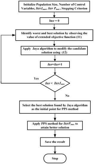
Figure 1.
Flowchart of proposed hybrid Jaya–PPS algorithm.
The computational steps of the hybrid Jaya–PPS algorithm are summarized as follows:
- Initialize the population with control variables and set maximum iteration count IterJmax and the number of iterations IterJmax for the PPS method.
- Set iteration Iter = 0.
- Identify the worst and best solutions in the population on the basis of the extended objective function value Equation (11).
- Modify the solutions using the best and the worst solutions Equation (12).
- If the modified solution is found to be better than the previous one, move to step vi, otherwise jump to step vii.
- Replace the previous solution with the modified one and jump to step viii.
- Retain previous solution.
- Increase iteration number by 1, i.e., Iter = Iter + 1.
- If Iter < IterJmax, then move to step iii, else move to step x.
- Select the best solution found by the Jaya algorithm as the initial point for the PPS method and apply the PPS method for IterPmax iterations to attain a better solution.
- Stop. Optimal solution achieved.
4. OPF Results and Discussion
In order to demonstrate the effectiveness of the proposed hybrid Jaya–PPS algorithm, DA, GWO, Jaya, J-PPS1, J-PPS2 and J-PPS3 algorithms were applied to the IEEE 30-bus system [6,23], IEEE 57-bus system [24] and IEEE 118-bus system for solving OPF problems with and without considering DG. The lower and upper limits of the 24 control variables, line data, bus data along with their initial settings for the IEEE 30-bus system, are taken from [23], while the emission and fuel cost coefficients are taken from [25]. In a combined single-objective function, the weight of an objective is proportional to the preference factor or weightage assigned to that objective function. This procedure is called a preference-based multi-objective optimization. For comparison, the combined objective function, COF, is obtained by considering the weighting factors WECM, WRPLM and WTVDM as 19, 22 and 21, respectively, as reported in [9]. The same procedure can be used for different systems also.
The IEEE 30-bus system is modified by including renewable energy source-based DG units. The optimal location for the DG unit is selected using the sensitivity of real power loss and the generation cost to each real and reactive power [6]; in this case, it was bus no. 30. At this bus, the capacity selected for the type 1 DG unit is 5 MW.
The IEEE 57-bus test system has 7 generators and 80 branches. The lower and upper voltage magnitude limits for all the generator and load buses of the system are considered to be 0.94 pu and 1.06 pu, respectively. The limits for the regulating transformers’ tap settings are taken as 0.9 pu and 1.1 pu. The generator coefficients, lower and upper limits of all the 33 control variables and system data (bus data, line data) along with their initial settings are taken from [24]. At 100 MVA base, the real power demand and reactive power demand of this test system are 12.508 pu and 3.364 pu, respectively. In the case of the IEEE 57-bus system, the combined objective function, COF, is obtained by considering the weighting factors WECM, WRPLM and WTVDM as 300, 30 and 600, respectively. IEEE 57-bus system is modified by inserting DG units [26]. The optimal locations of the type 1 DG units are bus nos. 35 and 36 with the capacities of 47.9067 MW and 47.2636 MW, respectively.
To evaluate the scalability of proposed algorithms and prove their efficacy to solve large-scale problems, all three variants of Jaya–PPS algorithms, the GWO and DA algorithm were applied to solve the OPF problem IEEE 118-bus system. The system data, generator coefficients, lower and upper limits of all the 130 control variables, along with their initial settings, are taken from [27]. The active and reactive power demands of this test system are 42.42 and 14.38 pu, respectively, at the 100 MVA base.
To demonstrate the effectiveness of the proposed algorithm, five cases considered are as follows:
- Case 1: OPF no DG in IEEE 30-bus test system.
- Case 2: OPF with DG in IEEE 30-bus test system.
- Case 3: OPF no DG in IEEE 57-bus test system.
- Case 4: OPF with DG in IEEE 57-bus test system.
- Case 5: OPF no DG in IEEE 118-bus system.
Various trials were carried out with different population sizes and no. of iterations. The best results thus achieved and reported in this paper are for population pop = 30 and no. of iterations Itermax = 200 for IEEE 30-bus test system and pop = 40 and Itermax = 300 for IEEE 57-bus test system. The OPF results with and without the inclusion of DG obtained using various EC and hybrid Jaya algorithms are included in this section. These algorithms were developed using MATLAB 13a version in a 3.6 GHz Intel Processor, 8 GB RAM Core i7 and 64-bit operating personal computer.
To compare the performance of various algorithms, all the algorithms were run for the same number of function evaluations (NFE), which is equal to 6000 in the case of the IEEE 30-bus test system and 12,000 in the case of the IEEE 57-bus test system. Details of the implementation of various algorithms and inclusion of PPS in the three variants of hybrid Jaya–PPS algorithms are given in Table 1.

Table 1.
Details of the DA, GWO, Jaya, J-PPS1, J-PPS2 and J-PPS3 algorithms.
4.1. Case 1: OPF No DG in IEEE 30-Bus Test System
In this case, the proposed hybrid Jaya–PPS algorithms, Dragonfly algorithm [28], GWO algorithm [29] and Jaya algorithm [21] were applied to solve the OPF problem considering the combined objective function without DG. Table 2 shows the results of these methods along with optimal control variable settings. The result clearly shows the superiority of the proposed J-PPS3 over other methods. Its combined objective function (965.0228) is less than those attained using other methods with no violation of the pre-specified constraints. The results of hybrid Jaya–PPS algorithms are compared with DA, GWO, Jaya algorithm and also with the reported results available in recent literature in Table 3.
Table 2.
OPF results with optimum values of control variables for IEEE 30-bus system.
Table 3.
Results of the proposed method and other methods for case 1.
From Table 3, it can be noted that the proposed J-PPS3 algorithm provides the minimum value of the combined objective function. This demonstrates the effectiveness of the proposed J-PPS3 algorithm as compared to DA, GWO, Jaya, J-PPS1 and J-PPS2 algorithms and other competitors [6,9,10,11]. Convergence characteristics of DA, GWO, Jaya, J-PPS1, J-PPS2 and J-PPS3 algorithms are shown in Figure 2, while Figure 3 displays the voltage profile provided by the proposed J-PPS3 algorithm. This figure shows that voltages magnitudes at all the buses are within the given upper and lower limits.
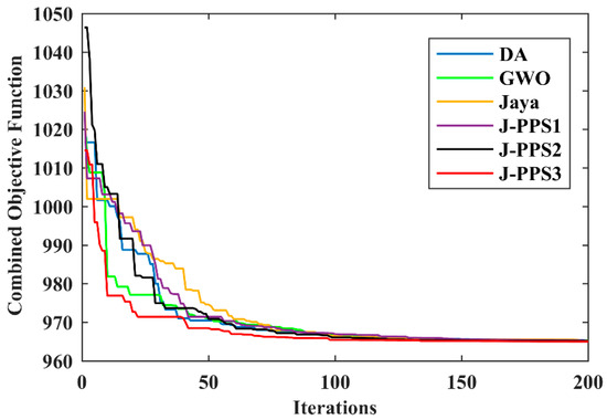
Figure 2.
Convergence characteristics for various algorithms for Case 1.
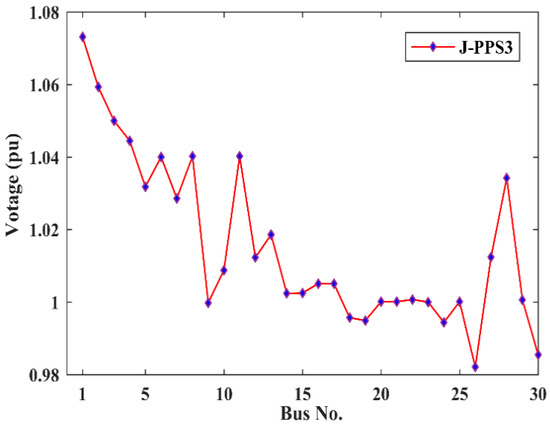
Figure 3.
Voltage profile provided by J-PPS3 for Case 1.
4.2. Case 2: OPF with DG in IEEE 30-Bus Test System
In this case, the DA, GWO, Jaya, J-PPS1, J-PPS2 and J-PPS3 algorithms were applied to solve the optimal power flow problem incorporating DG considering the minimization of fuel cost, real power loss, emission and total voltage deviation. Afterward, their results were compared to find the best algorithm. The results of this case for all the algorithms along with optimal control variable settings are shown in Table 4. The numerical outcomes in Table 4 demonstrate that the proposed J-PPS3 algorithm is more effective as compared to other approaches for solving the OPF problem with DG. The combined objective function value obtained using the J-PPS3 algorithm is 937.3486, which is less than those of the DA, GWO, Jaya, J-PPS1 and J-PPS2 methods without any violation of the limits.
Table 4.
OPF results with optimum values of control variables for the IEEE 30-bus system.
It should be noted that the combined objective function of the proposed J-PPS3 decreased from 965.0228 (Case 1) to 937.3486 by 2.86% after placing the DG as anticipated. Type 1 DG has been modeled as a negative load, and hence the total load demand is reduced. This further decreases the fuel cost and hence the combined objective function.
After integrating the DG, the convergence characteristics of DA, GWO, Jaya, J-PPS1, J-PPS2 and J-PPS3 algorithms are depicted in Figure 4. As can be observed from Figure 4, J-PPS3 provides fast and smooth convergence characteristics compared to the other methods. The voltage magnitudes at all the buses provided by the proposed J-PPS3 algorithm are shown in Figure 5, which are within the specified limits.
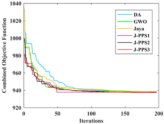
Figure 4.
Convergence characteristics for various algorithms for Case 2.
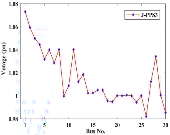
Figure 5.
Voltage profile provided by J-PPS3 for Case 2.
4.3. Case 3: OPF No DG in IEEE 57-Bus Test System
In this case, to evaluate the scalability of the J-PPS3 algorithm and to prove its efficacy to solve large scale problems, all six DA, GWO, Jaya, J-PPS1, J-PPS2 and J-PPS3 algorithms were applied to solve the OPF problem in the IEEE 57-bus test system with no DG placed in it. In this case, the combined objective function for OPF comprises fuel cost, emission, real power loss and total voltage deviation. The OPF results and the optimal control variable settings of the J-PPS3 algorithm are compared with DA, GWO, Jaya, J-PPS1 and J-PPS2 in Table 5. Table 6 displays the comparison of numerical outcomes of DA, GWO, Jaya, J-PPS1, J-PPS2 and J-PPS3 algorithms and the reported results [10,12] for the IEEE 57-bus system. Figure 6 displays the convergence characteristics of DA, GWO, Jaya, J-PPS1, J-PPS2 and J-PPS3 algorithms.
Table 5.
Optimum values of control variables for IEEE 57-bus system without DG.
Table 6.
OPF results of IEEE 57-bus system without DG.
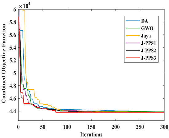
Figure 6.
Convergence characteristics for various algorithms for Case 3.
The results in Table 6 prove the dominance of the hybrid J-PPS3 algorithm over other EC-based and hybrid Jaya–PPS algorithms in solving the OPF problem for a large-size power system. The proposed J-PPS3 algorithm provided the combined objective function value as 43,788.631, which is better than the combined objective functions offered by other algorithms with no constraint violation. The bus voltages profile obtained using the J-PPS3 algorithm is within specified limits, as shown in Figure 7.
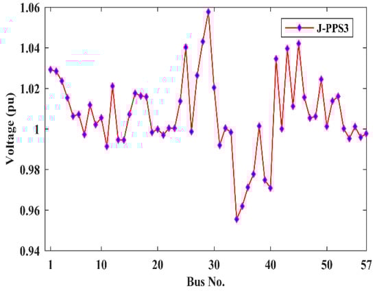
Figure 7.
Voltage profile provided by J-PPS3 for Case 3.
4.4. Case 4: OPF with DG in IEEE 57-Bus Test System
In this case, to establish the effectiveness of the J-PPS3 algorithm for solving the OPF problem, the IEEE 57-bus test system with two DGs [26] is considered. The obtained results and the optimal control variable settings of the J-PPS3 algorithm are compared with those of DA, GWO, Jaya, J-PPS1 and J-PPS2 algorithms in Table 7.
Table 7.
OPF results for IEEE 57-bus system with two DGs.
The results in Table 7 prove the dominance of the proposed hybrid J-PPS3 algorithm over other EC-based and hybrid Jaya–PPS algorithms in successfully handling the OPF problem in large-scale systems penetrated with two DG units. The proposed J-PPS3 algorithm provided the combined objective function value as 39,136.324, which is better than the combined objective functions offered by other algorithms without violating the constraints. The combined objective function of J-PPS3 decreased from 43,778.631 (Case 3) to 39,136.324 (by 10.60%) after implanting two DGs as expected.
In this case, the proposed J-PPS3 algorithm also provided fast and smooth convergence characteristics compared to other algorithms, as shown in Figure 8. The bus voltages profile obtained by the J-PPS3 algorithm is within limits, as shown in Figure 9.
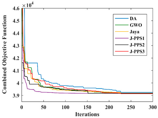
Figure 8.
Convergence characteristics for various algorithms for Case 4.
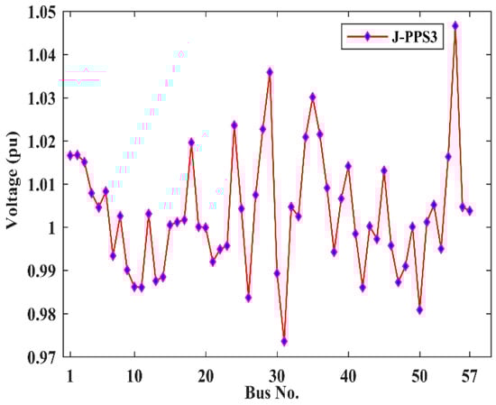
Figure 9.
Voltage profile provided by J-PPS3 for Case 4.
4.5. Case 5: OPF No DG in IEEE 118-Bus System
In Case 5, fuel cost is selected as the main objective. The minimum fuel cost obtained by the J-PPS3 algorithm is 129,507.6123 $/h, while the minimum fuel cost obtained by J-PPS2 and J-PPS1 algorithms is 129,821.4309 $/h and 129,961.8924 $/h, respectively. The minimum fuel cost obtained using hybrid Jaya–PPS algorithms and other meta-heuristic algorithms are depicted in Table 8. From Table 8, it is clear that the fuel cost obtained from J-PPS3 algorithm is the least compared to other methods, demonstrating the effectiveness of the proposed J-PPS3 algorithm compared to the J-PPS2, J-PPS1, DA, GWO algorithms and other competitors in handling the OPF problem in a large-sized power system. The fuel cost characteristics for Case 5 are shown in Figure 10.
Table 8.
Case 5 (Fuel cost minimization) results in IEEE 118-bus system.
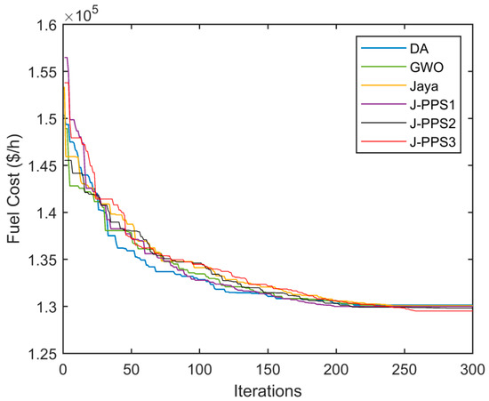
Figure 10.
Convergence characteristics for various algorithms for Case 5.
5. Statistical Analysis
Statistical analysis was carried out to evaluate the robustness of DA, GWO, Jaya, J-PPS1, J-PPS2 and J-PPS3 algorithms to solve the OPF problem with and without DG. A total of 50 independent trials were carried out with the same population size and same no. of function evaluations for each case. As previously mentioned, the population sizes and the maximum NFE were 30 and 6000 for the IEEE 30-bus test system, respectively, and as 40 and 12,000 for the IEEE 57-bus system, respectively, which provided the best results. These trials were utilized to find out the best value, worst value, average (mean) value of OPF results and standard deviation (SD) required for statistical analysis of various algorithms implemented in this paper and are shown in Table 9 and Table 10, respectively. These tables show that, for all the considered cases of IEEE 30-bus and IEEE 57-bus test systems, the best, worst and mean values are nearest to each other; therefore, the standard deviation values are low. The smallest SD values offered by the proposed J-PPS3 algorithm in all the cases clearly indicate that statistically meaningful results are obtained by the proposed J-PPS3 method. This affirms the robustness of the proposed algorithm.
Table 9.
Performance measures of various algorithms for IEEE 30-bus system.
Table 10.
Performance measures of various algorithms for IEEE 57-bus system.
6. Conclusions
This paper proposes a hybrid Jaya–PPS algorithm using Jaya and Powel’s Pattern Search method to solve the multi-objective optimal power flow problem incorporating DG to minimize generation fuel cost, emission, real power loss and voltage profile improvement simultaneously. The multi-objective optimization problem has been solved by transforming it into a single-objective optimization problem using weighting factors. Three versions of hybrid Jaya–PPS techniques J-PPS1, J-PPS2 and J-PPS3, were developed by integrating the PPS method in different ways. In order to evaluate the performance of the proposed hybrid Jaya–PPS algorithms, these algorithms were employed to solve the OPF problem in standard IEEE 30-bus and IEEE 57-bus systems with/without DG and IEEE 118-bus systems for fuel cost minimization. The results achieved by the hybrid Jaya–PPS algorithms were compared to the Dragonfly algorithm, Grey Wolf Optimization and Jaya algorithms, and the reported results published in recent literature. The numerical outcomes demonstrate that the proposed J-PPS3 algorithm dominates other approaches when solving the OPF problem. For example, the combined objective function found by Jaya–PPS1 for the 30-bus system is 937.3486, with a reduction of 2.86% of the original system, with a 0.01105 standard deviation. This benefit increases further with the size of the system. Statistical analysis has shown that the hybrid J-PPS3 algorithm is a reliable and robust optimization algorithm. As the hybrid J-PPS3 algorithm has good exploration and exploitation properties, it can reliably solve the OPF problem in practical power systems.
Author Contributions
All authors have contributed equally in technical and non-technical work. All authors have read and agreed to the published version of the manuscript.
Funding
This research received no external funding.
Institutional Review Board Statement
Not applicable.
Informed Consent Statement
Not applicable.
Data Availability Statement
Not applicable.
Conflicts of Interest
The authors declare no conflict of interest.
Nomenclature
| W | dependent variable |
| X | control variable |
| M (W, X) | objective function |
| g (W, X) & h (W, X) | equality and inequality constraints |
| NB | number of buses |
| NLB | number of load buses |
| Ntl | number of transmission lines |
| NGN | numbers of generators |
| NC | number of VAR compensation units |
| NTR | number of regulating transformers |
| and | active and reactive load |
| and | Active & reactive power generations |
| and | real and reactive power loss |
| and | minimum & maximum voltage limits of kth generator bus |
| minimum and maximum limits of reactive power output of kth generator | |
| minimum and maximum active power limits of kth generating unit | |
| and | maximum and minimum tap setting of kth transformer |
| maximum and minimum voltage limit of kth load bus | |
| maximum MVA flow in kth transmission line | |
| , , and | penalty factors corresponding to limit violations |
| , and | fuel cost coefficients of the ith generating unit |
| slack bus generator’s active power output | |
| emission coefficients of ith generating unit | |
| pop | Population size |
| Itermax | Maximum No. of iterations |
| IterJmax | Maximum No. of Jaya iterations |
| IterPmax | Maximum No. of PPS iterations |
| NFE | Number of function evaluations |
| JFE | Number of Jaya Function Evaluations |
| PSFE | Number of PPS Function Evaluation |
References
- Carpentier, J. Optimal power flows. Int. J. Electr. Power Energy Syst. 1979, 1, 3–15. [Google Scholar] [CrossRef]
- Hazra, J.; Sinha, A.K. A multi-objective optimal power flow using particle swarm optimization. Eur. Trans. Electr. Power 2010, 21, 1028–1045. [Google Scholar] [CrossRef]
- Bouchekara, H.; Abido, M.; Chaib, A.; Mehasni, R. Optimal power flow using the league championship algorithm: A case study of the Algerian power system. Energy Convers. Manag. 2014, 87, 58–70. [Google Scholar] [CrossRef]
- Quadri, I.A.; Bhowmick, S.; Joshi, D. A comprehensive technique for optimal allocation of distributed energy resources in radial distribution systems. Appl. Energy 2018, 211, 1245–1260. [Google Scholar] [CrossRef]
- Khaled, U.; Eltamaly, A.M.; Beroual, A. Optimal Power Flow Using Particle Swarm Optimization of Renewable Hybrid Distributed Generation. Energies 2017, 10, 1013. [Google Scholar] [CrossRef]
- Elattar, E.E.; ElSayed, S.K. Modified JAYA algorithm for optimal power flow incorporating renewable energy sources considering the cost, emission, power loss and voltage profile improvement. Energy 2019, 178, 598–609. [Google Scholar] [CrossRef]
- Srivastava, L.; Singh, H. Hybrid multi-swarm particle swarm optimisation based multi-objective reactive power dispatch. IET Gener. Transm. Distrib. 2015, 9, 727–739. [Google Scholar] [CrossRef]
- Low, S.H. Convex Relaxation of Optimal Power Flow—Part I: Formulations and Equivalence. IEEE Trans. Control. Netw. Syst. 2014, 1, 15–27. [Google Scholar] [CrossRef]
- Khelifi, A.; Bentouati, B.; Chettih, S. Optimal Power Flow Problem Solution Based on Hybrid Firefly Krill Herd Method. Int. J. Eng. Res. Afr. 2019, 44, 213–228. [Google Scholar] [CrossRef]
- Ghasemi, M.; Ghavidel, S.; Ghanbarian, M.M.; Gharibzadeh, M.; Vahed, A.A. Multi-objective optimal power flow considering the cost, emission, voltage deviation and power losses using multi-objective modified imperialist competitive algorithm. Energy 2014, 78, 276–289. [Google Scholar] [CrossRef]
- Mohamed, A.-A.A.; Mohamed, Y.S.; El-Gaafary, A.A.; Hemeida, A.M. Optimal power flow using moth swarm algorithm. Electr. Power Syst. Res. 2017, 142, 190–206. [Google Scholar] [CrossRef]
- Biswas, P.P.; Suganthan, P.N.; Mallipeddi, R.; Amaratunga, G.A.J. Multi-objective optimal power flow solutions using a constraint handling technique of evolutionary algorithms. Soft Comput. 2019, 24, 2999–3023. [Google Scholar] [CrossRef]
- Alsumait, J.; Sykulski, J.; Al-Othman, A. A hybrid GA–PS–SQP method to solve power system valve-point economic dispatch problems. Appl. Energy 2010, 87, 1773–1781. [Google Scholar] [CrossRef]
- Attaviriyanupap, P.; Kita, H.; Tanaka, E.; Hasegawa, J. A hybrid EP and SQP for dynamic economic dispatch with nonsmooth fuel cost function. IEEE Trans. Power Syst. 2002, 17, 411–416. [Google Scholar] [CrossRef]
- Narang, N.; Dhillon, J.S.; Kothari, D.P. Multi-objective fixed head hydrothermal scheduling using integrated predator-prey optimization and Powell search method. Energy 2012, 47, 237–252. [Google Scholar] [CrossRef]
- Mahdad, B.; Srairi, K. Multi objective large power system planning under sever loading condition using learning DE-APSO-PS strategy. Energy Convers. Manag. 2014, 87, 338–350. [Google Scholar] [CrossRef]
- Ben Hmida, J.; Chambers, T.; Lee, J. Solving constrained optimal power flow with renewables using hybrid modified imperialist competitive algorithm and sequential quadratic programming. Electr. Power Syst. Res. 2019, 177, 105989. [Google Scholar] [CrossRef]
- Wu, J.; Wei, Z.; Li, W.; Wang, Y.; Li, Y.; Sauer, D.U. Battery Thermal- and Health-Constrained Energy Management for Hybrid Electric Bus Based on Soft Actor-Critic DRL Algorithm. IEEE Trans. Ind. Inform. 2021, 17, 3751–3761. [Google Scholar] [CrossRef]
- Wu, J.; Wei, Z.; Liu, K.; Quan, Z.; Li, Y. Battery-Involved Energy Management for Hybrid Electric Bus Based on Expert-Assistance Deep Deterministic Policy Gradient Algorithm. IEEE Trans. Veh. Technol. 2020, 69, 12786–12796. [Google Scholar] [CrossRef]
- Taher, M.A.; Kamel, S.; Jurado, F.; Ebeed, M. An improved moth-flame optimization algorithm for solving optimal power flow problem. Int. Trans. Electr. Energy Syst. 2019, 29, e2743. [Google Scholar] [CrossRef]
- Rao, R.V. Jaya: A simple and new optimization algorithm for solving constrained and unconstrained optimization problems. Int. J. Ind. Eng. Comput. 2016, 7, 19–34. [Google Scholar] [CrossRef]
- Rao, S.S. Engineering Optimization: Theory and Practice; John Wiley & Sons: Hoboken, NJ, USA, 2019. [Google Scholar]
- Lee, K.Y.; Park, Y.M.; Ortiz, J.L. A united approach to optimal real and reactive power dispatch. IEEE Trans. Power Appar. Syst. 1985, PAS-104, 1147–1153. [Google Scholar] [CrossRef]
- Zimmerman, R.D.; Murillo-Sánchez, C.E.; Thomas, R.J. Matpower. Available online: https://matpower.org/docs/ref/matpower5.0/case57.html (accessed on 11 May 2021).
- Niknam, T.; Narimani, M.R.; Jabbari, M.; Malekpour, A.R. A modified shuffle frog leaping algorithm for multi-objective optimal power flow. Energy 2011, 36, 6420–6432. [Google Scholar] [CrossRef]
- Charles, J.K.; Odero, N.A. Effects of distributed generation penetration on system power losses and voltage profiles. Int. J. Sci. Res. Publ. 2013, 3, 1–8. [Google Scholar]
- Power System Test Cases. Available online: http://www.ee.washington.edu/research/pstca (accessed on 11 May 2021).
- Meraihi, Y.; Ramdane-Cherif, A.; Acheli, D.; Mahseur, M. Dragonfly algorithm: A comprehensive review and applications. Neural Comput. Appl. 2020, 32, 16625–16646. [Google Scholar] [CrossRef]
- Mirjalili, S.; Mirjalili, S.M.; Lewis, A. Grey Wolf Optimizer. Adv. Eng. Softw. 2014, 69, 46–61. [Google Scholar] [CrossRef]
- Jiang, Q.; Geng, G.; Guo, C.; Cao, Y. An Efficient Implementation of Automatic Differentiation in Interior Point Optimal Power Flow. IEEE Trans. Power Syst. 2009, 25, 147–155. [Google Scholar] [CrossRef]
- Brust, J.J.; Anitescu, M. Convergence Analysis of Fixed Point Chance Constrained Optimal Power Flow Problems. arXiv 2021, arXiv:2101.11740. [Google Scholar]
- Fortenbacher, P.; Demiray, T. Linear/quadratic programming-based optimal power flow using linear power flow and absolute loss approximations. Int. J. Electr. Power Energy Syst. 2019, 107, 680–689. [Google Scholar] [CrossRef]
- Singh, R.P.; Mukherjee, V.; Ghoshal, S. Particle swarm optimization with an aging leader and challengers algorithm for the solution of optimal power flow problem. Appl. Soft Comput. 2016, 40, 161–177. [Google Scholar] [CrossRef]
- Radosavljević, J.; Klimenta, D.; Jevtić, M.; Arsić, N. Optimal Power Flow Using a Hybrid Optimization Algorithm of Particle Swarm Optimization and Gravitational Search Algorithm. Electr. Power Compon. Syst. 2015, 43, 1958–1970. [Google Scholar] [CrossRef]
- Roberge, V.; Tarbouchi, M.; Okou, F. Optimal power flow based on parallel metaheuristics for graphics processing units. Electr. Power Syst. Res. 2016, 140, 344–353. [Google Scholar] [CrossRef]
Publisher’s Note: MDPI stays neutral with regard to jurisdictional claims in published maps and institutional affiliations. |
© 2021 by the authors. Licensee MDPI, Basel, Switzerland. This article is an open access article distributed under the terms and conditions of the Creative Commons Attribution (CC BY) license (https://creativecommons.org/licenses/by/4.0/).