Impact of Renewable Energy Sources on Power System Flexibility Requirements

Abstract

A power system can be defined as flexible if it can within economic and technological boundaries respond quickly and adequately to variations in supply and demand. The ongoing penetration of variable and intermittent renewable energy sources (RES) like wind and solar imposes additional and more critical requirement on power system flexibility. In this paper we propose a method to quantify these requirements based on the comparison of seven demand side parameters describing the statistical properties of the net load and the residual load of the referred power system. Each one of these parameters reflects a separate requirement on the available conventional generation in hourly and daily time scales—ramp up and ramp-down capabilities, technological minimum of generation, daily variation of generation. The proposed approach can be used to predict the requirements for generation flexibility according to the expected scenario of RES penetration in the future development of energy power system. It has been applied and integrated from the Bulgarian Transmission System Operator (TSO) which name is the Bulgarian Electricity System Operator (ESO).

1. Introduction

The term flexibility has been only recently introduced in power systems and immediately garnered tremendous interest [1]. The need for operational flexibility is also increasing [2]. Despite its importance, flexibility has not been globally defined and it has been approached differently in several studies in the literature.

In the literature, flexibility has been distinguished in two main categories namely, planning and operational flexibility with the latter being in the scope of most studies. Planning flexibility mainly concerns long term planning associated with transmission system design [3]. On the other hand, operational flexibility is related to the equipment of generation system and to its real time response in power changes through optimized controllability [4]. Furthermore, since the interconnections of power systems that serve different countries or areas and operated by different Transmission System Operators (TSOs) have been dramatically increased, the term “exported flexibility” emerged. This term defines the operating flexibility that a TSO can offer to a neighbor network through the tie-points [5]. The general definition of flexibility in [6] is assumed to be more accurate and defines flexibility as “the ability of a system to deploy its resources to respond to changes in net load”. Concluding, flexible power systems must have adequate resources, optimized operation and planning management [1].

Recently in the context of the BRIDGE initiative, flexibility has been given special attention especially in relation with the distribution grid turning into a supply driven system, placing decentralized producers and consumers in the center of the transmission system. The flexibility concept in this, let’s say, ‘bottom up’, in the voltage level sense, approach has been defined as:

• Solutions to continually guarantee the balance of power generation and consumption within the distribution grid in order to preserve its stability therefore increasingly rest on the deployment and exploitation of operational flexibility [6];
• On the one hand, operational flexibility comprises the usage of energy storage systems, such as battery, gas, water or multi-energy carrier storage [7];
• On the other hand, operational flexibility resources are also accessed by flexible controllable consumption and generation units in terms of Demand Side Management and Demand Response mechanisms, for instance on a residential city district level [8,9].

In this context, the Expert Group 3 of the Smart Grid Task Force of the European Commission [9] defines the term flexibility in the following way: “On an individual level, flexibility is the modification of generation injection and/or consumption patterns in reaction to an external (signal or activation) in order to provide services within the energy system”.

Since flexibility has been identified as an essential property of power systems, indices and metrics that can be used to identify and evaluate a power system flexibility are continually defined. Some already developed indices and metrics are Inflexibility Signs [10]; Flexibility Chart [11]; GIVAR, Flexibility assessment tool (FAST2) [12]; Insufficient ramping resource expectation (IRRE) [13]; Normalized flexibility index (NFI) [14]; Loss of wind estimation (LOWE) [15]; Lack of ramp probability (LORP) [16], Locational flexibility [17], Ranking approach [18].

The uncertain nature of large-scale integration of variable renewable energy makes it technically challenging [19,20,21]. In general, the generation portfolio is designed in such a way that provides enough flexibility to cope with the variability of RES in the most efficient manner managing load forecast error and unplanned generation outages. Due to variable renewable sources like for instance wind and photovoltaic power the generation capacity increases. Therefore, the system needs to be able to address the variability and unpredictability associated with these sources [22]. The necessity to provide additional flexibility while integrating large penetrations of intermittent generation got its recognition from a central point of view. This issue, however, requires the view of the participants in electricity markets [23]. Such participants could be flexibility providers or potential providers. They will be able to provide this flexibility when this returns an economic profit [24].

In this paper we argue the following: One system is more flexible than another one if it is able to accommodate more RES without limits, under the condition that there is the same demand and available RES generation. The variations of wind and PV are measured as follows: seconds, minutes, hours, days, months, seasons and years. The aim is to manage the daily net load cycle.

The focus of this work is on flexibility on an hourly and daily basis. The paper does not analyze weekly and seasonal flexibility. It will be a subject of a further work. Variability and uncertainty are the two characteristics of wind and PV generation that drive the need for flexibility.

Frequent and natural fluctuations in wind and PV output pose challenges to conventional generators. This is dictated by the need for fast sudden and large ramping and frequent start-ups. The need for reserves is triggered by the unavoidable errors between wind and PV generation forecasts and actual outputs. Hence to properly accommodate large volumes of wind and PV power, the system has to be highly flexible to follow the variable net demand and cope with the uncertainties.

These requirements are usually fulfilled by flexible generation, energy storage, and flexible demand (demand side management). On the basis of these three basic options for providing the flexibility needed, different metrics for quantification are applied.

In the joint report of the OECD and IEA [25], the ability of the power system to modify generation and consumption in response to expected and unexpected variability is referred to as flexibility [26]. It further classifies the flexibility needs into 3 basic groups: flexibility for power, energy and transfer capacity [26]. There are different definitions for power system flexibility which reflect and emphasize on different requirement on the conventional generation from operational perspective [27,28,29,30,31]. Generation system flexibility is quantified by three main indicators—absolute power output range (MW), ramp rate (MW/min), and power output continuity (energy) (MWh) [32].

2. Power System Probabilistic Approach for Flexibility Assessment

Maintaining the admissible voltage levels is of utmost importance for all participants in the Electricity Energy System (EES) to reach good economic parameters. Since the development of EES is made in line with a ten-year plan which is also in conformity with the plans of the neighboring countries for ensuring safe and reliable work of the Bulgarian EES in parallel with the European one, it would be beneficial to develop common rules to stimulate users and consumers to participate more actively in the regulation of EES, both in normal as well as emergency modes. This will increase the flexibility, the cross-border power exchange and it will improve transparency and provide for better planning of loads and generating capacities.

The challenges in front of the Bulgarian energy system are:

• Most of the Variable Renewable Energy (VRE) spread in BG is far from the load and in areas with remote access. Photovoltaics are main part of VRE but the forecast of their generation is still not sufficient;
• The main flexible resources are provided form coal and hydro power stations;
• Coal fired plants comprise a significant portion of the generation mix in Bulgaria. During peak hours, most of them operate at maximum output or mid-merit, and the system has fairly good ability to meet upward net load variations in short term. During times of minimum demand though, a significant portion of coal power plants are offline and their technical characteristics (namely start-up time) do not allow them to offer flexibility in the 6 h time horizon.

There are also three main indicators which reflect and measure the problems with RES. The variations of these indicators of which together with the increase of the total installed capacity from wind power plants (WPP) and photovoltaic power plants (PvPP) will predetermine the rising requirements for the regulating capacities and the commitment of the generating units:

• The increase in the standard deviation of the hourly fluctuations of the residual load along with the increase of the total installed capacity from wind and PV also determines the necessary increase of the respective operational reserve (aFRR—automatic Frequency Restoration Reserves, mFRR—manual frequency restoration reserves and RR—Replacement Reserves used to restore/support the required level of FRR) to cover these fluctuations with a set probability corresponding to the adopted level of security of supply;
• The increase in the diurnal range of negative and positive variation of the residual load with an increase in the total installed capacity from wind and PV determines, in turn, the required extension of the diurnal total regulating range supplied from conventional generators;
• The increase in the total installed capacity from wind and PV leads to proportional reduction of the minimum residual load to be “covered” by the conventional generating capacities.

Depending on the type, structure, ratio and operational parameters of the available conventional generators in the EPS, one of the above three indicators will determine maximum amount of total installed capacity from WPPs and PvPPs that can be seamlessly integrated into the EPS, i.e., determining the most restrictive indicator from the above mentioned: available operational reserve (aFRR, mFRR and RR) within an hour; available diurnal regulating range or the ability to “cover” the minimum loads.

A number of statistical approaches and methods are used to quantify the influence and “contribution” of WPPs and PvPPs on the enhancement of random factors in the operation of the EPS. This assessment is based on the quantitative comparison of all defining factors of the energy regime / operating state obtained for the total and residual load or for two variants of the residual load received for different values of the installed wind and PV capacities.

The variation in the power output from WPPs and PvPPs over time is a purely random process with continuously changing probability characteristics and indicators depending on the change in the “availability” of the respective renewable energy resources—wind and sun. The two random processes defining the mode of operation of the conventional generators are respectively:

• The time series of the hourly loads of the EPS denote with Pi;
• The corresponding time series of the total power output from wind and PV denote with RESi.

The residual or so-called net load is the part of the total system load that has to be “covered” by conventional generating capacities in the power system and is calculated as difference:

$$P_i^{res}=P_i-RE{S}_i,$$

(1)

i.e., in this case, the cumulative wind and PV power output is seen as a “negative” load. The resulting statistical time series $P_i^{res}$ is also a random process whose equivalent probability characteristics [30] and metrics are derived from those of the two random processes that form it, the Theorems and Laws should be stated. It has already been pointed out that the hourly fluctuations of the load and the power output of WPPs and PvPPs have a normal probability distribution. Under this condition the standard deviation of the residual load will be determined by the formula:

$${\sigma }_{p-res}^2={\sigma }_p^2+{\sigma }_{res}^2\mp 2R\frac{p}{res}{\sigma }_p^{}{\sigma }_{res}^{},$$

(2)

where ${\sigma }_{p-res}^{}$—Standard deviation of the residual load; ${\sigma }_p^{}$ σ—Standard deviation of the total load; ${\sigma }_{res}^{}$—Standard deviation of the cumulative output from WPPs and PvPPs and $R\frac{p}{res}$—Correlation coefficient between the two processes.

Based on the value of the correlation coefficient the following options are possible:

When:

$$R\frac{p}{res}=0 \to {\sigma }_{p-res}^2={\sigma }_p^2+{\sigma }_{res}^2$$

When:

$$R\frac{p}{res}>0 \to {\sigma }_{p-res}^2>\left({\sigma }_p^2+{\sigma }_{res}^2\right)$$

When:

$$R\frac{p}{res}<0 \to {\sigma }_{p-res}^2<\left({\sigma }_p^2+{\sigma }_{res}^2\right)$$

When:

$$R\frac{p}{res}=1 \to {\sigma }_{p-res}^2=\left({\sigma }_p^2+{\sigma }_{res}^2+2R{\sigma }_p^{}{\sigma }_{res}^{}\right)$$

When:

$$R\frac{p}{res}=-1 \to {\sigma }_{p-res}^2=\left({\sigma }_p^2+{\sigma }_{res}^2-2R{\sigma }_p^{}{\sigma }_{res}^{}\right)$$

The values of the correlation coefficients between the two processes and the verification of their significance indicate that these processes can be considered independent, therefore the first ratio is in effect. However, in cases of significant correlation, the calculation will be performed according to the corresponding formula shown. As a result, the standard deviation of the residual load will always be greater than the standard deviation of the total (primary) load of the EPS. The difference:

$$\Delta {\sigma }_{res-impact\_IMPACT}={\sigma }_{p-res}-{\sigma }_p,$$

(3)

represents the total “contribution” of wind and PV to the increase in the standard deviation of the residual load and the consequent need to increase the requirements for the regulating reserves. This approach is used in the algorithm proposed below for assessing the joint impact of WPPs and PvPPs.

The quantification of this impact on the energy regimes/operating states is based on a comparison of the statistical and probability characteristics of the total load and the residual load resulting from the subtraction of the WPPs and PvPPs output. This comparison is carried out through scenario-based simulations with a gradual increase of the installed capacity from wind and PV, which models the expected development of the total installed capacity on the one hand and on the other the tendency and sensitivity of the energy regime’s/operating state’s parameters to this development. As already mentioned, the energy regime/operating state of the EPS is identified by the dynamic change in the power output of the synchronous units in operation and the change in their number according to the constantly altering operating conditions of the EPS:

• The random process of load variation;
• The random process of generation capacity availability due to forced outages of generating equipment;
• The random process of variation of wind and solar power as well as production from run-of-the-river HPPs.

Due to the influence of a number of persistent and occasional factors, the electrical consumption in each power system is constantly changing in all time slots—from several years to several seconds—which is a typical non-stationary random process. Reliable maintenance of the balance between production and consumption is the main goal of planning and control of the power system’s energy regimes. To achieve this, it is necessary to continuously adjust the operating power of the system in accordance with the change in the total load and the unexpected failures of the generating equipment. Depending on the speed and direction of this change different types of reserve “located” on generators with different maneuvering features and operating states must be activated or deactivated. The selective start-up of a particular unit and the regulation of its operating power is only possible with conventional generating units—thermal and hydro (reservoir and daily compensators) where the primary energy carrier is virtually always available as its availability can be stored and controlled. Unlike the wind, photovoltaic and run-of-the-river hydro power stations, where the change in power output happens only with a change in the intensity of the corresponding primary energy resource. These generating sources cannot be run selectively but only when there is sufficient primary resource, i.e., they are virtually non-dispatchable, and the electricity generated by them must be “absorbed” by the system at the time of its “emergence” and regardless of the frequency and amplitude with which it occurs (so-called “must take-energy”). For these reasons, the task of maintaining the balance in an EPS becomes more difficult, because besides the random fluctuations of the load and its predicted error, the power fluctuations of the renewable energy sources—wind, photovoltaic and run-of-the-river hydro must be compensated as well.

3. Case Study

The comparative analysis of the basic statistical indicators and characteristics of the total and residual load of the EPS is performed under the following conditions:

(1)

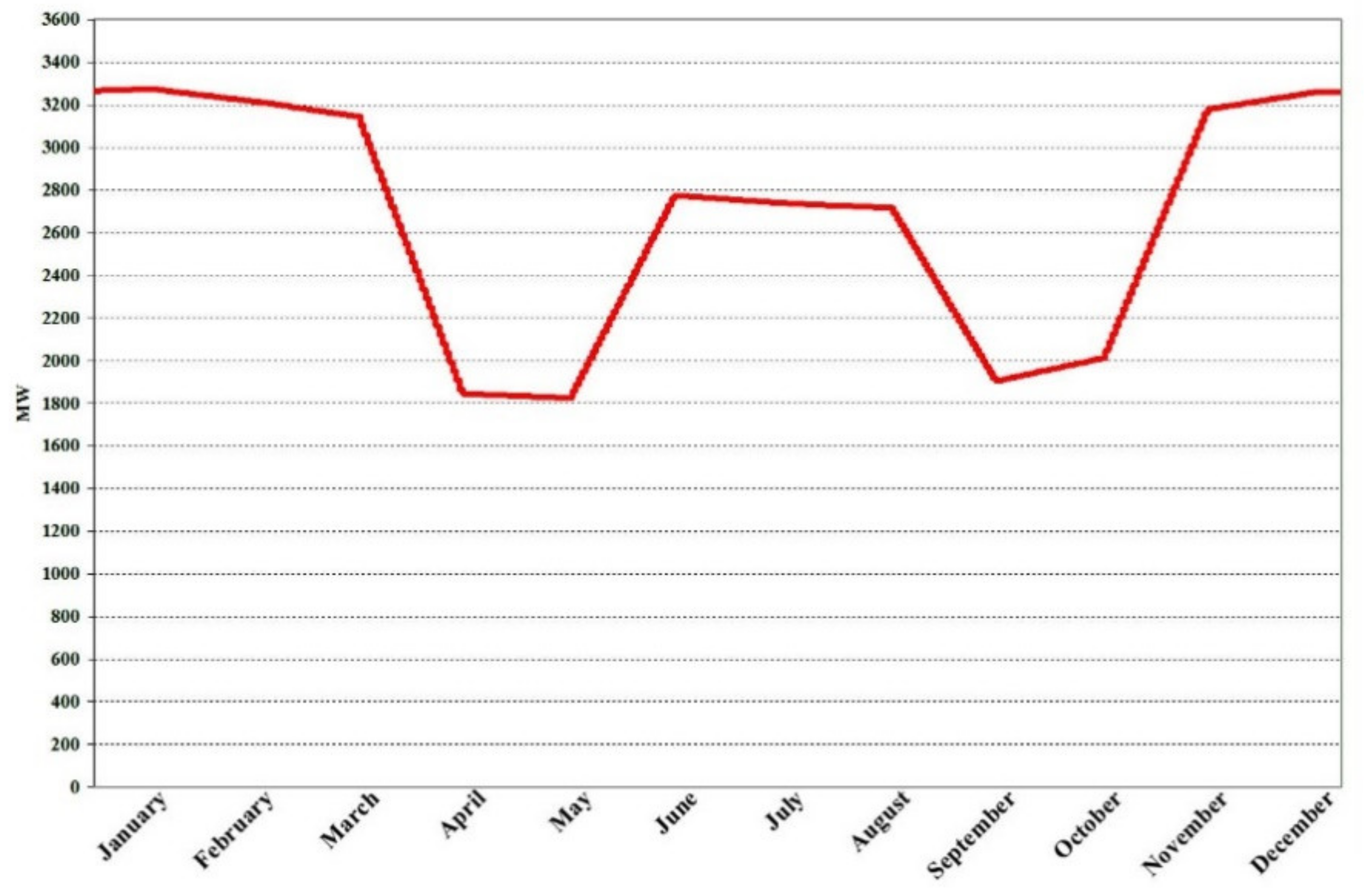
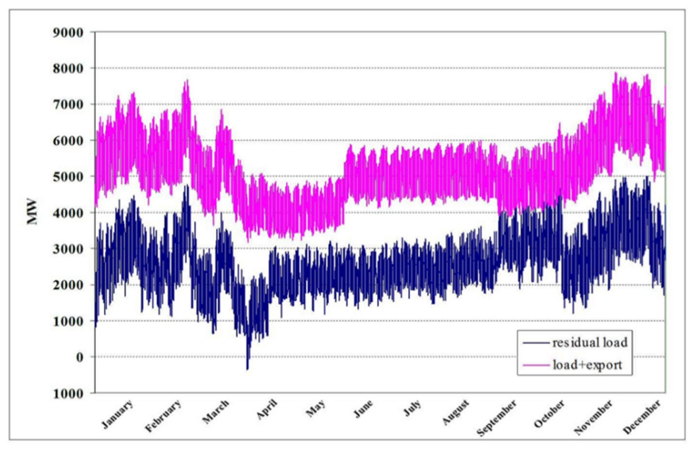
Gross total load—realized hourly loads (power plants’ auxiliary consumption included) of Bulgaria for 2014 with total annual electricity consumption of 36,875,896 MWh, without taking into account the potential export of electricity.

(2)

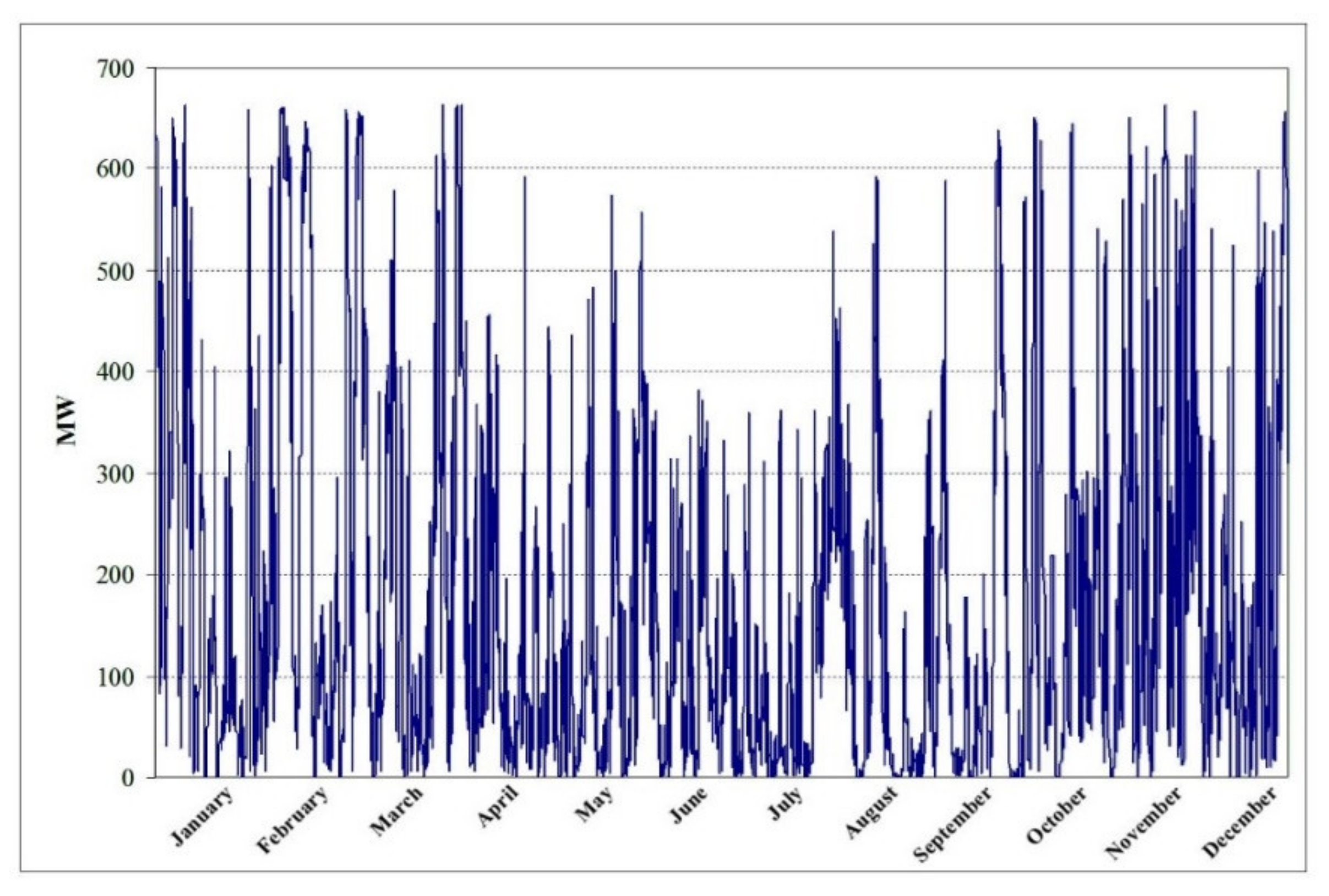
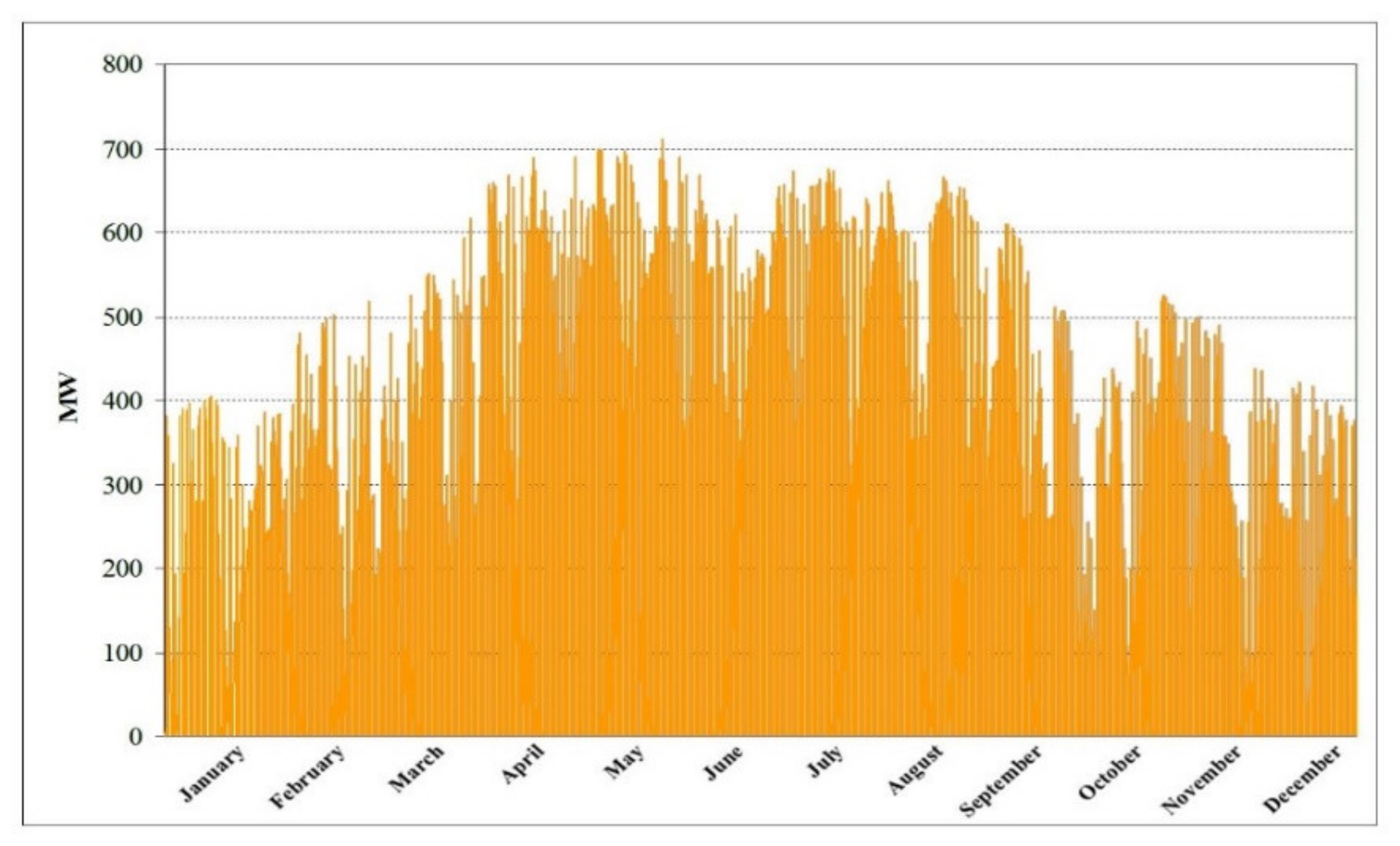
Realized hourly generations from WPPs and PvPPs in Bulgaria for 2019 (with installed capacities valid by 31 December 2019: WPPs = 701 MW and PvPPs = 1039 MWp).

(3)

The resulting residual load, as already indicated, is defined as the difference between the total gross hourly load and the corresponding total hourly generation from WPPs and PvPPs.

Table 1. Indicators between both types of loads ¹.

Day with:	Gross Total Load	Residual Load	Difference %
highest consumption, MWh	145,523	139,491	−6032.4	−4.1
lowest consumption, MWh	78,339	68,167	−10,171	−13.0
highest maximum load, MW	7106	6699	−407.03	−5.7
lowest maximum load, MW	3747	3558	−188.17	−5.0
lowest minimum load, MW	2656	2285	−371.66	−14.0
highest minimum load, MW	4890	4695	−195.07	−4.0
highest difference between maximum and minimum load, MW	2672	2686	14.2454	0.5
lowest difference between maximum and minimum load, MW	920	947	26.6213	2.9
highest density coefficient of the load profile	0.9161	0.8811	−0.035	−3.8
lowest density coefficient of the load profile	0.7566	0.6943	−0.0623	−8.2
highest hourly ramp up rate of the load, MW/h	724	753	28.9324	4.0
highest hourly ramp down rate of the load, MW/h	−686	−734	−48.721	7.1
largest standard deviation of the hourly fluctuations, MW	311	326	14.7274	4.7
smallest standard deviation of the hourly fluctuations, MW	141	141	−0.3035	−0.2
longest series of consecutive increase of the hourly load	11	15	4	36.3
longest series of consecutive decrease of the hourly load	11	11	0	0
largest value within a series of hourly load increase, MW	2017 (8)	2123 (7)	106	5.2
largest value within a series of hourly load decrease, MW	−2283 (9)	−2416 (9)	133	5.8

¹ The data is provided from the Electricity System Operator.

shows the extreme indicators between both types of loads as well as the respective nominal and percentage differences.

In

Table 2. Average annual values of the main indicators ².

Yearly Average Value of:	Gross Total Load	Residual Load	Difference
			%
daily demand, MWh	101,030	94,065	−6964.9	−6.9
daily maximum load, MW	4986	4841	−145.1	−2.9
daily minimum load, MW	3320	3144	−176.94	−5.3
difference between maximum and minimum load in a single day, MW	1665	1697	31.839	1.9
density coefficient of the load profile (Pave/Pmax)	0.846	0.809	−0.0369	−4.4
highest hourly ramp up rate of the load in a single day, MW/h	431	424	−6.8265	−1.6
highest hourly ramp down rate of the load in a single day, MW/h	−408	−416	−8.262	2.0
standard deviation of the hourly fluctuations of the load, MW	214	223	9.2246	4.3

² The data is provided from the Electricity System Operator.

for comparison purposes are also shown the average annual values of the main indicators and their nominal and percentage differences.

As additional, but very useful and expressive indicators, the following dimensions are introduced:

• $N_{abs.min}$—number of hours in the year in which the residual load is lower than the absolute minimum annual gross total load;
• $N_{min.gen}$—number of hours in the year in which the residual load is lower than the corresponding minimum admissible generation.

The minimum generation or the minimum admissible total operating power is determined in accordance to the mode of operation of each generation technology type. The minimum admissible generation values for the Bulgarian power system are shown on Figure 1 in hourly resolution.

The resulting $N_{abs.min}$ and $N_{min.gen}$ values for the residual load considered here are shown in

Table 3. Residual load—initial conditions.

Residual Load	Hours
Nabs.min	2794
Nmin.gen	171

.

Table 3 represents the hours provided from the Electricity System Operator in which the residual load is lower than the corresponding minimum admissible generation in the EPS.

In this way, the “problematic” periods of the year with regards to the minimum residual loads are visualized. By simulating the power system operation with installed capacity from wind—1400 MW and PV—2000 MW. In this case, the $N_{abs.min}$ and $N_{min.gen}$ values provided from the Electricity System Operator are given respectively in

Table 4. Residual load—initial conditions.

Residual Load	Hours
Nabs.min	3764
Nmin.gen	936

.

3.1. Methodology Description for Quantitative Estimation of the Impact of WPPs and PvPPs on the Energy Regime Indicators of the EES

As has already been mentioned, the basic parameters set for evaluation, which depend on the wind and PV installed capacity, are: Parameter 1—hourly and intra-hourly power reserve needed for regulation size of aFRR, mFRR and RR; Parameter 2—24 h regulating range of the generator mix; Parameter 3—technological minimum of the generation in the power system—the ability to serve the minimum load.

Table 5. Relation between basic flexibility parameters and energy regime indicators.

Main Flexibility Parameter	Energy Regime Indicators Used to Evaluate Flexibility Parameters
Parameter 1	Indicator 1	-	-	Indicator 4	Indicator 5	-	-
Parameter 2	-	-	Indicator 3	-	-	-	-
Parameter 3	-	Indicator 2	-	-	-	Indicator 6	Indicator 7

contains the so-called matrix of connectivity, where it is shown which of the indicators which we use to evaluate the set parameters based on the total and residual load comparison can be considered as quantitative measure of the basic energy regime parameters.

Where the indicators are: Indicator 1—standard deviation of the hourly fluctuation of the residual load; Indicator 2—absolute annual minimum residual load; Indicator 3—maximum 24 h range of residual load variation; Indicator 4—maximum positive hourly gradient of the residual load; Indicator 5—maximum negative hourly gradient of the residual load; Indicator 6—number of hours in the year in which the residual load is lower that the absolute annual minimum /total load/; Indicator 7—number of hours in the year in which the residual load is lower that the corresponding threshold of the technical minimum generation in the power system.

The creation of appropriate mathematical dependency models of the defined 7 indicators requires a set of 504 simulations with incremental increase of the total installed capacity from WPPs and PvPPs by a step of 100 MW in the range of 700–3000 MW for wind and 1000–3000 MW for PV. By applying the multifactor linear regression method, the functions of the 7 quantitative indicators of the installed capacity from wind and PV are determined. The obtained mathematical models are:

(1)

Mathematical model of the standard deviation of the hourly fluctuations of the residual load:

$$STDE{V}_{res}=186+0.00\ast P_{inst.wind}+0.02\ast P_{inst.pv},$$

(4)

(2)

Mathematical model of the absolute minimum residual load:

$$L_{abs.min.res}=3475-0.8\ast P_{inst.wind}-0.57\ast P_{inst.pv},$$

(5)

(3)

Mathematical model of the maximum 24-h range of residual load variation:

$$R_{max.res}=2209+0.54\ast P_{inst.wind}-0.00\ast P_{inst.pv},$$

(6)

(4)

Mathematical model of the maximum hourly positive gradient of the residual load:

$$d{L}_{max.pos.res}=773+0.00\ast P_{inst.wind}-0.02\ast P_{inst.pv},$$

(7)

(5)

Mathematical model of the maximum hourly negative gradient of residual load:

$$d{L}_{max.neg.res}=-599-0.01\ast P_{inst.wind}-0.00\ast P_{inst.pv},$$

(8)

(6)

Mathematical model of the number of hours in the year in which the residual load is lower than the absolute annual minimum gross total load:

$$N_{abs.min}=-1308+0.80\ast P_{inst.wind}+0.77\ast P_{inst.pv},$$

(9)

(7)

Mathematical model of the number of hours in the year in which the residual load is lower than the corresponding minimum admissible generation in the EPS:

$$N_{min.gen}=-736+0.55\ast P_{inst.wind}+0.39\ast P_{inst.pv},$$

(10)

The $r^2$ (determination coefficient) for all seven regression models is above 0.75 which means that these models can be used for evaluation with relatively high confidence. On the basis of the results obtained here, the final matrix of the specific contribution of 1 MW installed capacity from wind and PV to the change of each of the seven considered indicators is calculated (

Table 6. Matrix of influence (contribution) of 1 MW installed capacity from wind and PV on the change of the basic parameters of the energy regime in the power system.

№	Regime Indicators	Contribution of 1 MW	Contribution of 1 MW
		Wind	PV
1	st. dev. of the hourly fluctuations of the residual load	0.00	0.02
2	absolute yearly minimum residual load	−0.80	−0.57
3	max. 24-h range of the residual load variation	0.54	0.00
4	max. positive hourly gradient of the residual load	0.00	0.02
5	max. negative hourly gradient of the residual load	−0.01	0.00
6	number of hours in the year in which the residual load is lower than the absolute minimum annual gross total load	0.80	0.77
7	number of hours in the year in which the residual load is lower than the corresponding minimum admissible generation	0.55	0.39

).

Contribution of 1 MW installed capacity from wind and PV on the change of the basic indicators of the energy regime in the power system. The

Table 7. Influence of increasing RES over power system his is a table.

Regime Indicators	Wind Power Plant	PV Power Plant
Indicator 1	Do not affect the variation in a time section	20 kW of back up power must be provided for each MW of PV
Indicator 2	Have a grater “negative” impact on the absolute residual load on an annual basis	Each MW PV plant will reduce residual load by 570 kW
Indicator 6	Each MW Wind power plant reduces the absolute minimum residual load during the year by 0.8 h	Each MW PV plant reduces the absolute minimum residual load during the year by 0.77 h
Indicator 7	The hours of the year in which the EES has minimal technical capacity to cope with the minimum load are increased by 0.55 h for each MW Wind power	The PV’s has less influence on the hours of the year in which the EES has minimal technical capacity to handle the minimum load. Each MW PV power plant reduce the minimum technical capacity by 0.39 h

presents more detailed comparison between wind and PV generation for some of regime indicators.

After additional studies of indicator 7, for each combination of installed wind and PV capacities in the range of 100–2000 MW, the amount of “excess” energy produced by wind and PV installations is calculated, causing the residual load to drop below the corresponding minimum admissible generation in the EPS. This is the amount of energy that needs to be curtailed from the total annual production of wind and PV in order to provide the necessary balance of the EPS. Figure 2 shows the dependence of the curtailed generation in % from the simulated full annual production.

This dependence is nonlinear with an inflection zone in the range of 800–1100 MW of installed PV capacity. The resulting two-factor regression model has the following parameters:

$$E_{curt.\%}=-1.479+0.003\ast P_{inst.wind}+0.001\ast P_{inst.pv},$$

(11)

The result obtained shows that the “contribution” of wind power to the part that is to be curtailed from the total RES production is three times higher than that of PV power or 1% of the curtailment is formed by 0.3% of the installed wind power capacity and 0.1% by the installed PV power capacity.

3.2. Sample Calculations for Different Variants of the Influencing Factors

3.2.1. Scenario 1

(A) Influencing factors

Estimated year: 2021; Expected annual electricity demand: 39,088,450 MWh; Expected annual net export of electricity: 9,525,715 MWh; Estimated installed capacity from PV: 1500 MW; Estimated installed capacity from wind: 900 MW.

In this variant of influencing factors it is foreseen:

Electricity consumption growth by 6% compared to baseline electricity consumption in 2014; Keeping net export at the 2014 level; An increase in PV installed capacity from 1030 MW in 2014 to 1500 MW in 2021; An increase of installed wind power capacity from 680 MW in 2014 to 900 MW in 2021.

(B) Results

In

Table 8. Comparative values of resulting indicators for Scenario 1.

Index (MW)	Gross Total Load	Residual Load
$L_{abs.min.res}$	3394	3124
$R_{max.res}$	9281	8624
$d{L}_{max.neg.res}$	−899	−974
$d{L}_{max.pos.res}$	1110	1073
$STDE{V}_{res}$	272	285

comparative values of resulting indicators are given:

3.2.2. Scenario 2

(A) Influencing factors

Estimated year: 2020; Expected annual electricity demand: 39,825,968 MWh; Expected annual net export of electricity: 4,762,857 MWh; Estimated installed capacity from PV: 1700 MW; Estimated installed capacity from wind: 1000 MW.

This variant of the influencing factors assumes the following:

An increase in electricity consumption by 8% compared to baseline electricity demand in 2014; A 50% reduction in net exports compared to the base year 2014; PV power installed capacity increase from 1030 MW in 2014 to 1700 MW in 2021; An increase of installed wind power from 680 MW in 2014 to 1000 MW in 2021.

(B) Results

In

Table 9. Comparative values of resulting indicators for Scenario 2.

Index (MW)	Gross Total Load	Residual Load
$L_{abs.min.res}$	3252	2661
$R_{max.res}$	8407	7686
$d{L}_{max.neg.res}$	−761	−903
$d{L}_{max.pos.res}$	865	848
$STDE{V}_{res}$	247	268

comparative values of resulting indicators are given:

The results shown in Table 8 and Table 9 were calculated with the help of a specially designed MS Excel tool.

The first version of Pan-European Climatic Data Base (PECD 1.0) was created in 2014. It uses a data series of 15 climate years—from 2000 to 2014. The second version—PECD 2.0 was developed in 2016. The new data set is richer, it covers 34 years—from 1982 to 2015. It embraces all member countries including Turkey as an observing member. Its big value added is that the weather data in PECD 2.0 are synthetic hourly time series. They are derived through reanalysis using Weather Research and Forecasting (WRF) model. The rich dataset allows for simulation of RES hourly generations and weather-dependent load variations. Dynamical downscaling is applied in order to get meteorological time series. This is a method for obtaining high-resolution climate or climate change information from reanalysis. The mesoscale downscaling method is used to generate time series of wind speed and other meteorological fields for Europe.

DTU Wind Energy converts weather data—wind speed and solar irradiation—into capacity factors of wind and PV generation. The applied methodology provides hourly normalized load factor time series for wind production for the specified country by including weighted contributions from the given points in the WRF database. Average wind turbine power curve and the average height of turbine installation are being used derived from the DTU internal wind generation data for Europe. PECD 2.0 delivers, for every country, a set of hourly wind capacity factors and PV capacity factors for 34 years—totally 2 × 298,032 values. Due to this extensive database, statistical models of hourly wind and PV generations are created. One can play with simulations of wind installed capacity in the desired referent country.

• Calculation of residual load

From operational point of view the generating units in the Bulgarian power system can be divided in dispatchable and non-dispatchable type.

Dispatchable units are all conventional units such as: nuclear (NUC); thermal—coal, gas; hydro—reservoir.

Non-dispatchable units are: wind; photovoltaic; run-off-river (RoR); combined heat and power (CHP); biomass.

Since nuclear conventional units are baseload units, they usually do not have any contribution to the flexibility of the power system. For this reason they should be included in the calculation of the residual load:

$$P_{residual, i}=P_{gross,i}-G_{nuc,i}-G_{wind,i}-G_{pv,i}-G_{ror, i}-G_{chp,i}-G_{bio,i},$$

(12)

where $P_{residual, i}$—Residual load for hour i; $P_{gross,i}$—System gross load (country load + scheduled export) for hour i; $G_{nuc,i}$—Nuclear hourly generation for hour i; $G_{wind,i}$—Wind hourly generation for hour i; $G_{pv,i}$—PV hourly generation for hour i; $G_{ror, i}$—Run-off-river hourly generation for hour i; $G_{chp,i}$—Chp hourly generation for hour I and $G_{bio,i}$—Biomass hourly generation for hour i.

Following the above definition of residual load, the gross load should be covered by the conventional units—thermal (on lignite and- hard coal) and hydro (reservoir). For this reason there is a lower limit of total online thermal capacity which for Bulgarian power system is set to be 500 MW.

Residual load is taken from the Bulgarian’s Electricity System Operator (ESO). Hourly generations of nuclear, run-off-river, combined heat and power (CHP) and biomass are modeled on annual basis using approximation polynomials for separate hourly slots in order to catch seasonal and diurnal patterns of variation. Expected scheduled export has been modeled also on annual basis using stepwise linear regression with levelizing to averages for four periods in the year. Simulations of hourly wind and PV generations are done using the corresponding capacity factors from PECD 2.1 for year 2015. Figure 3 presents the model values of hourly generations of nuclear, CHP, biomass and run-off-river.

The expected average scheduled export is shown on Figure 4.

The simulated hourly generations of wind and PV with installed capacities referring to 30 April 2019 (wind—700 MW and PV—1040 MW), are shown on Figure 5 and Figure 6.

The resulting gross load and residual load hourly time series are shown in Figure 7.

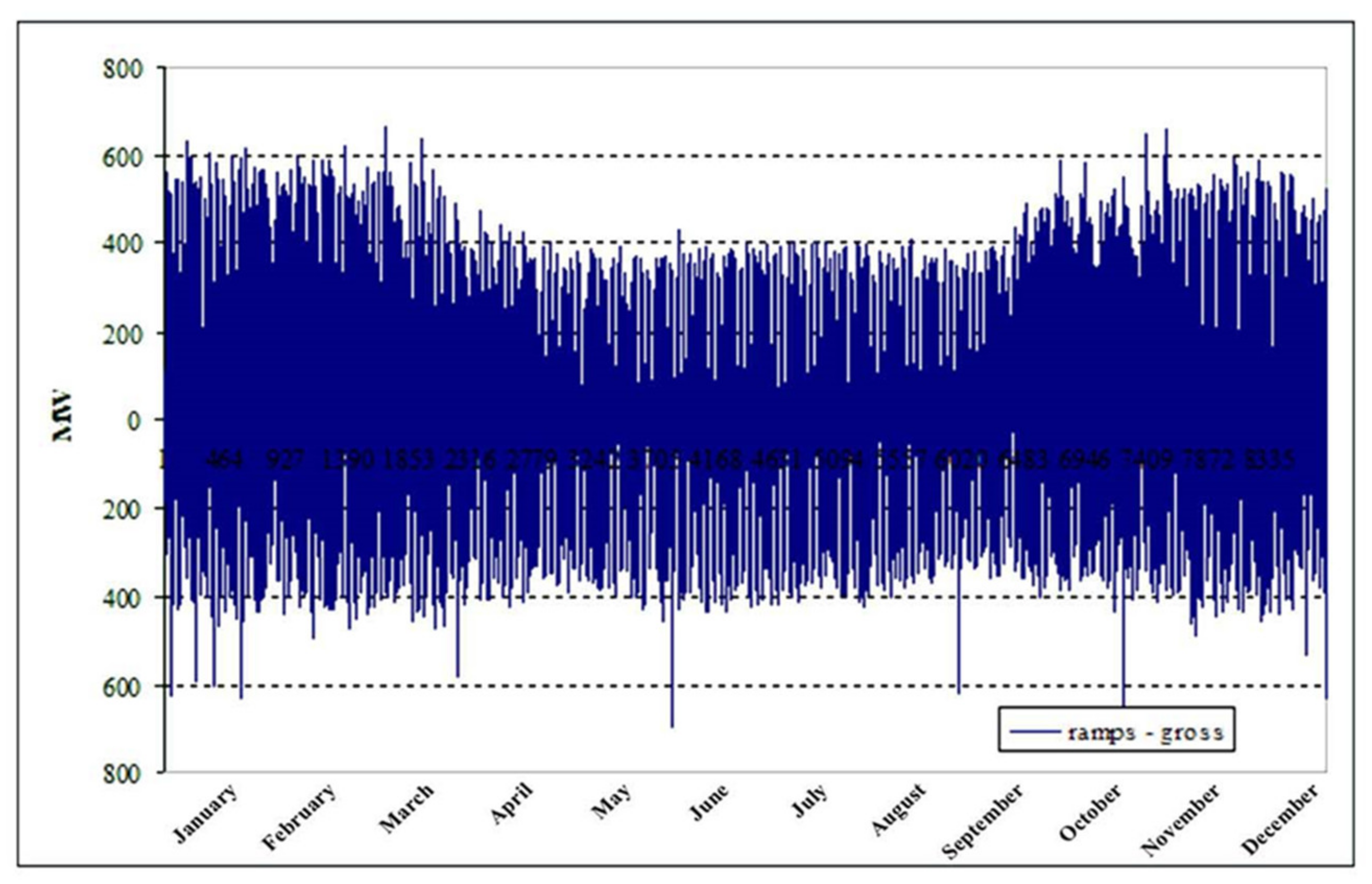
• Calculation of hourly ramps of gross load and residual load

The hourly ramps of any time series are defined as the differences between two consecutive hourly values of the process. In the case of gross load and residual load the hourly ramps are calculated as follows:

$$d{P}_{gross, i}=P_{gross,i}-P_{gross,i-1},$$

(13)

$$d{P}_{gross, i}=P_{gross,i}-P_{gross,i-1},$$

(14)

The hourly ramps of gross load are shown on Figure 8 and the resulting cumulative distribution functions for different penetrations of wind and PV are shown on Figure 9.

Simulations of hourly generations of wind and PV have been done with the following trends of increase of both installed capacities are shown in

Table 10. Trend of increase of installed capacities.

Increase, %	Wind, MW	PV, MW
0%	700	1040
25%	875	1300
50%	1050	1560
75%	1225	1820
100%	1400	2080

:

The resulting expectations (Mx) and standard deviations (σx) of the residual load for the above five cases and the case without RES (renewable energy sources—wind + PV) are as follows in

Table 11. Change of resulting indicators with the increase of total installed capacity of RES.

	No RES	Now RES	RES + 25%	RES + 50%	RES + 75%	RES + 100%
Mx MW	0	0	0	0	0	0
σx MW	212	218	224	231	239	248

:

Mathematical result expectation from the model may be positive or negative, being zero indicates that the mathematical model is good.

The probability distribution functions (PDF) and the cumulative distribution functions (CDF) for the 6 cases are shown on Figure 10.

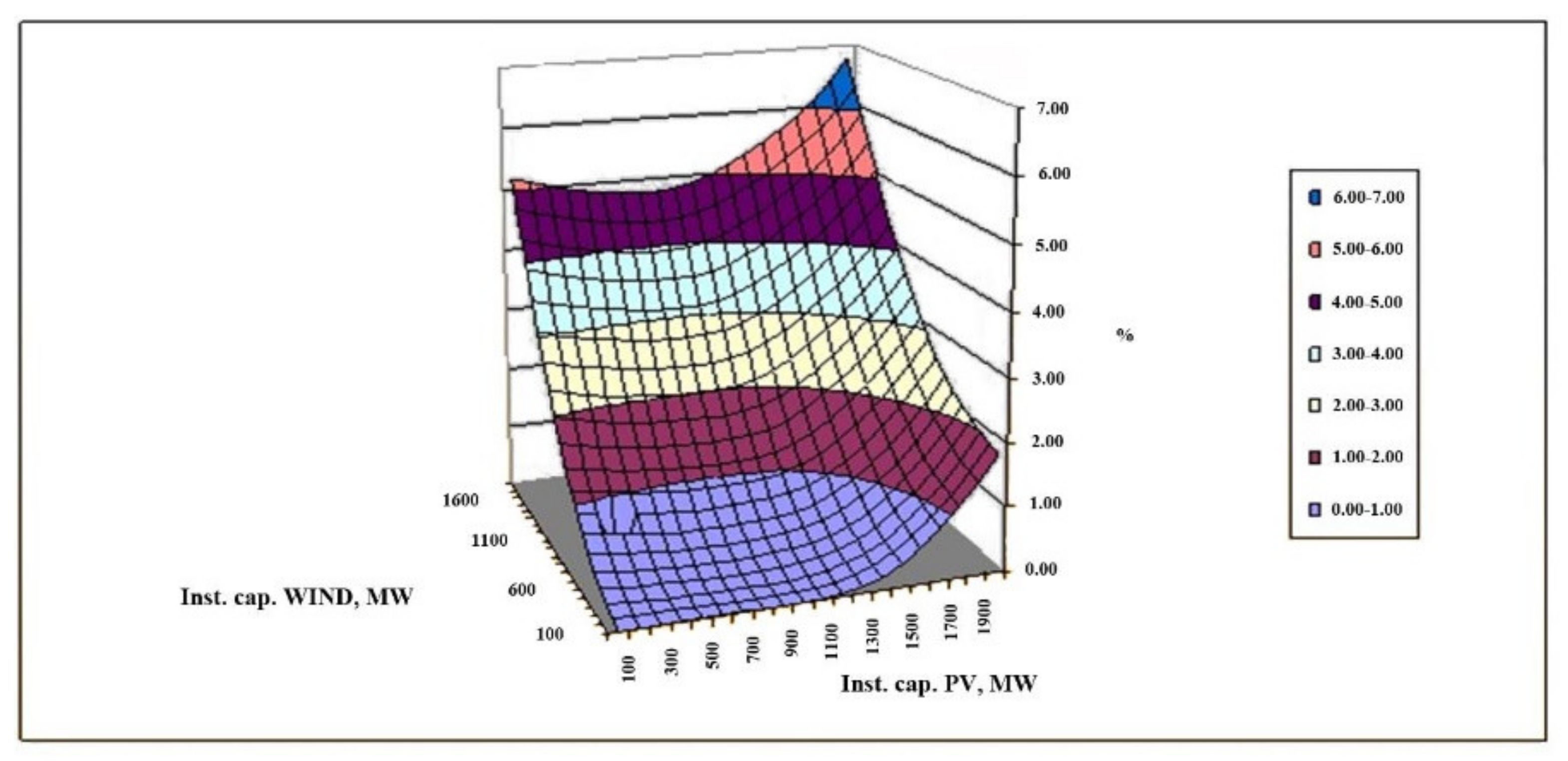
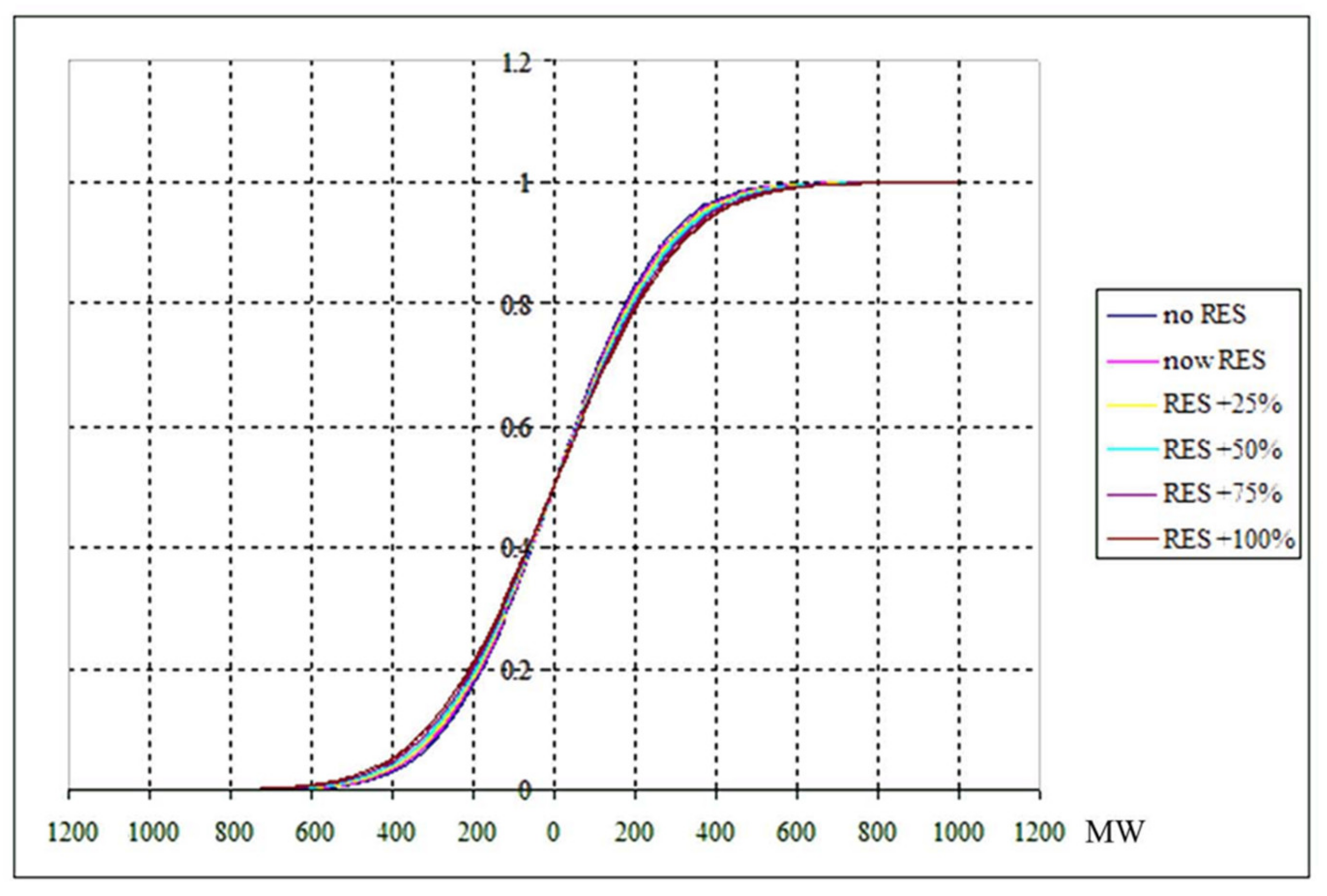
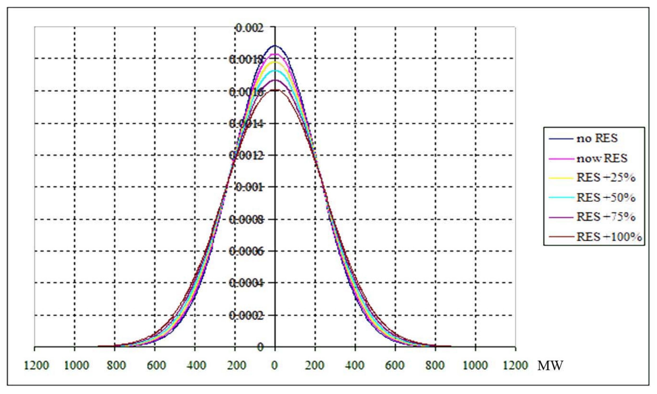
• Increasing the share of RES increases the capacity needed to cover the fluctuations in the electricity generated by RES.
• We are currently using 212 MW to cover RES deviations. With a 100% increase of RES we need to add an additional 36 MW of compensating power plants.

The linear regression model of the dependency of the standard deviation of the residual load hourly ramps from the installed capacities of WIND and PV was calculated using a multiple regression algorithm: The resulting model is as follows:

$${\sigma }_{residual load}=-538+0.50\ast WIN{D}_{cap}-0.13\ast P{V}_{cap},$$

(15)

where $WIN{D}_{cap}$—installed wind capacity and $P{V}_{cap}$—installed PV capacity.

This model can be used for calculating the standard deviation of hourly ramps of the residual load for any penetration of WIND and PV capacities.

The operational features of conventional units in BG power system are shown in

Table 12. Thermal power plants (coal).

Power Plant	Unit №	Pins, MW	Pmin, MW	Pmax, MW	Ramp Rate, MW/min	Time to Ramp from Pmin to Pmax, min
TPP MI 1 AES Galabovo	1	345	150	343	4	48
	2	345	150	343	4	48
TPP MI 2	1	177	135	172	1.5	25
	2	162	135	157	1.5	15
	3	172	135	167	1.5	21
	4	172	135	172	1.5	25
	5	225	155	222	2	34
	6	225	155	222	2	34
	7	227	155	225	2	35
	8	227	155	225	2	35
TPP MI 3 Contour Global	1	227	147	227	2.7	30
	2	227	147	227	2.7	30
	3	227	147	227	2.7	30
	4	227	147	227	2.7	30
TPP Bobod dol	1	190	140	190	3	17
	2	190	140	190	3	17
	3	190	140	190	3	17
TPP Maritsa 3	1	100	85	100	0.8	19
TPP Ruse	1	100	85	100	0.8	19
TPP Varna	1	210	110	210	3	33
	2	210	110	210	3	33
	3	210	110	210	3	33

.

The dependency of the total 1 min ramp rate (MW/min) from the on-line capacity of thermal units is calculated as well as dependency of total 15 min ramp rate. For hydro units the total 1 min ramp rate is calculated as well as the total 5 min ramp rate of hydro units.

The most common metrics used to quantify the available ramp resource of the conventional generation in a power system is the index called Insufficient Ramp Resource Probability—IRRP. R is is the probability that a system will not have sufficient ramping capability in a given direction over a year. Therefore, the IRRP needs to be specified over different time intervals and in both the positive and negative direction. So the reliability of a power system with respect to ramping is measured by IRRP.

The total ramp rates for different time interval—1 min, 15 min and 30 min of all thermal and hydro units is shown in Figure 11.

The extreme total hourly generations of thermal and hydro units in BG power system (2017 data) are estimated as follows: minimum hourly generation 1350 MW and maximum 5400 MW. The corresponding to 1350 MW online capacity value of total ramp rate for 30 min interval is 420 MW. Using the cumulative distribution functions of hourly ramps of the residual load for different penetrations of wind and PV (Figure 11), the following values of IRRP are calculated and presented in

Table 13. Resulting values of IRRP with the increase of RES installed capacity.

No RES	Now RES	RES + 25%	RES + 50%	RES + 75%	RES + 100%
0.0239	0.0272	0.0305	0.0347	0.0396	0.0453

below:

The corresponding to 5400 MW online capacity value of total ramp rate for 30 min interval is 2530 MW. For this value for all 6 cases the IRRP is equal to 0. Following the CDF’s of all six cases and values of total ramp rates (30 min) the online capacities above which the resulting IRRP are equal to zero were calculated. These capacities are as follows in

Table 14. Online capacities above which the resulting IRRP are equal to zero.

No RES	Now RES	RES + 25%	RES + 50%	RES + 75%	RES + 100%
2640	2667	2724	2793	2860	2930

:

The number of hours in the year with IRRP = 0 by referent cases is given in

Table 15. The number of hours in the year with IRRP = 0 with the increase of RES installed capacity.

No RES	Now RES	RES + 25%	RES + 50%	RES + 75%	RES + 100%
2640	2667	2724	2793	2860	2930

:

For all remaining hours IRRP is in the following intervals presented in

Table 16. The number of hours in the year with IRRP=0 with the increase of RES installed capacity.

Power Plant	Unit №	Pins, MW	Pmin, MW	Pmax, MW	Ramp Rate, MW/min	Time to Ramp from Pmin to Pmax, min
PSHPP Chaira	1	216	130	216	8	11
	2	216	130	216	8	11
	3	216	130	216	8	11
	4	216	130	216	8	11
PSHPP Belmeken	1	75	5.2	72	3.6	19
	2	75	5.2	72	3.6	19
	3	75	5.2	72	3.6	19
	4	75	5.2	72	3.6	19
	5	75	5.2	72	3.6	19
HPP Sestrimo	1	120	15	120	17.5	6
	2	120	15	120	17.5	6
HPP Momina klisura	1	61	22.5	61	3	13
	2	61	22.5	61	3	13
HPP Batak	1	11.7	1	11.2	4	3
	2	11.7	1	11.2	4	3
	3	11.7	1	11.2	4	3
	4	11.7	1	11.2	4	3
HPP Peshtera	1	27	1	21.6	6.4	3
	2	27	1	21.6	6.4	3
	3	27	1	21.6	6.4	3
	4	27	1	21.6	6.4	3
	5	27	1	21.6	6.4	3
HPP Aleko	1	23.7	4.3	23.7	2.7	7
	2	23.7	4.3	23.7	2.7	7
	3	23.7	4.3	23.7	2.7	7
HPP Teshel	1	30	6	30	1.5	16
	2	30	6	30	1.5	16
HPP Devin	1	44	18	41	1.5	15
	2	44	18	41	1.5	15
HPP Tsankov kamak	1	43.8	18	43.8	3	9
	2	43.8	18	43.8	3	9
PSHPP Orfei	1	40	5	40	4	9
	2	40	5	40	4	9
	3	40	5	40	4	9
	4	40	5	40	4	9
HPP Kritchim	1	41	15	41	4	7
	2	41	15	41	4	7
HPP Kardzhali	1	31	10	27.5	5.2	3
	2	31	10	27.5	5.2	3
	3	31	10	27.5	5.2	3
	4	31	10	27.5	5.2	3
HPP Studen kladenec	1	16.8	1	16.8	4.2	4
	2	16.8	1	16.8	4.2	4
	3	16.8	1	16.8	4.2	4
	4	16.8	1	16.8	4.2	4
	5	18	3	18	4.2	4
HPP Ivailovgrad	1	38	5	38	3	11
	2	38	5	38	3	11
	3	38	5	38	3	11

:

The number of hours with residual load being lower than the minimum must-run capacity of thermal coal plants are calculated for two options; 600 MW must-run capacity and 1000 MW must-run capacity. The results are as follows in

Table 17. Change of two important indicators with the increase of installed capacities of wind and PV plants.

Increase, %	Wind, MW	PV. MW	Number of Hours with Residual Load < 600 MW	Number of Hours with Residual Load < 1000 MW
0%	700	1040	66	259
25%	875	1300	123	336
50%	1050	1560	169	436
75%	1225	1820	236	542
100%	1400	2080	343	676

:

The location of hours with residual load below 1000 MW for case 6 (wind = 1400 MW and PV = 2080 MW) is also calculated. It is observed that most of the hours are in April when PV generation is higher due to climatic conditions and at the same time the demand is relatively low—this being the comfort period regarding daily average temperatures when neither heating nor cooling demand is needed. For these hours curtailment of wind and PV is needed in order to balance the system and this is identified as a downward regulation problem.

4. Conclusions

The presented approach for quantifying the influence of RES penetration on flexibility requirements has been applied for planning purposes in the Bulgarian power system.

• Examination of two estimated scenarios for 2021 electricity mix shows that with a difference in RES penetration of 10%, difference in demand of 25% and decrease in net exports by 50% (related with RES penetration increase in the adjacent countries), (i) the number of hours of in the year in which the residual load is lower than the absolute minimum annual gross total load will increase approximately 8 times and (ii) number of hours in the year in which the residual load is lower than the corresponding minimum admissible generation will increase approximately 4 times;
• The aforementioned results together with the coal units’ phase out program even before 2022 and the lack of big industrial loads, lead the TSO of Bulgaria to the estimation that further future integration of RES in the years beyond 2021 will result in balancing problems;
• The fast increase in installed RES will cause big sudden changes in balancing the ‘generation- consumption’ of Bulgarian EES. With insufficient regulating capacities, it will hamper the completion of the energy exchange schedules with neighboring EES;
• Installed RES plants are unable to provide the system operator with ancillary services (primary and secondary frequency regulation and capacity exchange) and cannot participate in the anti-emergency management of EES and recovering EES after heavy damage. SPP cannot participate in covering maximum winter loads, which are around 19–21 PM, and WPP produce the most electrical energy between 02–06 AM, when the consumption is minimal and there is excess energy in the grid.

This paper has presented a probabilistic approach for flexibility assessment in a power system based on the calculation of a set of seven indicators which quantify the impact of RES penetration based on the comparison between the net and the residual load statistical properties. The proposed approach can be used to predict the requirements for generation flexibility according to the expected scenario of RES penetration in the future development of EES and specially in a ten-year development plan and can be used for further probabilistic assessment of additional flexibility resources of system flexibility—interconnection capacity, hydro power plants, demand response etc.

We have proven that the large amount of RES is a serious problem when regulation towards the opposite direction (down) is needed. In this case it is important to turn on additional consumers which at the present moment is achieved by using pumps for load regulation. This possibility for the country has already been exhausted. Bulgaria does not have possibilities for down regulation, and when additional RES are included, the situation deteriorates. The new RES causes big and sudden changes in the generation-consumption balance and in the absence of regulating capacity, the electricity exchange schedules with the neighboring EESs are hampered. This leads to a violation of the quality of secondary regulation adopted by the countries from Continental Europe.

Further work will include the assessment of two and three hour ramps of the residual load in order to catch extreme variations in wind generation during massive weather fronts with high gradients of weather conditions We plan to use similar approach to differentiate between expected energy not served (ENS) due to inadequate capacity, and ENS due to inadequate flexibility.

References

1. Nosair, H.; Bouffard, F. Flexibility Envelopes for Power System Operational Planning. IEEE Trans. Sustain. Energy 2015, 6, 800–809. [Google Scholar] [CrossRef] [Green Version]
2. Ulbig, A.; Andersson, G. Analyzing operational flexibility of electric power systems. Int. J. Electr. Power Energy Syst. 2015, 72, 155–164. [Google Scholar] [CrossRef]
3. Lannoye, E.; Flynn, D.; O’Malley, M. Transmission, variable generation, and power system flexibility. IEEE Trans. Power Syst. 2015, 30, 57–66. [Google Scholar] [CrossRef]
4. Yang, J.; Zhang, L.; Han, X.; Wang, M. Evaluation of operational flexibility for power system with energy storage. In Proceedings of the 2016 International Conference on Smart Grid and Clean Energy Technologies (ICSGCE), Chengdu, China, 19–22 October 2016; pp. 187–191. [Google Scholar]
5. Bucher, M.A.; Chatzivasileiadis, S.; Andersson, G. Managing Flexibility in Multi-Area Power Systems. IEEE Trans. Power Syst. 2016, 31, 1218–1226. [Google Scholar] [CrossRef] [Green Version]
6. Capasso, A.; Falvo, M.C.; Lamedica, R.; Lauria, S.; Scalcino, S. A new methodology for power systems flexibility evaluation. IEEE Russia Power Tech. 2005, 1–6. [Google Scholar] [CrossRef]
7. European Commission. Clean Energy for All Europeans: Communication from the Commission to the European Parliament, the Council, the European Economic and Social Committee, the Committee of the Regions and the European Investment Bank. 2016. Available online: https://eur-lex.europa.eu/legal-content/PL/TXT/?uri=CELEX:52016DC0860 (accessed on 20 November 2019).
8. Molitor, C.; Monti, A.; Moser, A. Residential City Districts as Flexibility Resource: Analysis, Simulation and Decentralized Coordination Algorithms; RWTH Aachen University: Aachen, Germany, 2015. [Google Scholar]
9. Dall’Anese, E.; Mancarella, P.; Monti, A. Unlocking Flexibility: Integrated Optimization and Control of Multienergy Systems. IEEE Power Energy Mag. 2017, 15, 43–52. [Google Scholar] [CrossRef]
10. Wang, Q.; Hodge, B.M. Enhancing power system operational flexibility with flexible ramping products: A review. IEEE Trans. Ind. Inform. 2017, 13, 1652–1664. [Google Scholar] [CrossRef]
11. Yasuda, Y.; Årdal, A.R.; Huertas-Hernando, D.; Carlini, E.M.; Estanqueiro, A.; Flynn, D.; Gomez-Lazaro, E.; Holttinen, H.; Kiviluoma, J.; Van Hulle, F.; et al. Flexibility chart: Evaluation on diversity of flexibility in various areas. In Proceedings of the 12th International Workshop on Large-Scale Integration of Wind Power into Power Systems as well as on Transmission Networks for Offshore Wind Farms, WIW13, London, UK, 22–24 October 2013. [Google Scholar]
12. Cochran, J.; Miller, M.; Zinaman, O.; Milligan, M.; Arent, D.; Palmintier, B.; O’Malley, M.; Mueller, S.; Lannoye, E.; Tuohy, A.; et al. Flexibility in 21st Century Power Systems. 21st Century Power Partnership; National Renewable Energy Lab. (NREL): Golden, CO, USA, 2014; p. 14. [Google Scholar]
13. Lannoye, E.; Flynn, D.; O’Malley, M. Evaluation of power system flexibility. IEEE Trans. Power Syst. 2012, 27, 922–931. [Google Scholar] [CrossRef]
14. Ma, J.; Silva, V.; Belhomme, R.; Kirschen, D.S.; Ochoa, L.F. Exploring the use of flexibility indices in low carbon power systems. In Proceedings of the 3rd IEEE PES Innovative Smart Grid Technologies Europe (ISGT Europe), Berlin, Germany, 14–17 October 2012; pp. 1–5. [Google Scholar]
15. Thatte, A.A.; Sun, X.A.; Xie, L. Robust optimization based economic dispatch for managing system ramp requirement. In Proceedings of the Annual Hawaii International International Conference on Systems Science, Waikoloa, HI, USA, 6–9 January 2014; pp. 2344–2352. [Google Scholar]
16. Vita, V.; Zafiropoulos, E.; Gonos, I.F.; Mladenov, V.; Chobanov, V. Power system studies in the clean energy era: From capacity to flexibility adequacy through research and innovation. In Proceedings of the 21st International Symposium on High Voltage Engineering (ISH 2019), Budapest, Hungary, 26–30 August 2019. [Google Scholar] [CrossRef] [Green Version]
17. Bucher, M.A.; Delikaraoglou, S.; Heussen, K.; Pinson, P.; Andersson, G. On Quantification of Flexibility in Power Systems. In Proceedings of the PowerTech Eindhoven 2015 IEEE, Eindhoven, The Netherlands, 29 June–2 July 2015. [Google Scholar] [CrossRef] [Green Version]
18. Abujarad, S.Y.; Mustafa, M.W.; Jamian, J.J.; Abdilahi, A.M. Flexibility quantification for thermal power generators using deterministic metric for high renewable energy penetration. In Proceedings of the 2016 IEEE International Conference on Power and Energy (PECon), Melaka, Malaysia, 28–29 November 2016; pp. 580–584. [Google Scholar] [CrossRef]
19. Mladenov, V.; Chobanov, V.; Zafeiropoulos, E.; Vita, V. Characterisation and evaluation of flexibility of electrical power system. In Proceedings of the 10th Electrical Engineering Faculty Conference (BulEF), Sozopol, Bulgaria, 11–14 September 2018. [Google Scholar] [CrossRef]
20. Seritan, G.; Porumb, R.; Grigorescu, S.; Pagano, M. Statistical analysis on wind variability impact on environment. In Proceedings of the 8th International Conference on Modern Power Systems (MPS), Cluj Napoca, Romania, 21–23 May 2019; pp. 1–6, WOS000612401900007. [Google Scholar]
21. Ceaki, O.; RVatu Golovanov, N.; Porumb, R.; Serițan, G. Analysis of the Grid-Connected PV Plants Behavior with FACTS Influence. In Proceedings of the UPEC 2014, 49th International Universities’ Power Engineering Conference, Cluj-Napoca, Romania, 2–5 September 2014; pp. 1–6, ISBN 978-1-4799-6556-4. [Google Scholar] [CrossRef]
22. Mladenov, V.; Chobanov, V.; Zafeiropoulos, E.; Vita, V. Flexibility assessment studies worldwide-bridging with the adequacy needs. In Proceedings of the 11th Electrical Engineering Faculty Conference (BulEF), Varna, Bulgaria, 11–14 September 2019. [Google Scholar] [CrossRef]
23. International Energy Agency. Harnessing Variable Renewables: A Guide to the Balancing Challenge; OECD Publishing: Paris, France, 2011. [Google Scholar]
24. Mladenov, V.; Chobanov, V.; Zafiropoulos, E.; Vita, V. Flexibility issues in EU, Bulgarian and Greek power networks. In Proceedings of the 2nd South East European Regional CIGRE Conference, Kyiv, Ukraine, 12–13 June 2018. [Google Scholar]
25. Hillberg, E. Flexibility Needs in the Future Power System; ISGAN Annex 6 Power T&D Systems; ISGAN: Washington, DC, USA, 2019. [Google Scholar]
26. Bouffard, F.; Ortega-Vazquez, M. The Value of Operational Flexibility in Power Systems with Significant Wind Power Generation. In Proceedings of the Power and Energy Society General Meeting, Detroit, MI, USA, 24–28 July 2011; pp. 1–5. [Google Scholar] [CrossRef]
27. Stratigakos, A.; Krommydas, K.; Papageorgiou, P.; Dikaiakos, C.; Papaioannou, G. A Suitable Flexibility Assessment Approach for the Pre-Screening Phase of Power System Planning Applied on the Greek Power System. In Proceedings of the IEEE EUROCON 2019—18th International Conference on Smart Technologies, Novi Sad, Serbia, 1–4 July 2019; pp. 1–6. [Google Scholar] [CrossRef]
28. Holttinen, H.; Tuohy, A.; Milligan, M.; Lannoye, E.; Silva, V.; Müller, S.; Sö, L. The flexibility workout: Managing variable resources and assessing the need for power system modification. IEEE Power Energy Mag. 2013, 11, 53–62. [Google Scholar] [CrossRef]
29. Dvorkin, Y.; Kirschen, D.S.; Ortega-Vazquez, M.A. Assessing flexibility requirements in power systems. IET Gener. Transm. Distrib. 2014, 8, 1820–1830. [Google Scholar] [CrossRef]
30. Makarov, Y.V.; Loutan, C.; Ma, J.; De Mello, P. Operational impacts of wind generation on California power systems. IEEE Trans. Power Syst. 2009, 24, 1039–1050. [Google Scholar] [CrossRef]
31. Ela, E.; Milligan, M.; Bloom, A.; Botterud, A.; Townsend, A.; Levin, T.; Frew, B.A. Wholesale electricity market design with increasing levels of renewable generation: Incentivizing flexibility in system operations. Electr. J. 2016, 29, 51–60. [Google Scholar] [CrossRef] [Green Version]
32. Witte, R.S.; Witte, J.S. Statistics, 11th ed.; John Wiley & Sons: Hoboken, NJ, USA, 2017; ISBN 978-1-119-25451-5. [Google Scholar]
Figure 1. Variation of the minimum admissible generation in the EPS of Bulgaria in hourly resolution during the year 2019.
Energies 14 02813 g001
Figure 2. Dependence of the potential generation curtailment in % of the total annual production from wind and PV on their installed capacity.
Energies 14 02813 g002
Figure 3. Model values of hourly generations of nuclear, CHP, biomass and run-off-river.
Energies 14 02813 g003
Figure 4. Expected average export.
Energies 14 02813 g004
Figure 5. Simulated wind hourly generations.
Energies 14 02813 g005
Figure 6. Simulated PV hourly generations.
Energies 14 02813 g006
Figure 7. Hourly values of gross load and resulting hourly values of residual load.
Energies 14 02813 g007
Figure 8. Hourly ramps of gross load.
Energies 14 02813 g008
Figure 9. Resulting cumulative distribution functions for different penetrations of wind and PV.
Energies 14 02813 g009
Figure 10. Resulting probability distribution functions for different penetrations of wind and PV.
Energies 14 02813 g010
Figure 11. Total available ramp rates from thermal and hydro units vs. total on-line ro capacity for different time intervals.
Energies 14 02813 g011