Quantification of Energy Flexibility and Survivability of All-Electric Buildings with Cost-Effective Battery Size: Methodology and Indexes

Abstract

All-electric buildings are playing an important role in the electrification plan towards energy-neutral smart cities. Batteries are key components in all-electric buildings that can help the demand-side energy management as a flexibility asset and improve the building survivability in the case of power outages as an active survivability asset. This paper introduces a novel methodology and indexes for determining cost-effective battery sizes. It also explores the possible trade-off between energy flexibility and the survivability of all-electric buildings. The introduced methodology uses IDA-ICE 4.8 as a building performance simulation tool and MATLAB^® 2017 as a post-processing calculation tool for quantifying building energy flexibility and survivability indexes. The proposed methodology is applied to a case study of a Norwegian single-family house, where 10 competitive designs, 16 uncertainty scenarios, and 3 dynamic pricing tariffs suggested by the Norwegian regulators are investigated. The methodology provides informative support for different stakeholders to compare various building designs and dynamic pricing tariffs from the flexibility and survivability points of view. Overall, the results indicate that larger cost-effective batteries usually have higher active survivability and lower energy flexibility from cost- effectiveness perspective. For instance, when the time of use tariff is applied, the cost-effective battery size varies between 40 and 65 kWh (daily storage). This is associated with a cost-effective flexibility index of 0.4–0.55%/kWh and an active survivability index of 63–80%.

1. Introduction

1.1. Building Electrification

Electrification of the energy use in the final sectors has been highlighted as an important pathway to decarbonizing energy systems [1]. In particular, the heating [2] and transport [3] sectors are receiving considerable attention in the electrification era. Heating demand accounts for a significant share of total energy use in the European building sector [4], providing the grounds for moving toward building electrification and all-electric buildings. Currently, some end uses, such as lighting, appliances, and refrigeration are already dominated by electricity in the building sector. All-electric buildings use electricity for other end uses, such as heating, domestic hot water, cooking, and cooling, that are usually powered by other sources of energy (e.g., fossil fuels). Heat pumps are one of the enabling technologies for widespread building electrification and their growing usage at the EU level and in general are highlighted by the European Heat Pump Association (EHPA) [5] and the International Energy Agency (IEA) [6], respectively. So, electrification of the building sector plays an important role in the decarbonization process along with the application of other strategies such as providing building demands from hydrogen, waste-heat reuse [7], combined heat and power (CHP), and district heating systems (DH). Implementation of renewable energy sources (RES) along with electrification will increase the share of clean and zero-carbon electricity in the grid during the operational phase. However, it should be noted that these energy sources actually consume a large amount of energy and emit emissions during their life cycle. Furthermore, energy production from renewable sources is intermittent [8], fluctuates [9], difficult to forecast [10], and requires strategies for balancing supply and demand [11]. In addition, electrification of residential heating and transportation can increase peak loads and require both greater generation and grid capacity [12]. Norway can be a good representative case for this condition. Norwegian power production is largely dominated by hydropower (95%) [13], and the electricity generated from hydropower is the main energy source for Norwegian dwellings. The availability of relatively cheap electricity has increased the usage of electric-based heating systems [14], the share of electric vehicles, and so on. For instance, 63.1% of the space heating and 96.2% of the domestic hot water (DHW) in Norway are produced by electricity [15]. Furthermore, Norway remained the global leader in terms of electric car market share at 56% of its new car sales in 2019, more than double the second-largest market share in Iceland at 22% [16].

1.2. Demand Response

Demand-response (DR) programs can be used to decrease the fluctuation in energy production via renewable sources, fully utilize the generated energy, and balance the power grid and relieve it during peak loads [17]. Different techniques, such as peak shaving, load shifting, valley filling, and minimizing curtailment time, can modulate building load in DR programs [18]. These programs are generally categorized into two groups [19]: incentive-based DR programs, where economic incentives are provided by utilities, load serving entities, or a regional grid operator in order to decrease customer demand during a capacity shortage or times of high electricity prices, and price-based DR programs, where customers change their normal electricity usage patterns in response to dynamic pricing tariffs. Both of these approaches have their own advantages and drawbacks [20]. Dynamic pricing tariffs are one of the most important DR programs and encourage users to consume more wisely and efficiently. They utilize different schemes, such as time of year (seasonal) pricing, time of use pricing (daily or weekly), critical-peak pricing, and real-time pricing [21]. There are some studies in the literature that have simulated households’ behaviors under time-based prices [22]. Achieving energy efficient, renewably based, smart, and flexible buildings is one of the goals of the European Green Deal, which focuses on full decarbonization by 2050 [23].

1.3. Energy Flexibility

Application of DR programs can lead to adjustments in power system supply and demand, which is known as flexibility [24]. Flexible loads in residential buildings are related to household appliances (e.g., washing machines and dishwashers), electric vehicles, and space or water heating systems. There are survey-based studies that have shown that participants are willing to shift their white goods loads as flexible loads when it comes to variable pricing schemes [25]. Laicane et al. investigated the potential of demand side management with assessing load shifts in the washing machine and dishwasher usage and showed that these load shifts can decrease the dwelling peak load by 24% and 13.5%, respectively [26]. The participation of electric vehicles in the price-based DR programs in commercial, industrial, and residential areas is studied in [27], which concludes that there is a good efficiency in the reduction of electricity use when price-based demand response is used in combination with electric vehicles (EVs). Moreau evaluated the load shift for water heaters and proposed a control strategy in order to minimize the peak load at the end of shifting time [28]. In [29], Mancini and Nastasi evaluated the impact of energy retrofitting on the energy flexibility of dwellings in a scenario, which is focusing on greater electrification of consumption. They concluded that electrified systems are facing a considerable increase in flexible loads in comparison to the gas-fed systems. Achieving flexibility in residential buildings is generally possible when storage systems are used as flexibility assets, depending on the energy system and types of DR programs [30]. Storage systems are categorized as electrical (e.g., batteries), active thermal, or passive thermal storage. These systems can be utilized as stand-alone storage systems or coupled with other technologies, such as heat pumps and combined heat and power systems (CHPs) [31,32]. Within the electrical storage category, battery storage is usually considered to be a flexibility asset with a time step of several hours, during which it can shift energy consumption from high-tariff to low-tariff periods or reduce the peak demand. Battery storage systems are modular and allow a wide range of applications. The falling cost of batteries and their combination with hybrid systems has made them an attractive storage option for homeowners [33]. A variety of optimization efforts in terms of sizing battery storage in combination with renewable energy sources have been undertaken for buildings [34,35,36,37]. For instance, Dmount et al. evaluated the integration of battery storage in a positive energy building equipped with energy systems, such as heat pumps and photovoltaic (PV) systems [38]. In addition, [39] implemented battery storage in combination with dynamic pricing tariffs in order to establish a dynamic interaction between the building and smart grid. Furthermore, it has been shown that batteries have great potential in terms of providing power for customers during power outages [40,41]. For instance, Tsianikas et al. [42] investigated optimized grid-outage resilient PV and battery systems from an economic point of view. The survivability of a solar energy system with local storage in the presence of a power outage was investigated in [43]. In this work, a certain percentage of battery capacity was reserved in case of a power outage. However, most studies on using batteries to achieve building survivability and resilience have focused on combinations of batteries (as storage systems) and renewable energy sources [44]. When put together, the above literature on building energy flexibility and survivability provides important insights into the application of batteries as “flexibility assets” for harnessing building energy flexibility and as “backup storage” for improving building survivability in the case of power outages. Furthermore, battery capacity can play an important role in the quantification of energy flexibility and survivability. However, far too little attention has been paid to the energy flexibility and survivability trade-off from a cost-effectiveness perspective.

1.4. Innovative Contributions

The aim of this work is to propose a methodology for exploring the trade-off between energy flexibility and survivability in all-electric buildings from a cost-effectiveness perspective in the context of dynamic pricing tariffs.The main contributions of this paper can be expressed as:

• Load shift calculation of electric-based heating demand in response to different business models for dynamic pricing tariffs.
• Formulation of a model to determine the cost-effective battery size needed for storing the shifted load.
• Introduction of the concept of “active survivability” in the context of all-electric buildings.
• Introduction of new flexibility and survivability indexes for the comparison of the possible designs for an all-electric building under different dynamic pricing tariffs.

These contributions have been achieved by developing a MATLAB-based algorithm. Two new indicators, the Cost-Effective Flexibility Index (CEFI) and Active Survivability Index (ASI), are introduced along with the proposed methodology. The CEFI allows the identification of energy flexibility in response to dynamic pricing tariff, and the ASI indicates the survivability of a building in the case of a power outage from an economical point of view. The CEFI and ASI generally depend on cost-effective sizes for the batteries selected for storing the heat shift and can be used in the case of power outages as backup storage. Furthermore, a set of designs known as competitive designs are implemented in this paper to allow comparisons of the energy flexibility and survivability of building designs with the same energy targets. In addition, uncertainties in building operation and external conditions can have an impact on the energy flexibility and survivability of building designs under different dynamic pricing tariffs. For this reason, weather and occupant scenarios are created to gauge the impact of these uncertainties on energy flexibility and survivability under different dynamic pricing tariffs. Indeed, the main novelty of this work is the exploration of the trade-off between the energy flexibility and survivability of all-electric buildings, potentially opening the door to more complex concepts such as energy-resilient buildings. Furthermore, the algorithm developed in this paper can be adjusted for different dynamic pricing tariffs at the country, city, or neighborhood level and can be used for all-electric buildings, which represent a growing trend (both in heating-dominated building in cold climates and cooling-dominated buildings in hot climates). Different stakeholders in the grid markets, such as policy makers, grid companies, building designers, and homeowners, can take advantage of this algorithm to evaluate the performances of buildings from flexibility and survivability perspectives with two easy-to-understand indicators.

To achieve the above mentioned goals, three different business models of dynamic pricing tariffs suggested by the Norwegian regulators are considered, along with ten different building designs with the same energy target for an all-electric Norwegian single-family house. In order to investigate the impacts of uncertainties on energy flexibility and survivability, 16 scenarios (eight occupant scenarios × two weather scenarios) are proposed, and the impacts of these uncertainties on energy flexibility and survivability are evaluated. The paper proceeds as follows: Section 2 provides overviews of cost-effective battery sizing and the energy flexibility and survivability quantification method, along with the requirements for using it. In Section 3, the proposed method is investigated using a case study of an all-electric Norwegian single-family house involving detailed descriptions of 10 different building designs and 16 weather and occupant scenarios. The results of this case study are presented and discussed in Section 4. A summary of the methodology, along with the main conclusions, is presented in Section 5.

2. Methodology

In this section, we present the research methodology, including the study concept. This methodology combines building performance simulation (BPS) and an in-house algorithm developed in MATLAB. Figure 1 shows the conceptual framework of the study, which consists of three stages: algorithm input, algorithm development, and algorithm output. These parts will be described in the following subsections.

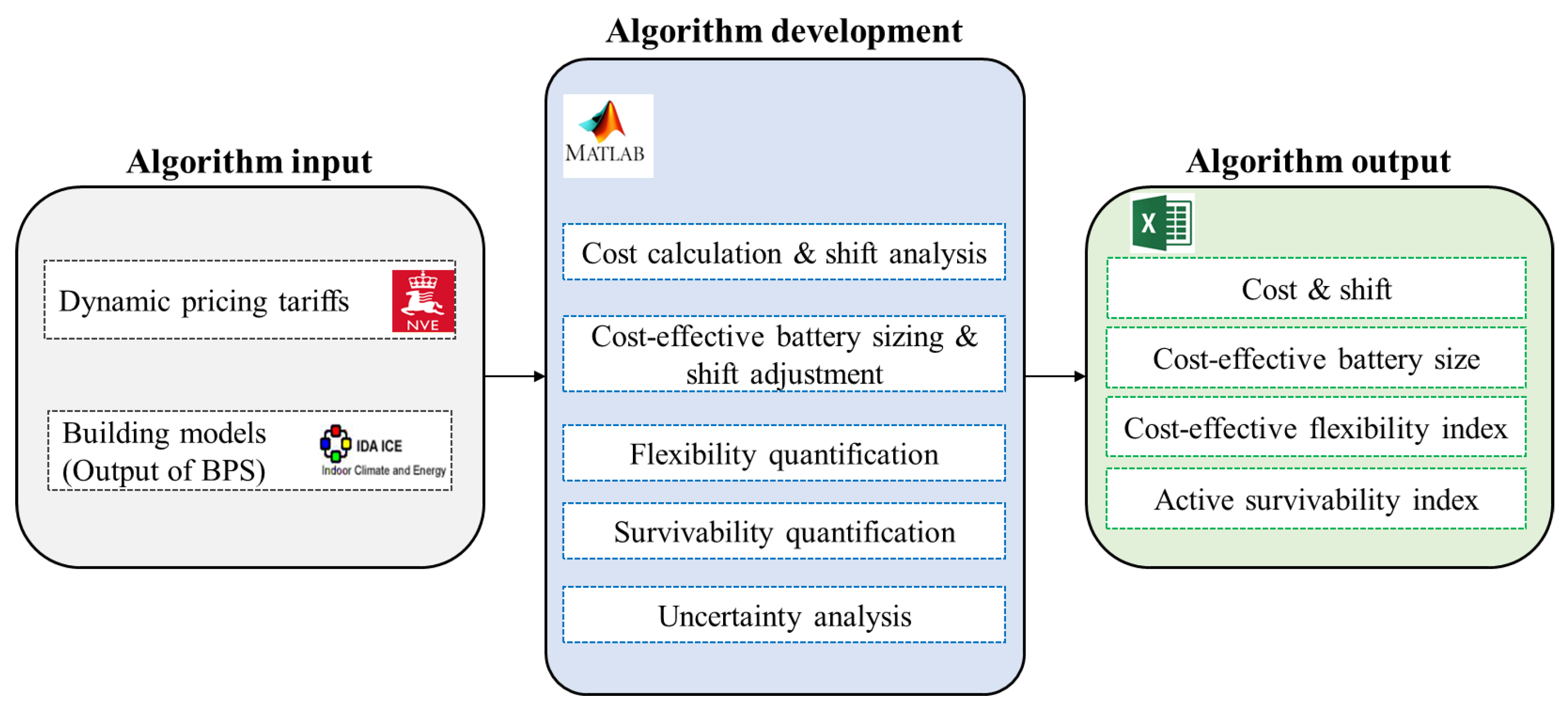
2.1. Algorithm Input

Different business models for the dynamic pricing tariffs and energy consumption resulted in building performance simulations are the required input data for the developed algorithm.

2.1.1. Business Models for Dynamic Pricing Tariffs in Norway

Today, Norwegian residential customers are faced with an energy-based grid rent tariff known as the “energy rate tariff model”, which consists of two parts: one fixed part and one volumetric part [45]. The fixed part is an annual cost that covers the costs associated with customer management and support and is the same for all customers. The volumetric part is an energy charge that is user-dependent and reflects energy consumption. This grid tariff does not differentiate between high and low power drains [46]. To solve this issue, dynamic pricing tariffs are recommended to incentivize better grid utilization [47]. Therefore, the Norwegian Water Resource and Energy Directorate (NVE) has proposed a new grid rent tariff to incentivize load shifts and peak load reductions in buildings [48]. The new tariff combines three different business models that allow for either higher costs during high-demand periods (time of use tariff), or higher costs for the power demands that exceed higher than a subscribed level (measured power rate tariff and tiered rate tariff). These tariffs will be illustrated in the following parts and Figure 2. It should be noted that the values presented for each tariff (

Table 1. Grid tariff rents for residential buildings in the energy rate tariff, measured power tariff, tiered rate tariff, and time of use tariff.

Energy Rate Tariff
Fixed cost	Energy cost	-	-
(€/year)	(€/kWh)
174.9	0.0194	-	-
Measured Power Rate Tariff
Fixed cost	Energy cost	Power cost	-
(€/year)	(€/kWh)	(€/kWh/h)
174.9	0.005	0.186	-
Tiered Rate Tariff
Fixed cost	Energy cost	Subscription cost	Overuse cost
(€/year)	(€/kWh)	(€/kWh/h)/year	(€/kWh/h)
174.9	0.005	68.9	0.1
Time of Use Tariff
Fixed cost	Summer energy cost	Winter day energy cost	Winter night energy cost
(€/year)	(€/kWh)	(€/kWh)	(€/kWh)
174.9	0.0122	0.038	0.0152

) are average numbers, which can vary between different distribution companies [46]. The other values related to taxes or levies are added to the grid rent tariff [49].

• Measured power rate tariff model.

This tariff consists of three different parts: a fixed part, an energy part, and a power part. The fixed part and the energy part are similar to parts in the energy rate tariff model, but the values can be changed. For instance, the value used in the energy part for the measured power rate tariff is less than that used in the energy rate tariff. The power part is determined based on the highest peak power outtake during the measurement period, and it is recommended that this part to be measured on a daily basis in the Norwegian regulations in order to match customer and grid peak demands [50]. However, for industrial customers, all of whom are using the measured power rate tariff currently, the highest peak period is measured on a monthly basis.

• Tiered rate tariff model.

This tariff consists of four different parts: a fixed part, a subscription limit, an energy part, and an overuse part. For this tariff, the customer subscribes to a capacity level (subscription limit), and, based on their violations of this level, a penalty (overuse part) is charged. In the short term, implementation of the penalty sends a price signal to the customer to reduce their consumption when it exceeds the subscription limit. On the other hand, in the long term, it helps customers to select a subscription limit leading to the lowest yearly costs. For most ordinary customers, the high and low power drains on the customer side are matched with high and low stress on the grid side, respectively. The overuse is applied to power drains above the limit, even when the grid has a good capacity. In this case, it will not create any benefits for the grid side. Furthermore, if the customer meets the subscription limit, he/she does not need to reduce his/her power drain, even when the grid is under high stress. These issues are the drawbacks of the tiered rate tariff model. In this study, we used an individual annual subscription that customers can select themselves or with help of grid distribution companies that cannot be changed over the course of a year. A Norwegian regulator sets a minimum usage of 1 kW but does not suggest exact power limits. This study considered ten limits. The appropriate power limit should be selected in this tariff to prevent high subscription or overuse costs.

• Time of use tariff model.

For this tariff, the electricity prices are set for specific time periods such as peak and off-peak hours. The peak hours are hours that have historically had high grid pressure, and the time of use tariff assigns higher energy prices to these hours. The time of use model suggested by the Norwegian regulator uses higher prices on winter days because they face grid stress [51]. Customers can understand this tariff easily because it differentiates pricing according to blocks of time and offers pricing terms of energy consumption (kWh) instead of power (kW), which is used in the two previous tariffs. The dependence of the pricing on blocks of time (two peak and off-peak blocks) makes this tariff rather unfit going forward with a higher penetration of intermittent generation unless it is coupled with other dynamic pricing strategies, such as critical peak pricing (CPP). Illustrations of the introduced tariffs for typical winter and summer days, along with the values for the different parts of each tariff, are provided in Figure 2 and Table 1, respectively.

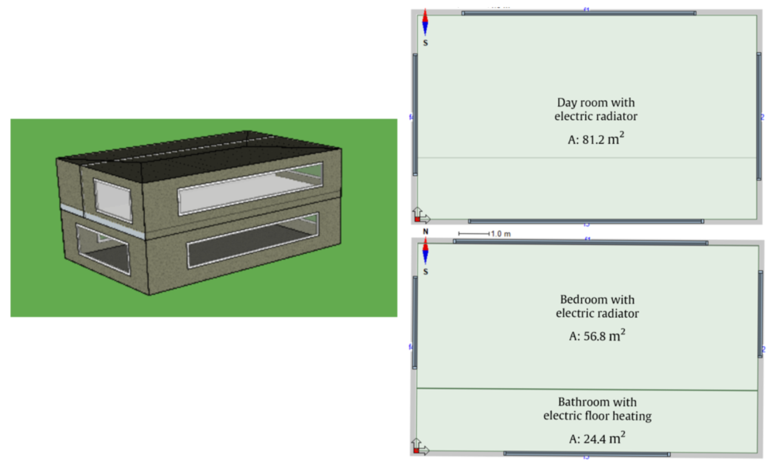
2.1.2. Building Models

Based on Figure 1, the building loads (including space heating, domestic hot water, etc.) are the second input of the developed algorithm. It is supposed that the building loads will be estimated in the early design phase using building performance simulation tools. The energy simulations for building models were conducted via the building performance simulation software IDA Indoor Climate and Energy (ICE), version 4.8 [52]. This dynamic, whole-building software applies equation-based modeling in Neutral Modeling Format (NMF) and has been validated using several validation tests [53,54]. A detailed dynamic of energy supply and system component can be simulated in this software, making it possible to evaluate the energy consumption and indoor climate of the building. In this study, the result of the simulation in IDA ICE was entered as an input to the developed algorithm to calculate the amount of shifted load and battery capacity and other parameters. The simulations were performed using a typical climate file (IWEC) from IDA ICE library [52].

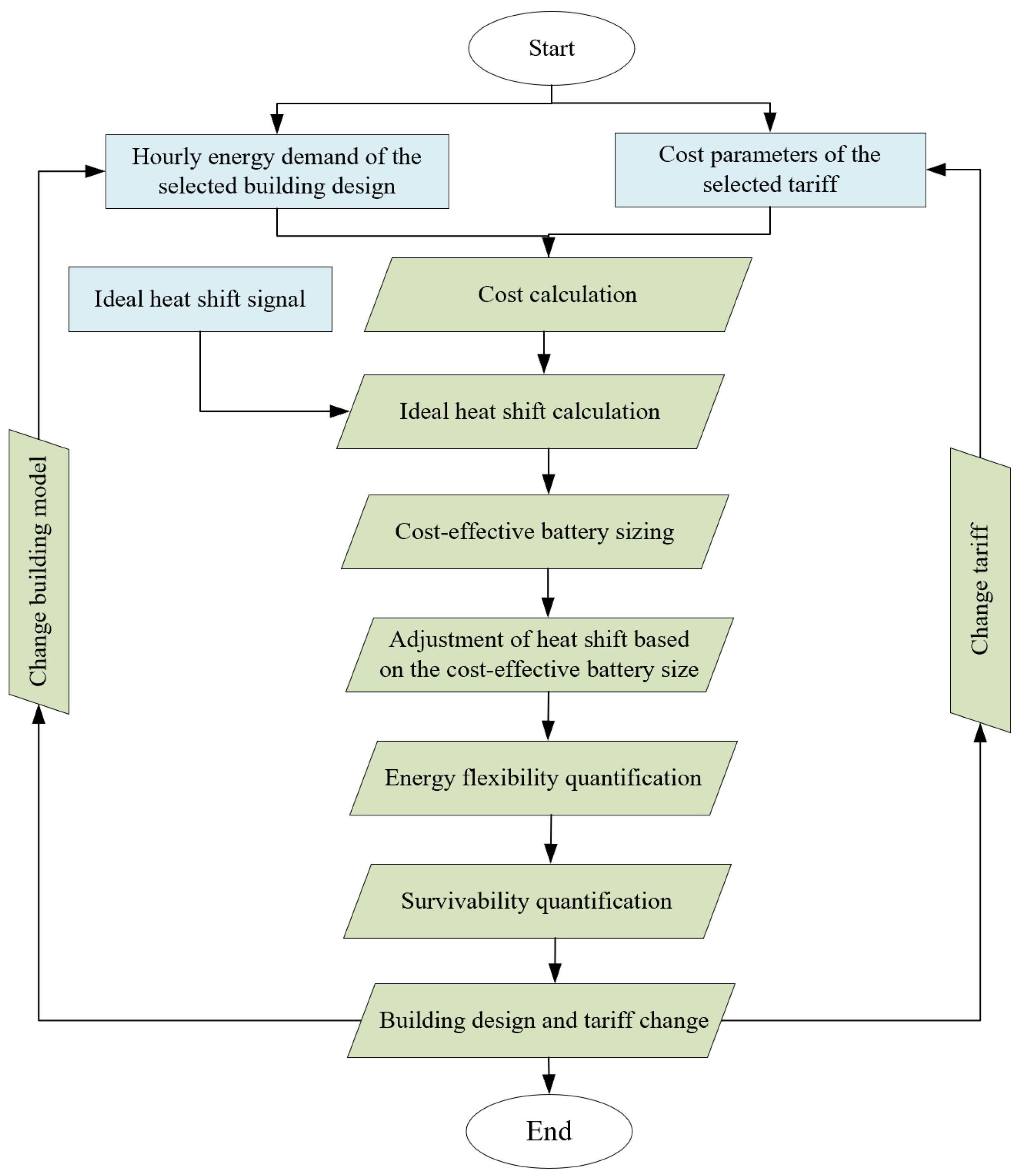
2.2. Algorithm Development

The developed algorithm in this paper is a MATLAB-based (MATLAB 2017 [55]) algorithm coupled with IDA ICE, which is based on a previous work done at the Norwegian University of Science and Technology [51]. While the previous work focused on an Excel-based algorithm for calculating the costs and ideal heat shifts for each business models of dynamic pricing tariffs, the current MATLAB-based algorithm adjusts the ideal shift based on the cost-effective battery size and adds a method for the quantification of energy flexibility and survivability of all-electric buildings. In the first step, the building design and tariff to be used are selected. After this step, the algorithm takes the hourly energy demand simulated for the building design in IDA ICE and computes the building’s energy costs under the selected tariff. After the cost calculation, the shifted load are calculated by implementing a signal referred to as the ideal heat shift signal (heat consists of electric-based space heating and the domestic hot water load), which is explained in more detail in Section 2.2.1. In the next step, the battery capacity for storing the shifted heat is determined based on the cost-effectiveness, producing the cost-effective battery size. The shift is then adjusted according to the cost-effective battery size. Thereafter, two new indexes are introduced for quantifying the energy flexibility and survivability of the building design under the selected tariff. In the last step, the building model and dynamic pricing tariff will be changed, and the procedure continues until all building models under all tariffs have been considered. The flow diagram for this procedure is shown in Figure 3 and is explained in more detail in the upcoming sections.

2.2.1. Cost Calculation and Shift Analysis

To calculate the energy costs of different building designs under the suggested business models for the dynamic pricing tariffs, the hourly energy demand taken from the building simulation (Section 2.1.2) and the values related to different parts of the dynamic pricing tariffs (Table 1) are entered as input data, and the cost calculation algorithm computes the costs of the different designs for each tariff.

Load shifting is one of the strategies that can be used with price-based DR programs. Flexible loads in the residential buildings can be categorized as belonging to household appliances, electric vehicles, space heating and cooling, and domestic hot water. Given the different business models for the dynamic pricing tariffs suggested by the Norwegian regulator, the electric-based heating load (consists of space heating and domestic hot water) is considered to be the shifted in this paper. This load has been selected for the following reasons: First, space heating and domestic hot water combine to form the largest share of a building’s energy consumption in countries with cold climates, such as Norway. Second, shifting other loads, such as household appliances loads, amounts to running them at night or when no one is home. This strategy will lead to lower energy costs, but it has disadvantages, such as the risk of fire [51]. Furthermore, the energy source for most Norwegian residential buildings is electricity. Therefore, we can focus on electric-based heat shifting without sacrificing thermal comfort and use batteries without including thermal storage. The proposed methodology can also be adjusted and used for shifting the cooling load in countries with hot climates. Based on the work of Karlsen et al. [51], the ideal heat shift is considered first in this paper. The ideal heat shift is a theoretical optimum amount of shift that leads to the lowest costs with respect to the implemented tariff [51]. In the next steps, the amount of this shift will be adjusted based on the cost-effective battery size that is selected for storing the shift. The assumptions for this ideal load shift are as follows:

• The ideal heat shift consists of the space heating and domestic hot water loads.
• The ideal heat shift will not sacrifice the occupant’s comfort (regarding space heating and domestic hot water).
• The storage of the shifted load is considered in a daily-based manner (kWh/day).
• No losses are considered during the ideal load shift.

The implementation of the ideal load shift for each of the suggested business models of the dynamic pricing tariff leads to specific load profiles and shift patterns for each tariff, which are shown in Figure 4. The following points should be considered regarding the shifting patterns in each business model for the dynamic pricing tariffs.

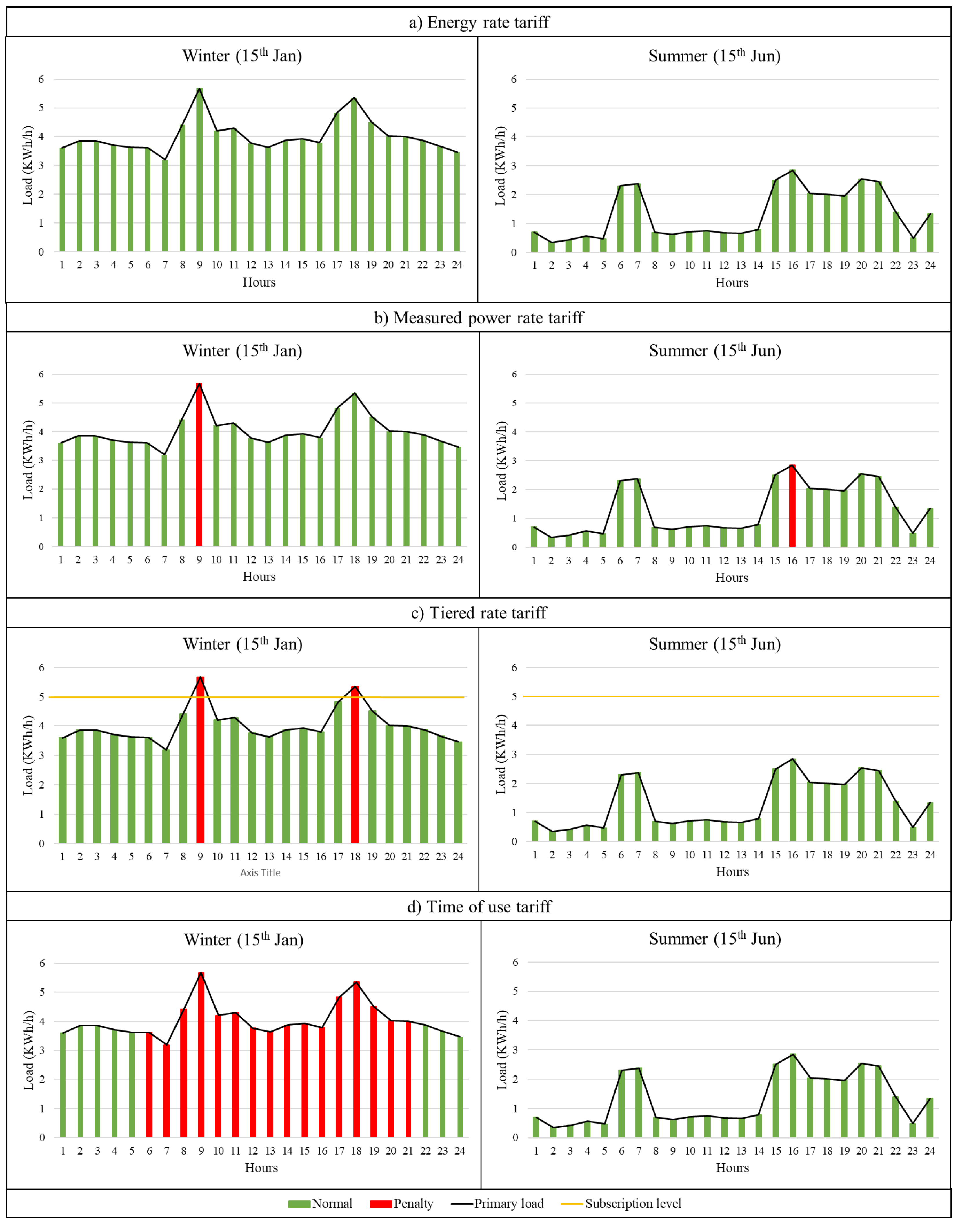
• The energy rate tariff applies the same energy price during all hours of the year, so load shifting under this tariff will not be beneficial from the customer’s point of view. Even though shifting can remove the stress from the grid in peak hours, no shifts will be implemented as long as they are not beneficial. In addition, no one will pay for the storage of the shifted load without receiving benefits. Hence, the load profile remains constant for the energy rate tariff.
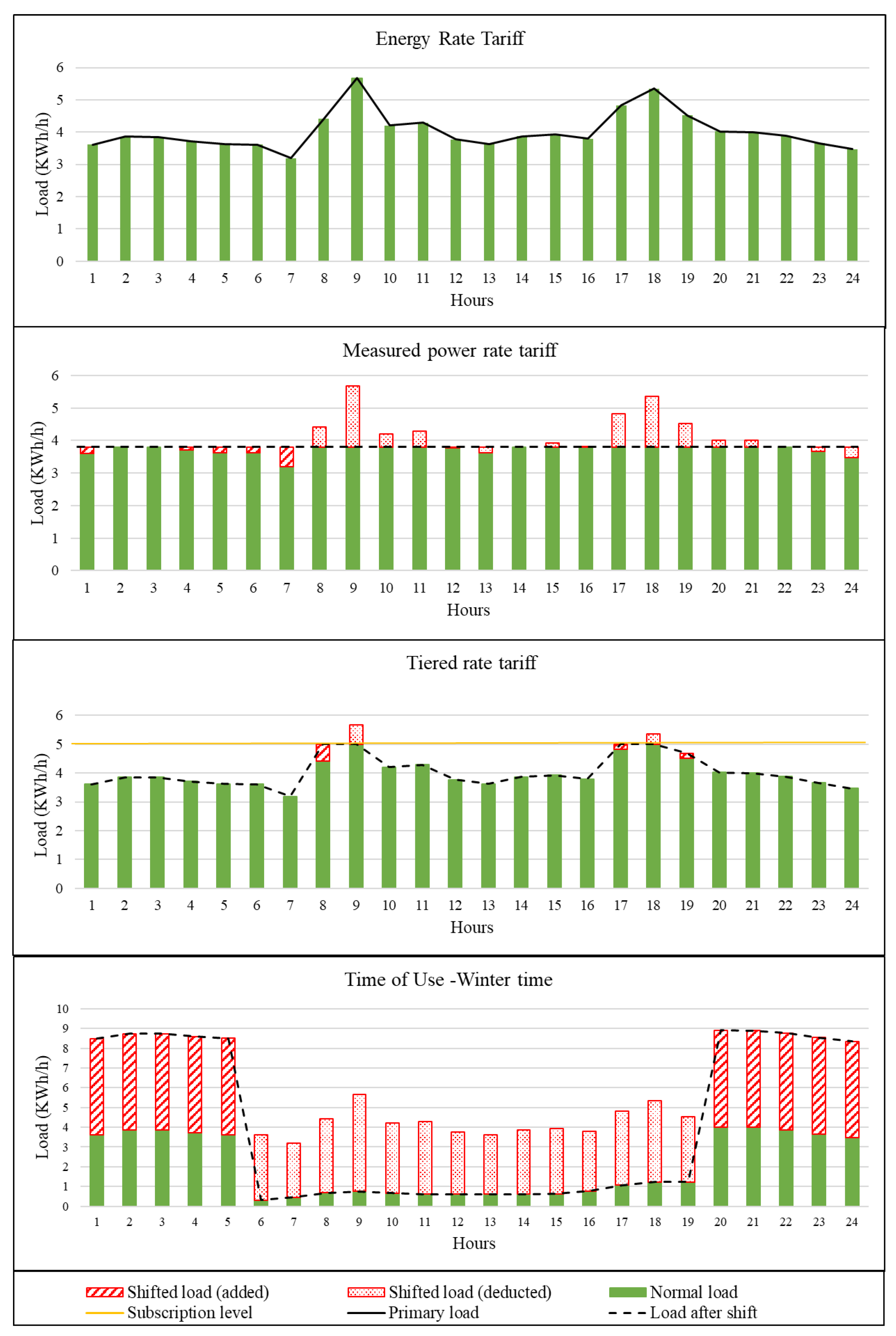
• In the measured power rate tariff, the daily peak power cost is a part of the cost, which can be reduced without having an impact on the demand. The minimum daily peak cost can be achieved when the peak is as low as possible, thus creating a constant load profile after the shift. This constant value is the maximum of the plug load (plug load = total load − heating load) and the daily average heating load. This value is selected to meet the plug load during all hours of the day and minimize the peak of the heating load. If the load profile has smaller peaks distributed across a wide area, the cost reduction will be small. On the other hand, higher peaks of short duration can lead to greater cost reductions. So, the implementation of the ideal load shift is recommended for loads with high peaks with short duration.
• For the tiered rate tariff, the overuse cost can be reduced without impacting the demand. Thus, the heating loads for the hours with demands higher than the subscription level will be shifted to the hours with loads below the subscription level, reducing the overuse cost to zero.
• For the time of use tariff, the heating loads that occur during the penalized hours (winter days, red hours in Figure 2) should be shifted to the normal hours (winter nights, green hours in Figure 2). Because all summer hours have the same energy costs, the ideal heat shift will have no impact during the summer.

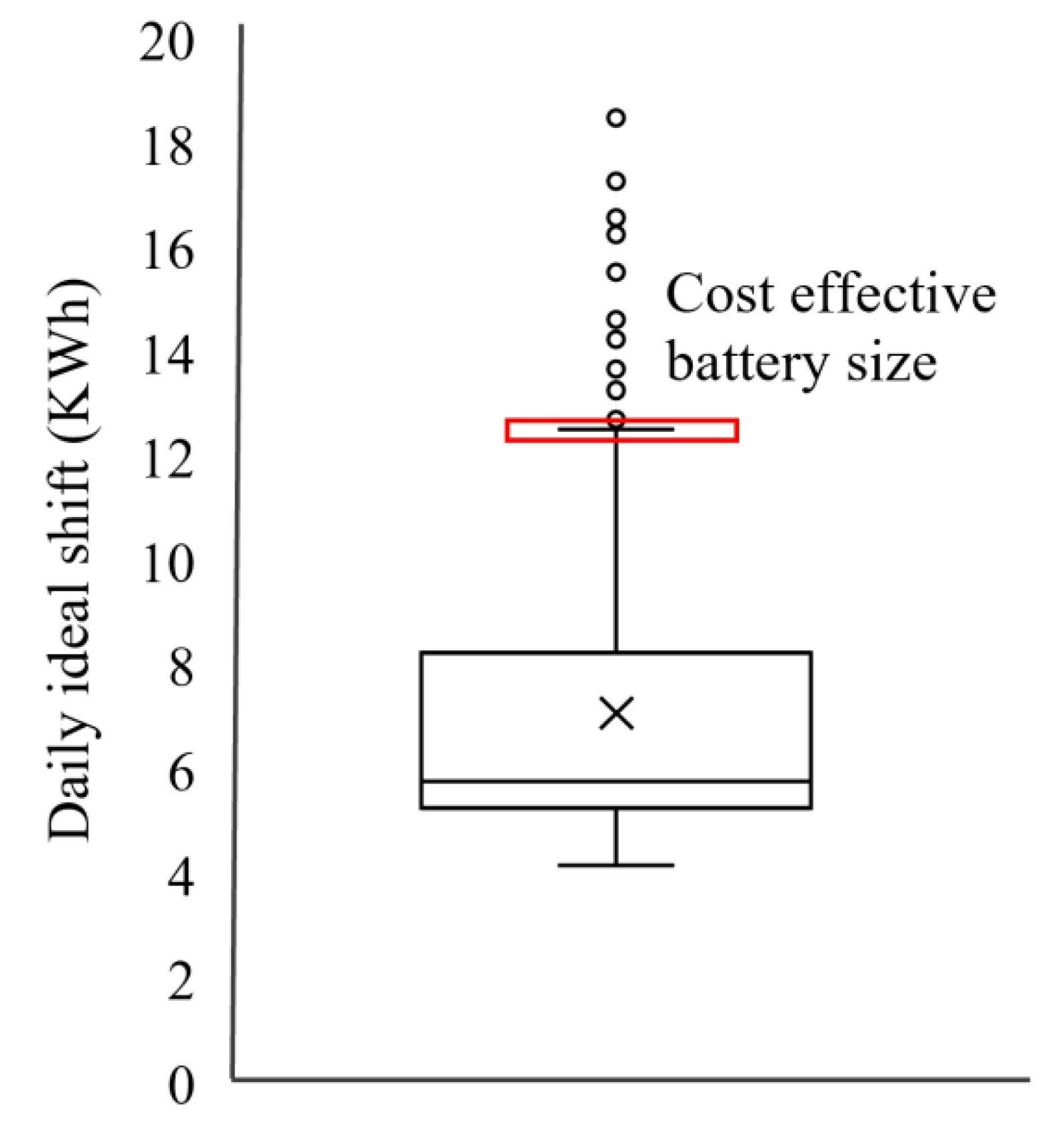
2.2.2. Cost-Effective Battery Sizing and Shift Adjustment

The implementation of battery storage, along with demand side management, is important in terms of increasing self-consumption and reducing peak power periods in the grid [56]. In the Norwegian context, reducing energy use during peak load hours is considered an important objective. For this reason, home storage solutions are gaining importance, and it has been suggested that storage capacities be added to building regulations [57]. Furthermore, the Research Center on Zero Emission Neighborhoods in Smart Cities (FMEZEN) indicates that the introduction of energy storage and smart control methods can be a useful option for reducing energy costs when the new tariffs suggested by the Norwegian regulator are implemented [56]. In addition, even though power outages are rare in high-income countries, batteries can play an important role in buildings’ power supply stability [58]. This study focuses on batteries for storing the daily heat shift and using the stored shift in the batteries as backup storage in case of power outages. Even though, thermal storage (i.e., active or passive) can be considered as possible options for storing daily shift, the focus of this study is on batteries as electrical storage for the shift storage. The strategy used for battery sizing in this paper is called the “cost-effective battery sizing strategy”. This strategy focuses on the daily capacity that is needed for shift storage and selects the cost-effective capacity based on the amount of daily shift storage and its distribution. The cost-effective capacity can cover the storage capacities that have a high probability of happening daily over the course of a year and will be enough for most of the days of the year (not all days of the year). Of course, there will be some days during the year that the cost-effective battery capacity will not be able to cover, but the storage capacities for these days are neglected because they have lower probabilities of occurrence.

The selection of the cost-effective battery size based on the amount of daily storage and its distribution is shown in Figure 5. For example, a design can have a daily storage distribution that is skewed toward the higher levels, leading to a higher battery capacity. Likewise, when the daily storage distribution is skewed toward the lower levels, a smaller battery capacity will be needed. Figure 5 shows the box plot of the daily storage capacity needed for the ideal heat shift in a typical building over the course of a year. The cost-effective battery capacity is based on the maximum capacity necessary in the box plot, which is indicated with a red box ($C_{Bat}$) in Figure 5. It should be noted that this value is not the maximum value in the outlier part. The capacity data in the outlier part of the box plot are neglected in order to concentrate on cost-effectiveness. So, if the distribution of the daily storage has some data in the outlier part of the box plot, then the selected battery capacity may not be sufficient for storing the entire ideal shift (IHS). This lack of storage will deduct some part of the shift from the ideal heat shift, creating what will be called the effective heat shift (EHS) in this paper. It should be noted that when the box plot does not have an outlier section, the EHS will be equal to the IHS. In distributions with outliers, the EHS will be less than the IHS. The deducted part of the shift (the difference between the IHS and EHS) can be stored in large-scale, centralized neighborhood batteries. This paper focuses on just the cost-effective batteries at the building scale and does not consider large-scale, centralized batteries. Furthermore, it should be noted that the cost-effective battery capacity provides a battery size that can be used by designers and decision makers in the concept design stage and it is not capturing the details related to charge and discharge states of the battery, which may be needed in the detailed design stage. This can lead to some energy losses due to the charging and discharging efficiencies and can slightly increase the total energy use of the building, which has been neglected in this study.

2.2.3. Energy Flexibility Quantification

One of the approaches to analyzing energy-flexible buildings is the quantification of the flexibility potential of a building based on its response to a specific signal from energy systems [59,60]. In this approach, flexibility is quantified indirectly by analyzing the changes in the performance indicators, such as energy savings, peak power reductions, cost savings, and reductions in $C{O}_2$ emissions. The quantification method proposed in this study aims at calculating a single indicator (the cost-effective flexibility index (CEFI)), which shows the cost-effectiveness of the implemented battery for storing the heat shift as a flexibility asset. The CEFI divides the percentage of the cost savings achieved by the effective heat shift by the size of the cost-effective battery and creates an index in %/kWh that indicates the percentage savings that can be guaranteed if the cost-effective battery size is implemented in the building. If the implemented battery is smaller than the cost-effective battery size, the percentage of savings will be lower.

2.2.4. Survivability Quantification (Active + Passive)

A large part of the building literature is focused on the passive survivability of a building, which is defined as the ability to maintain the building in a safe thermal condition in the event of an extended loss of grid power [61]. This term is also known as thermal resilience because it focuses on building survivability from the thermal point of view only [62]. Passive survivability considers the length of time that a building remains in habitable thermal condition following a power outage from the grid [63]. The habitable thermal condition encompasses a wider range than the thermal comfort condition. For example, the habitable thermal condition in this paper is considered to be 15 °C $<T_{indoor}<$ 30 °C [63], which is wider than the thermal comfort range for living rooms suggested by the Norwegian standard (19 °C $<T_{indoor}<$26 °C) [64]. The length of time that passes between the onset of a power failure and when the temperature reaches 15 °C is called winter passive survivability. The time that passes between the power failure and when the temperature reaches 30 °C is called summer passive survivability. The sum of these two values constitutes the passive survivability index (PSI) in this work.

$$\mathrm{PSI}=\mathrm{Summer}\mathrm{passive}\mathrm{survivability}+\mathrm{Winter}\mathrm{passive}\mathrm{survivability}$$

(1)

The winter passive survivability and summer passive survivability are calculated by simulating a six-day power failure during the coldest and warmest weeks of the winter and summer, respectively. Because this study is focused on all-electric buildings, a new kind of survivability is introduced in this paper. This survivability is for all-electric buildings equipped with batteries and is called “active survivability”. The term “active” is used here because batteries are added to the buildings as active solutions to protect them from power failures. Furthermore, this survivability focuses on more than the thermal condition, as it evaluates the survivability of all end uses, such as lighting, appliances, and domestic hot water. In this paper, active survivability is defined as the ability of the building and its storage system to maintain critical operations in the absence of grid power and is quantified with the “active survivability index (ASI)”. The ASI divides the cost-effective battery capacity selected for the shift storage by the minimum energy needed for the building to maintain critical operations. Because the suggested survivability in this paper focuses on the survivability of all end uses in an all-electric building, the following assumptions are made when calculating the minimum energy consumption needed to maintain critical operations.

• The building heating setpoint is changed to 15 °C as the habitable threshold.
• The domestic hot water, lighting, and the appliance demand are decreased to 25% of the values suggested by SN/TS 3031 [65].

The simulation of the building designs under these conditions will calculate the minimum energy consumption necessary to maintain critical operations.

2.3. Algorithm Output

Based on the algorithm developed in the previous section, the following variables are defined in order to quantify the flexibility and survivability indexes.

• AC: The annual energy cost of the building without considering a heat shift (€/yr), which can be calculated for each design under the business models of dynamic pricing tariff. This value was calculated in Section 2.2.1.
• ACIS: The annual energy cost of the building using the ideal heat shift (€/yr), which can be calculated for each design under the business models of dynamic pricing tariff. This value was calculated in Section 2.2.1.
• $C_{Bat}$: The cost-effective battery size (kWh), that is needed for storing the shifted heat. This value was determined in Section 2.2.2.
• ACES: The annual energy cost of the building based on the effective heat shift (€/yr), which was calculated in Section 2.2.2.
• $E_{min}$: The minimum energy needed by the building to maintain the critical operation (kWh), which is determined in Section 2.2.4.
• $SI=\frac{\mathsf{\Delta }C}{AC}\times 100$: The savings index (%), which shows the benefit of utilizing a building’s flexibility by dividing the cost savings by the annual costs before the shift, as defined by [9].
• $CEFI=\frac{SI}{C_{Bat}}$: The cost-effective flexibility index (%/kWh), which shows the cost effectiveness of a building’s flexibility by dividing the SI by the cost-effective battery capacity.
• PSI: The length of time that the building can remain in the habitable thermal condition (15 °C $<T_{indoor}<$30 °C) following a power outage from the grid.
• $ASI=\frac{C_{Bat}}{E_{min}}\times 100$: The active survivability index (%), which shows the percentage of the minimum energy needed in the critical condition that can be covered by the cost-effective battery used for shift storage. This value shows how helpful the battery can be in terms of the building’s survival in the absence of power from the grid.

3. Application on the Case Study

A representative model of a Norwegian single-family house [66] was chosen as the case study building based on research conducted by Homaei and Hamdy [67]. This building is a two-story building located in Oslo. It has a floor area of 162 m² and is divided into three zones in a detailed model in the IDA ICE software.The zones consist of a representative dayroom (i.e., a combined zone for living room, kitchen, and entrance), bedroom, and bathroom. Occupancy schedules, domestic hot water distribution, and internal gains are derived from Nord et al. [68]. The developed model has been validated [67] and is flexible in terms of changing the design parameters and adding renewable energy sources (RES). Furthermore, external factors can be altered, such as occupant behavior and weather. This model is shown in Figure 6.

Ten different building designs are suggested for this building model by changing the design parameters, including the building envelop, window-to-wall ratio (WWR), heating system, and implementation of RES. These designs are all competitive designs [67], which means that they all meet the same energy consumption and comfort requirement targets, which have been set based on the TEK 17 standard, the current set of minimum requirements in Norway [64]. For example, one design can achieve the target by combining a low-insulation envelope with very efficient energy and ventilation systems, while another design can achieve the targets via a highly insulated envelope and less efficient ventilation and energy systems. These competitive designs provide the opportunity to compare the flexibility and survivability of various designs having the same energy level. The characteristics of the ten designs are shown in

Table 2. Details of the ten competitive designs considered in the case study demonstration.

	Designs
Design Parameters	D1	D2	D3	D4	D5	D6	D7	D8	D9	D10
Overall U-value (W/m${}^2·$k)	0.31	0.25	0.43	0.36	0.33	0.29	0.51	0.44	0.40	0.35
Normalized thermal bridge (W/m${}^2·$k)	0.05	0.03	0.07	0.05	0.03	0.02	0.06	0.07	0.06	0.05
WWR (%)	30	30	30	30	40	40	40	40	30	30
Heating system	ER	ER	ASHP + ER	ASHP + ER	ER	ER	ASHP + ER	ASHP + ER	ER	ER
Ventilation system	Balanced	Exhausted	Balanced	Exhausted	Balanced	Exhausted	Balanced	Exhausted	Balanced	Balanced
Solar DHW system size (m${}^2$)	0	5	0	0	0	5	0	0	0	0
PV system size (m${}^2$)	0	0	0	0	0	0	0	0	40	20
Lighting	Typical	LED	Typical	Typical	Typical	LED	Typical	Typical	Typical	Typical
KPI
Total energy consumption (kWh/m${}^2$)	110	110	110	110	110	110	110	110	110	110

. From the envelope point of view, the overall U-value, the normalized thermal bridge, and the WWR ratio have been changed. The design options for heating system include direct electric heating with electric radiators with efficiencies near 99%, and the combination of electric radiators and indirect electric heating with an air source heat pump with a coefficient of performance (COP) of 3.2. Hence, the COP of the heat pump can decrease due to the low outside temperature during winter; as such, it has been combined with electric radiators in order to prevent undercooling. Options for the ventilation system include balanced mechanical ventilation with a heat recovery unit that has an efficiency of 80% and mechanical exhaust ventilation without a heat recovery unit. For lighting, in most of the designs, typical lighting (luminous efficacy of 12 W/m) is implemented, but in the designs with high energy demand, LED lighting (luminous efficacy of 60 W/m) is used in order to keep the total energy demand lower. In some designs, renewable energy systems such as solar thermal collectors (STC) or photovoltaics (PV) are implemented. Heat loss is neglected in all of the designs. It can be seen from Table 2 that all of these designs meet the energy consumption target for the building, which is 110 kWh/m² based on the TEK17 standard. Furthermore, buildings face various uncertainties during their operation and their performance can deviate from the set target. There are studies that evaluate the impacts of uncertainties on building performance. These uncertainties can be categorized as, for example, climate change [69], changes in economic factors [70], and variation in occupant behavior [71]. Other studies evaluate the impacts of uncertainties on the energy flexibility of buildings. For instance, Hu et al. [72] quantified the uncertainties related to occupancy and occupant behavior in terms of the aggregated energy flexibility in high-rise residential building clusters. Arteconi et al. [12] evaluated the influences of weather data and stratigraphy on the flexibility performances of buildings with electric heating and cooling systems. Hence, 16 different occupant behavior and weather scenarios are considered in this study. For the climate uncertainty, two climate files from The American Society of Heating, Refrigerating, and Air Conditioning Engineers (ASHRAE), IWEC and IWEC2, are used from the library of IDAICE [52]. For occupant behavior uncertainties, two heating setpoints, two shading strategies, and two window opening strategies were modeled. Further details regarding the modeling assumptions for occupant behavior and weather can be found in Homaei and Hmady’s study [67] and Appendix A. The performance of each design was simulated across the 16 scenarios in IDA ICE. The total load profiles were then extracted from IDA ICE and imported into the algorithm developed in Section 2.2 to calculate the energy cost, the cost-effective battery size, and the CEFI, PSI, and ASI under the three dynamic pricing tariffs.

4. Results and Discussion

As mentioned previously, in order to test the algorithm and evaluate the impacts of the occupant and weather uncertainties on a building’s energy flexibility and survivability under different tariffs, the procedure explained in Section 2 was applied to the building models described in Section 3. The results are described in the following subsections. It should be noted that the results in each subsection are analyzed according to the designs and tariffs.

4.1. Cost and Shift Analysis

The energy demands of the ten designs have been investigated under 16 occupant and weather scenarios. The algorithm developed in MATLAB uses the hourly energy demand for each building design to compute its annual energy costs and the ideal and effective heat shifts for the four tariffs. Figure 7 shows the resulting annual costs (before and after the shifts) and effective load shifts. The following results can be obtained from Figure 7.

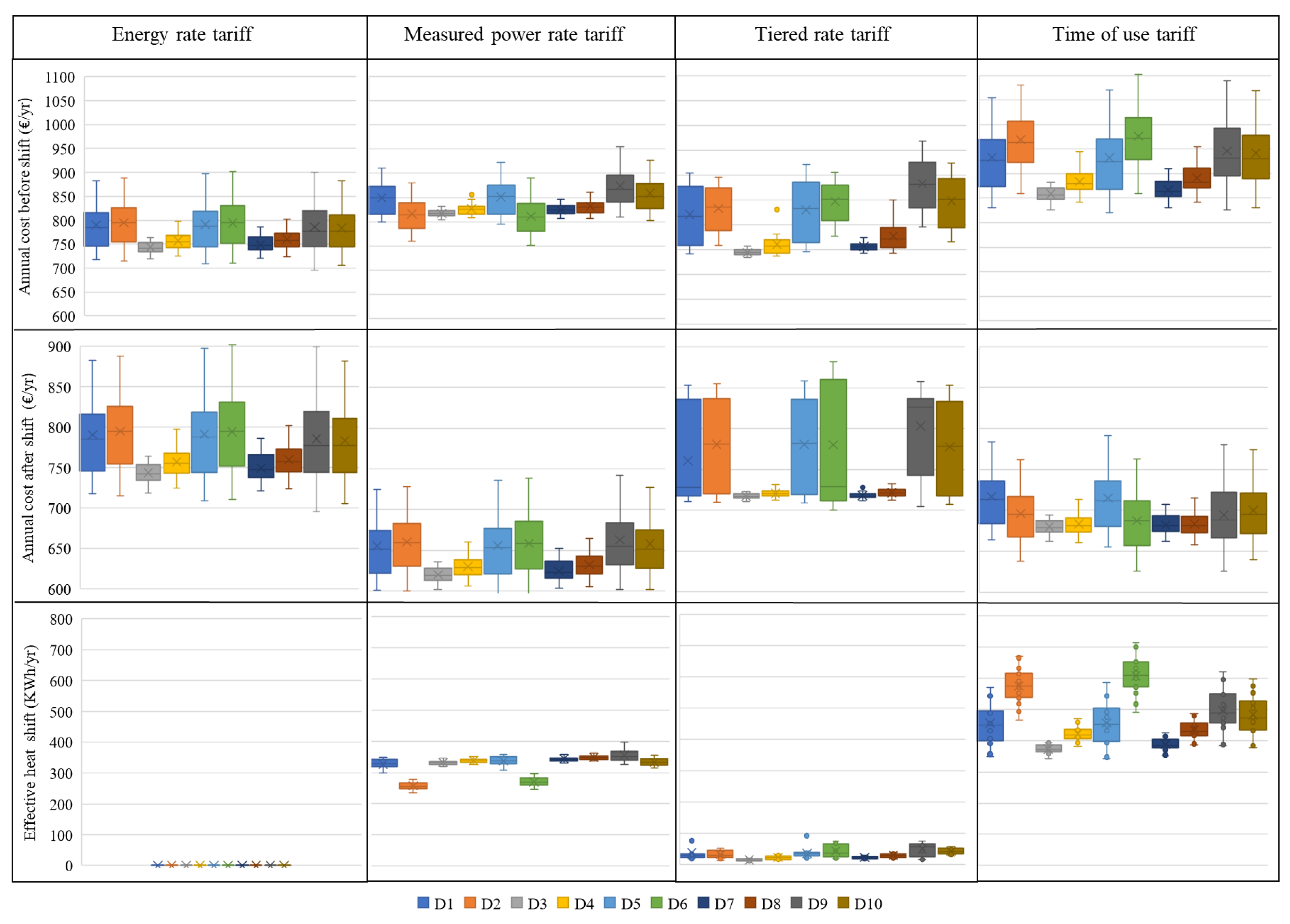
4.1.1. Annual Energy Costs before and after the Shift

First, the tariffs are compared in terms of costs, then a cost comparison is done for the different designs. In the base condition (without a shift), the cheapest tariff is the energy rate tariff across all design. This result makes sense because the energy rate tariff does not apply penalties and simply reflects the price of energy consumption. Furthermore, for most of the designs in the base condition, the most expensive tariff is the time of use tariff. A comparison of the tariffs without a shift shows that if customers do not change their load profiles under the tariffs, they will face an increase in grid rent. In other words, these tariffs should be viewed as incentives for the customers to change their consumption patterns. If the effective shift is applied, the energy rate tariff is the most expensive tariff because it has no shift. The measured rate tariff has the minimum annual cost after the effective shift for most of the designs. The comparison of the annual costs before and after the shift reveals that the time of use tariff leads to the higher cost savings among the three tariffs with a shift. So, this tariff provides higher incentives for changing consumption patterns; however, it has a higher annual cost than the rest before the shift.

For the design comparison, the simulation results show that designs equipped with the combination of an electric radiator, ASHP, and balanced ventilation are less sensitive to uncertainties in comparison to the designs incorporating an electric radiator and exhaust ventilation. For example, in a scenario designed to increase the energy consumption, the increases in the amount of energy and the peak value needed for designs featuring an electric radiator will be greater than those for designs with an ASHP. The same holds true for balanced and exhaust ventilation. For this reason, Figure 7 shows that the average annual energy costs for the designs incorporating an ASHP ($D_3$, $D_4$, $D_7$, $D_8$) are less than the annual costs for the designs featuring just an electric radiator or exhaust ventilation ($D_1$, $D_2$, $D_5$, $D_6$, $D_9$, $D_{10}$) for the energy rate tariff, the time of use tariff, and the tiered rate tariff. Furthermore, for designs with the same energy system (e.g., $D_3$, $D_4$, $D_7$, $D_8$) and designs with air-balanced ventilation (e.g., $D_3$, $D_7$) have lower annual costs than the designs with exhaust ventilation (e.g., $D_4$, $D_8$). Under the measured power rate tariff, the situation is a bit different. For this tariff, the annual costs before the shift for designs $D_2$ and $D_6$ are less than the costs for other designs featuring an electric radiator. These two designs incorporate LED lights, and they have a smaller plug load compared to the other designs, decreasing their peak power costs during the summer compared to the other designs. In the other words, the main difference between $D_2$ and $D_6$ and the rest of the designs is that they require less peak power during the summer. A comparison of the daily shifts across a year for $D_2$, $D_6$, and $D_1$ (a typical design without LED lights) is shown in Figure 8. This figure shows that there are significant differences among the daily shifts for designs $D_2$, $D_6$, and $D_1$ during the summer. The LED lights, used to compensate for the higher demand (created by the implementation of the exhaust ventilation and electric radiator), are responsible for the observed differences.

If the effective shift is applied, the annual costs for the designs with a combination of an ASHP and electric radiator ($D_3$, $D_4$, $D_7$, $D_8$) are lower than the annual costs for the designs featuring an electric radiator only ($D_1$, $D_2$, $D_5$, $D_6$, $D_9$, $D_{10}$), except in the case of the energy rate tariff, for which no shift occurs. Furthermore, designs with higher costs in the base condition (without the shift) achieve greater cost reductions when the load shift is applied (e.g., designs featuring an electric radiator and exhaust ventilation).

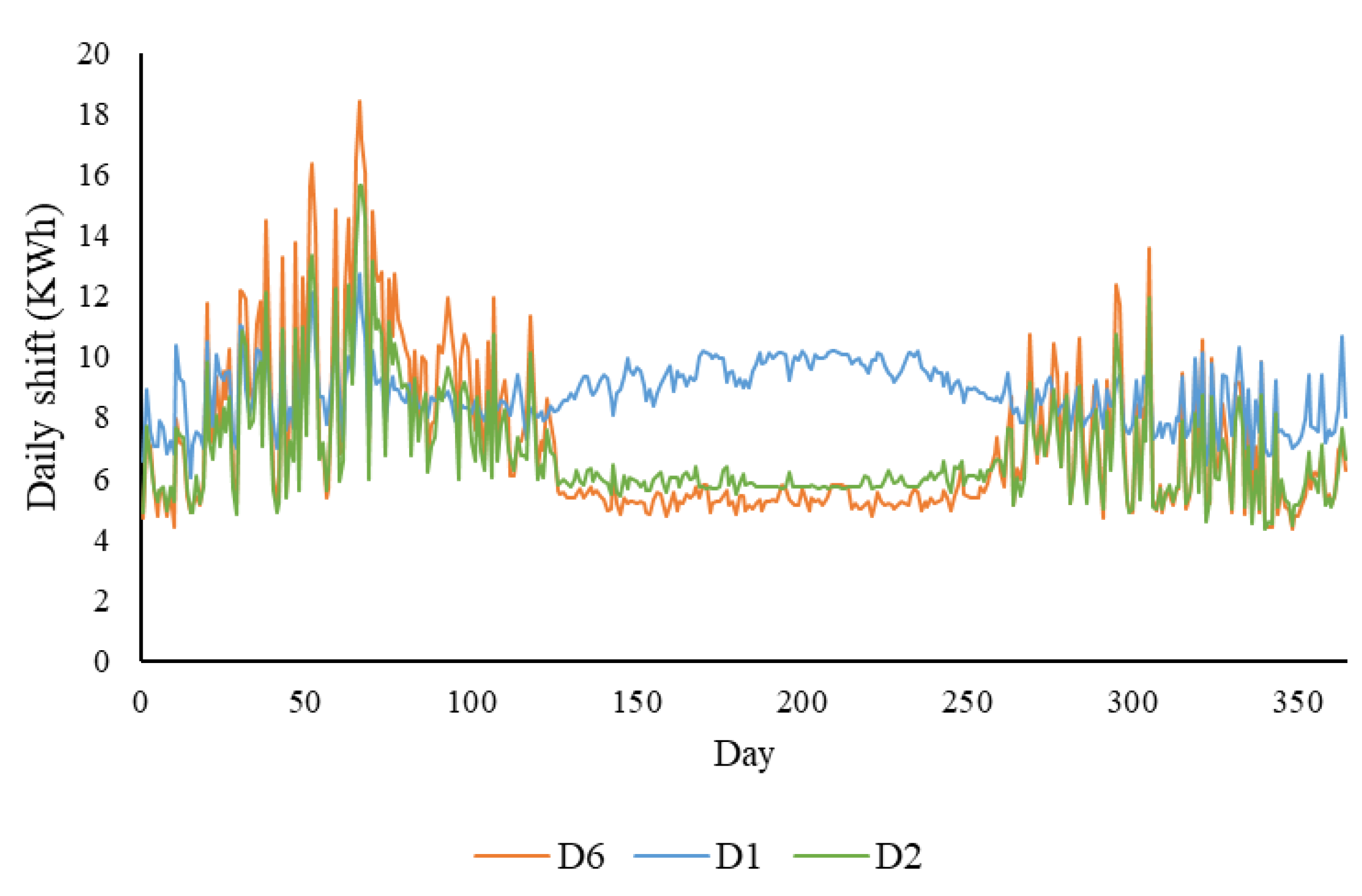
4.1.2. Effective Heat Shift

A comparison of the effective shifts for the three business models of dynamic pricing tariff shows that based on cost-effective battery sizing, the effective shifts for the time of use tariff and the tiered rate tariff are the highest and lowest, respectively. The effective shift for the measured power rate falls between the shifts for these two tariffs. The time of use tariff shifts the total daily heating demands to the night periods. The case study building is a heat-dominated building, and the daily heating demand is a large part of its total energy consumption. Hence, the time of use tariff has the greatest effective heat shift. For the measured power rate tariff, all demand higher than the constant value (flat load profile) is shifted. Because the constant value is calculated based on a comparison of the daily heat average and plug loads, there is a surplus for all days of the year, but this surplus can vary from very low to high amounts. Hence, the shift is distributed across the year and creates a medium daily shift in comparison to the two other tariffs. Because the shift is distributed across the year, under the measured power rate tariff, the battery will go through more charge and discharge cycles, which can have negative effects on the battery life. For the tiered rate tariff, any demand exceeding the subscription level is shifted. Because the subscription level is not related to the daily distribution of load, the shift hours are random and skewed toward the winter peak consumption hours. This focus on the peak hours results in a lower daily shift for this tariff.

When it comes to the effective heat shift comparison between designs, it can be seen that for the measured power rate tariff, $D_2$ and $D_6$ have the smallest shifts. The shift for the measured power rate tariff is based on values that are higher than the constant value across the year. Thus, $D_2$ and $D_6$, which have lower plug loads, have smaller shifts during the summer compared to the other designs (Figure 8). Thus, they have the smallest shifts among all designs. Regarding the time of use tariff, because the daily heat consumption is shifted, designs featuring greater daily heat consumption have bigger shifts. These designs include those with weaker envelopes and electric radiators ($D_9$, $D_{10}$) or the ones with exhaust ventilation in combination with an electric radiator ($D_2$, $D_6$). As for the rest of the designs, the ones featuring just an electric radiator ($D_1$, $D_5$) have higher daily heating demands and consequently higher shifts than the ones using an ASHP and electric radiator ($D_3$, $D_4$, $D_7$, $D_8$). For the tiered rate tariff, the shift is focused more heavily on the peak hours during the heating period; hence, designs with more heating peaks will have greater shifts. These designs include those with weaker envelopes and combinations of electric radiators and exhaust ventilation systems. The smallest shifts under this tariff are seen for designs equipped with ASHP and an electric radiator. Designs with balanced ventilation have smaller shifts compared to the designs incorporating exhaust ventilation due to their lower peaks.

4.2. Cost-Effective Battery Size

The other important parameter, which was introduced in Section 2.3, is the cost-effective battery capacity for the shift storage. Figure 9 shows the relationship between the SI and cost-effective battery capacity as well as a detailed comparison of the cost-effective battery capacities for the ten designs across all tariff and reference scenario combinations. It can be seen that the SI and cost-effective battery capacity are directly proportional for all of the tariffs. Figure 9 reveals that the time of use tariff has the highest SI and cost-effective battery capacity due to the large shift for this tariff, which was discussed in Section 4.1.2. It should be noted that, in addition to the amount of the shift, the daily shift distribution also plays a role in determining the cost-effective battery capacity, as is discussed later. Under the time of use tariff, homeowners can achieve higher cost savings, but they will need greater storage capacity to do so. In contrast, the tiered rate tariff needs very low storage capacity, but it leads to lower cost savings due to its smaller shift. The measured power rate tariff falls between the other two tariffs in this regard. It has an SI in the range of the SI for the time of use tariff but a significantly lower cost-effective battery capacity featuring many charge and discharge cycles.

The battery capacity is determined according to the daily shift and its distribution. Hence, violin plots have been used to plot the distributions and probability densities of the daily shifts for the ten designs. The violin plot is similar to the box plot and provides a kernel density estimation of the underlying distribution. These violin plots, along with the relationships between SI values and cost-effective battery capacities for the tariffs in the reference scenario, are shown in Figure 9. Note that the cost-effective batteries are only used for the storage of the shifted heat and not for storing energy produced by renewable energy sources. Based on this figure, the measured power rate tariff produces more distributed daily storage in $D_2$, $D_6$, $D_9$, and $D_{10}$, and the standard deviations in the daily storage are higher for these designs in comparison to the other designs. In contrast, designs $D_3$, $D_4$, $D_7$, $D_8$ have less daily storage, and their distributions are dense in the middle. Thus, the most important parameter in the classification of the designs regarding the cost-effective battery capacity pertains to the energy system. Designs $D_9$ and $D_{10}$ have a weaker envelope in combination with an electric radiator, resulting in higher daily shifts and increased battery capacity. Even though $D_2$ and $D_6$ have lower shifts due to lower summer usage, their shifts are higher during the winter due to the exhaust ventilation and electric radiator, leading to increased battery capacity. The remaining designs $D_1$ and $D_5$ have data distributed at the higher level in comparison to designs $D_3$, $D_4$, $D_7$, and $D_8$, leading to higher cost-effective battery capacities. The smallest battery capacities are assigned to the designs with the combination of an ASHP and electric radiator because their daily storage values are concentrated at the lower levels (the heating demand created by a heat pump has less variation than the heat demand created by an electric radiator, leading to smaller surpluses for the shift). For the designs without an ASHP, air-balanced ventilation leads to smaller cost-effective battery capacities due to fewer deviations in the heating demand across a year. The shift in the time of use tariff is focused on daily heat consumption. So, designs with higher daily heat consumption will have higher battery capacities. Figure 9 shows that designs with higher heating demands also have shifts that are distributed more widely. These designs include those with weaker envelopes and electric radiators ($D_9$, $D_{10}$) or exhaust ventilation and an electric radiator ($D_2$, $D_6$). Designs $D_1$, $D_5$ have greater shifts and more widely scattered daily storage requirements, resulting in mid-level cost-effective battery capacities and SI values. The smallest cost-effective battery capacities and SI values belong to the designs featuring ASHPs and electric radiators due to their smaller shifts and dense distributions. Design $D_3$, which uses a combination of an ASHP, electric boilers and balanced ventilation, has the minimum cost-effective battery capacity.

For the tiered rate tariff, the shifts occur during random hours and more frequently during the peak hours in the winter. For this reason, designs with higher demand during the winter will have greater shifts and higher SI values, as seen in the designs $D_2$, $D_6$, $D_9$, and $D_{10}$, which have weaker envelopes with an electric radiator or exhaust ventilation with an electric radiator. On the other hand, these designs have more widely distributed daily storage and cost-effective battery sizes. Other designs with an electric radiator or an ASHP and an electric radiator have SI values and cost-effective battery sizes that are smaller than those for the previous group. For this tariff, the minimum battery capacity is also assigned to design $D_3$, with the electric radiator, ASHP, and balanced ventilation.

4.3. Cost-Effective Flexibility Index (CEFI)

The cost-effective flexibility index (CEFI) is introduced in Section 2.3. This parameter indicates the percentage of savings that can be guaranteed if the cost-effective battery capacity is implemented. Figure 10 compares the CEFIs for the ten designs across the three business models of dynamic pricing tariff under the reference scenario. Comparing the tariffs reveals that in the reference scenario, the percentage of savings per kWh achieved by the cost-effective battery capacity across all of the designs is higher for the measured power rate tariff. For this tariff, the cost savings are greater than those for the tiered rate tariff, and the battery capacity is as great as that for the time of use tariff, leading to the highest CEFI. The tariff with the next-highest CEFI is the tiered rate tariff, while the time of use tariff has the minimum CEFI due to its very high battery capacity. Therefore, the measured power rate tariff saves more money at a smaller battery capacity.

When it comes to the design comparison across all of the tariffs, the highest CEFI is related to $D_3$. The other designs with high CEFIs are $D_7$, $D_4$, and $D_8$, all of which have an ASHP and electric radiator. Among these four designs, $D_3$ and $D_7$, which have air-balanced ventilation, have higher CEFIs compared to designs $D_4$, $D_8$. Of the remaining designs, those with weaker envelopes and electric radiators ($D_9$, $D_{10}$) or exhaust ventilation and electric radiators ($D_2$, $D_6$) have the smallest CEFIs. Based on the suggested design options in this paper, it can be concluded that the most highly recommended design options for increasing the CEFI are those with ASHP and balanced ventilation. PVs must be paired with weaker building envelopes to meet the same energy target and for this reason, designs with PVs have larger battery size and smaller CEFI.

4.4. Survivability

The results related to the survivability can put into two categories: passive survivability and active survivability.

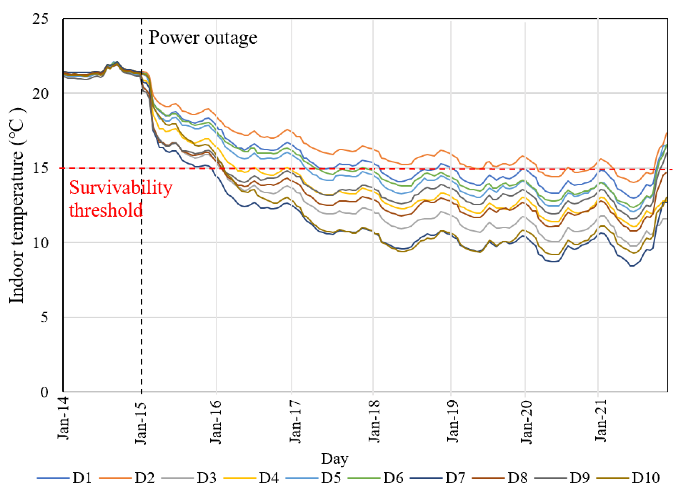
4.4.1. Passive Survivability

The case study building is a heat-dominated building and no cooling systems have been considered. In order to analyze passive survivability, a week is selected in each of winter and summer to run simulated grid power failures. The simulations are run by shutting off the power (for the HVAC and other energy-consuming equipment, such as appliances) during the warmest and coldest periods in summer and winter, which are selected from a typical year data in the IDA ICE weather file. For the summer passive survivability, a six-day power failure is applied starting on 15 July (the warmest week in the weather file). Because the building is a heat-dominated building, there is no need for cooling systems; hence, applying the power failure in the summer does not increase the temperature in the house to beyond the range of habitable conditions ($T_{Indoor}>$ 30 °C) in any of the designs. This means that all of the designs retain the habitable thermal condition in the case of a grid power failure in the summer. Thus, the PSI will reflect only the winter passive survivability for the current case study. For the winter passive survivability, a six-day grid power failure is applied starting on 15 Jan (the coldest week in the weather file). During this period, all of the designs experience temperatures below the habitable temperature ($T_{Indoor}<$ 15 °C). Figure 11 shows the winter passive survivability performances for the ten designs for a power failure starting on 15 January, Ozkan et al. indicate that the building envelope and WWR are the most effective parameters for increasing passive survivability [62]. The results achieved in this paper confirm this fact, and $D_2$, with the strongest building envelope and smaller WWR, has the best passive survivability performance. $D_6$ also has higher passive survivability due to having the second strongest envelope. $D_1$ and $D_5$ have mid-level survivability. The remaining designs, which have ASHPs, have lower survivability performances because the ASHP requires a weaker building envelope to meet the energy target. The designs with PV are in the same situation because they have weaker envelopes.

4.4.2. Active Survivability

The ASI measures how much the cost-effective battery can contribute to the building’s survival in the absence of grid power. The higher the ASI, the higher the self-sufficiency of the building during a power outage. This means that the building can survive with its own storage system, without being dependent on the centralized storage in the larger scales such as neighborhoods. To calculate ASI, the minimum energy that is needed for survivability is estimated by running a simulation for each design in the critical condition. The ASI is calculated by dividing the cost-effective battery size by the minimum energy need for the design. The designs are then compared with respect to maintaining not only habitable temperatures but also meeting the minimum energy needed for other end uses, such as appliances, lighting, and domestic hot water. Figure 12 shows the ASIs for the ten designs for the reference scenarios and the three business models of the dynamic pricing tariffs.

It can be seen that the ASI for the time of use tariff is higher than that for the measured power rate tariff, which in turn is higher than that of the tiered rate tariff because, although the minimum energy needed for survivability is the same for all of the tariffs, the cost-effective battery size is the highest for the time of use tariff. In the higher cost-effective battery range, the building can survive longer on the stored shift in the battery when the grid power fails. Thus, when the time of use tariff is used, the building will be less dependent on large-scale, centralized storage. In contrast, if the tiered rate tariff is implemented, the building will be more dependent on centralized storage during a grid power failure. The ASI comparisons for the designs under each tariff are also informative. It should be noted that the minimum energy needed for survivability changes across the designs; however, the designs are competitive and have the same energy target, so the minimum energy needed for survivability does not vary much across designs. Thus, the cost-effective battery size has more influence on the ASIs of designs with the same energy target. For example, the measured power rate tariff designs $D_2$, $D_6$, $D_9$, and $D_{10}$ have higher battery capacities in comparison to designs $D_1$ and $D_5$ and the designs with an ASHP, namely $D_3$, $D_4$, $D_7$, and $D_8$. The same trend can also be observed for the ASI. The same trend occurs for the tiered rate and the time of use tariffs, and designs with weaker envelopes and electric radiators ($D_9$, $D_{10}$) or exhaust ventilation and electric radiators ($D_2$, $D_6$), which have higher shifts and battery capacities, have higher ASIs in comparison to the designs with ASHPs ($D_3$, $D_3$, $D_7$, $D_8$) or medium envelopes with balanced ventilation ($D_1$, $D_5$). The bigger the cost-effective battery capacity, the longer the building will survive and the less dependent it will be on centralized storage when the grid power fails.

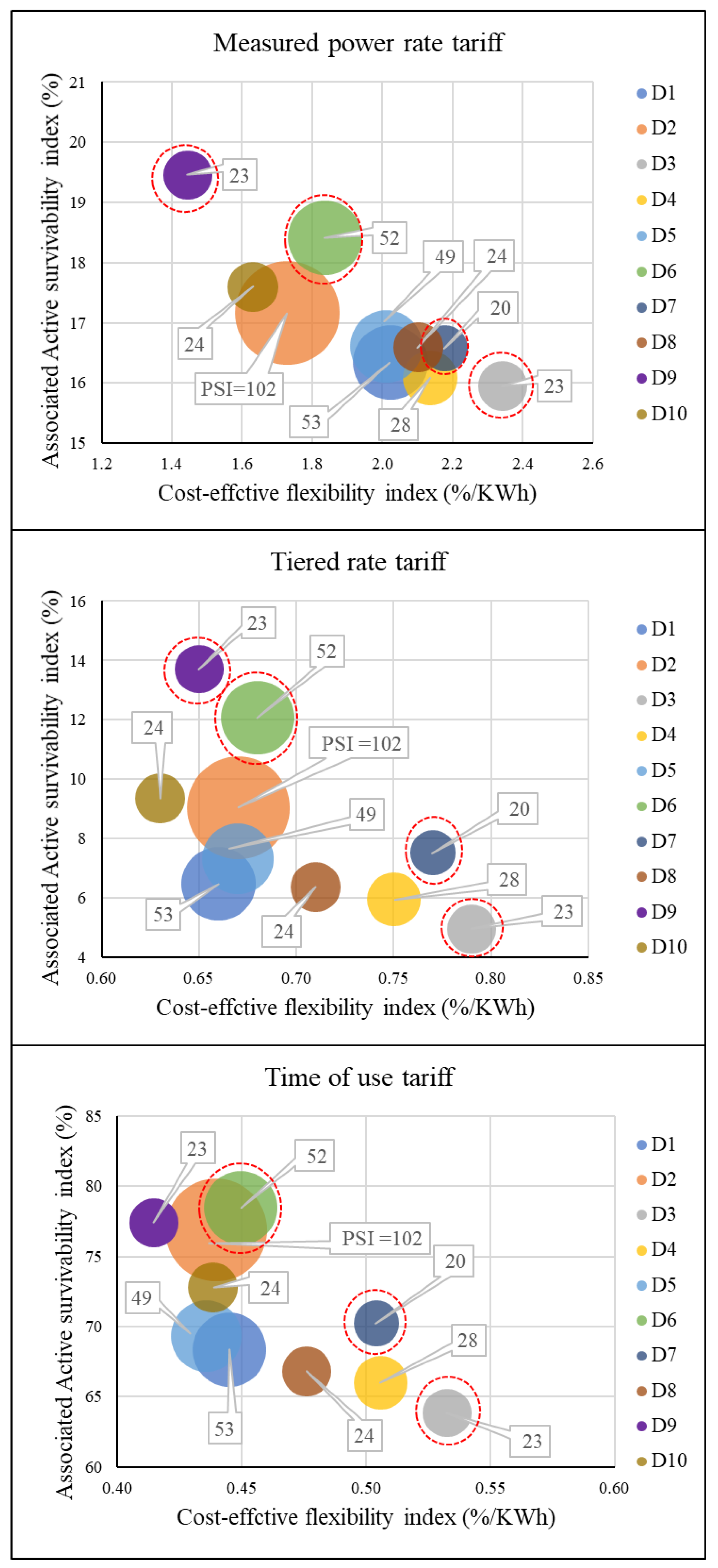
4.5. The Trade-Off between Energy Flexibility and Survivability

The trade-offs between cost-effective energy flexibility and survivability for the ten designs are shown in Figure 13 for the three business models of dynamic pricing tariff. In this figure, the ASI and the CEFI are shown along the x- and y-axes, respectively. The bubbles are added as a third dimension and indicate the relative values of the passive survivability indexes (number of hours that the building can survive). The larger the bubble size, the more passively survivable the building. This figure can help decision-makers to select the best design based on their preferences in terms of cost-effective flexibility, active survivability, and passive survivability. For example, for hospitals and care homes, where the risk associated with a grid power failure is high, the building survivability can be prioritized. In contrast, if the building should ensure a well-functioning DR program, energy flexibility becomes more important and can be prioritized. For example, under the measured power rate tariff, if the decision-maker prefers to achieve savings of more than 2% by utilizing each kWh stored in the cost-effective battery, the passive survivability will be in the range of one day, and the active survivability will be low (less than 17%). This situation comes up in designs with ASHPs and can yield appropriate solutions if the CEFI is prioritized. Another example involves desiring a high ASI value under the time of use tariff. If the decision-maker wants a high ASI value (more than 75%), the CEFI will be low, but the passive survivability can be extended to four days. This situation applies to designs $D_2$, $D_6$, $D_9$, and $D_{10}$. Among these designs, designs $D_2$ and $D_9$ have the greatest passive and active survivability, respectively. When considering all of the tariffs, it can be seen that designs with ASHP have the highest CEFIs and designs with PVs or STCs have the highest ASIs. The competitive designs from the flexibility and survivability points of view are marked with red dotted circles in Figure 13. The competitive designs under the measured power rate tariff are $D_3$ and $D_7$, both of which use ASHP and balanced ventilation and thus have higher CEFIs, as well as $D_6$, which has exhaust ventilation in combination with a strong envelope and STC, and $D_9$, which has a weaker envelope and an electric radiator and thus demands a higher battery capacity (which leads to higher active survivability). Three of these designs have passive survivability values of around one day, and only $D_6$ has higher passive survivability. Hence, if the CEFI is prioritized under this tariff, $D_3$ and $D_7$ can be appropriate solutions, while, if survivability is more important, $D_2$ or $D_9$ could be selected. Under the tiered rate tariff, the competitive designs remain the same due to their similar strategies for the heat shift. Under the time of use tariff, the situation is a bit different, and the competitive solutions are designs $D_3$, $D_7$, and $D_6$. Design $D_9$ is not in the group of competitive designs because the shift strategy for this tariff does not focus on peak demands and limits but rather the total amount of daily heat and shifting the load to the night. When the CEFI is prioritized, designs $D_3$ and $D_7$ are the suggested solutions, while, if survivability is more important, $D_6$ can be an appropriate solution. In general, the methodology in this paper provides information that allows decision-makers, such as grid companies, building designers, and home owners, to set up trade-offs between energy flexibility and survivability from a cost-effective perspective. The decision-makers should select their preferred design based on prioritizations of the involved criteria.

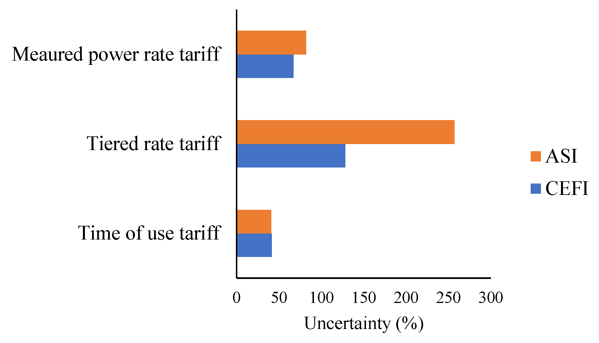
4.6. Impacts of Weather and Occupant Uncertainties

As stated previously, 16 uncertainty scenarios consisting of pairings of two climate scenarios with eight occupant scenarios are considered in this study in order to evaluate their impacts on the indexes under different tariffs. For example, Appendix A shows how annual energy consumption, SI, and cost-effective battery capacity change across the 16 scenarios for the measured power rate tariff. Based on this figure, there is an increase in the SI value and battery capacity, when the total energy consumption increases. In order to discover how these scenarios influence the cost-effective energy flexibility and the active survivability in the three business models for the dynamic pricing tariff, the CEFIs and ASIs are calculated for all designs across all scenarios. The uncertainties in the CEFIs and ASIs across the three business models are calculated and shown in Figure 14. The uncertainty in the CEFI is defined as follows [73]:

$$Uncertainty=\frac{CEF{I}_{max}-CEF{I}_{min}}{CEF{I}_{mean}}\%$$

(2)

where $CEF{I}_{mean}$ is the mean value of the CEFI of all designs across all scenarios and $CEF{I}_{max}$ and $CEF{I}_{min}$ are the maximum and minimum CEFI values for all designs and all scenarios. The same formulation is also used for the calculation of the uncertainty in the ASI. The maximum uncertainties for the CEFI and ASI occur under the tiered rate tariff because the annual subscription level’s direct influence on the SI value, the cost-effective battery capacity, and thus the CEFI and ASI values make this tariff more sensitive to uncertainties in comparison to the other tariffs. In other words, under the tiered rate tariff, when the shift analysis is done, the values related to the CEFI and ASI will be very sensitive to future uncertainties. Hence, it is important to consider uncertainty scenarios when determining a subscription level. The measured power rate tariff has the smallest uncertainties for the ASI and CEFI. Furthermore, as mentioned earlier in Section 2.2.2, the cost-effective battery size covers the storage capacities that have a high probability of happening daily over a course of a year (the loads lower than the red box in Figure 5). With this strategy, there will be some days with low probable loads that the cost-effective battery capacity will not be able to cover them. Given this, uncertainties such as climate change can have some impacts on the battery size and in consequence on ASI and CEFI. If climate change leads to some low probable extreme condition, the cost-effective battery capacity will not get influenced and this is because the cost-effective battery size is independent of extreme conditions. However, if climate change leads to more probable extreme conditions and it completely changes the distribution of the daily loads, the cost-effective battery will not be reliable anymore for the new climate conditions. So, it is recommended to consider the impact of uncertainties on the battery size in the design step.

5. Summary and Conclusions

This paper explores the trade-off between energy flexibility and survivability of all-electric buildings by suggesting a methodology for quantifying the energy flexibility and survivability. This quantification is done with a focus on sizing cost-effective batteries, which can be considered as flexibility assets when they store the shifted heat (as a DR strategy) in the response to a dynamic pricing tariff. In addition, these batteries can be used as backup storage systems for building survival during grid power failures. The energy flexibility is quantified as a single indicator (cost-effective flexibility index) reflecting the amount of cost savings that can be achieved by implementing the cost-effective battery. The active survivability of the building is also quantified as a single indicator (active survivability index) showing how well the cost-effective battery implemented for shift storage can cover the minimum energy needed in the case of a grid power failure. A MATLAB-based algorithm, coupled with dynamic building performance simulation software (i.e., IDA ICE), is used to determine the cost-effective battery size, CEFI, and ASI. This generic method can be used for buildings in cold or hot climates that use electricity as their source for heating and cooling demands. The suggested methodology can be used by different stakeholders in building projects, such as grid companies, building designers, and electric grid customers, including home owners, to estimate the energy flexibility and survivability of the building from a cost-effective perspective. In order to create the conditions necessary for comparing the energy flexibility and survivability of building designs with the same energy target, a unique design space with ten competitive designs is created for an all-electric Norwegian single-family house. Furthermore, 16 uncertainty scenarios are created to evaluate the impact of possible uncertainties on the introduced indexes under different dynamic pricing tariffs. The implementation of the suggested methodology in this case study has created the opportunity to compare three business models for the dynamic pricing tariff suggested by the Norwegian regulator and also to compare designs meeting the same energy target. The following conclusions can be drawn based on this study:

• For all of the suggested designs with the same energy target, the energy rate tariff and the time of use tariff are the cheapest and the most expensive tariffs, respectively. The high prices of the three suggested tariffs are exactly in line with the logic behind them, which is creating incentives and encouraging customers to change their energy consumption patterns.
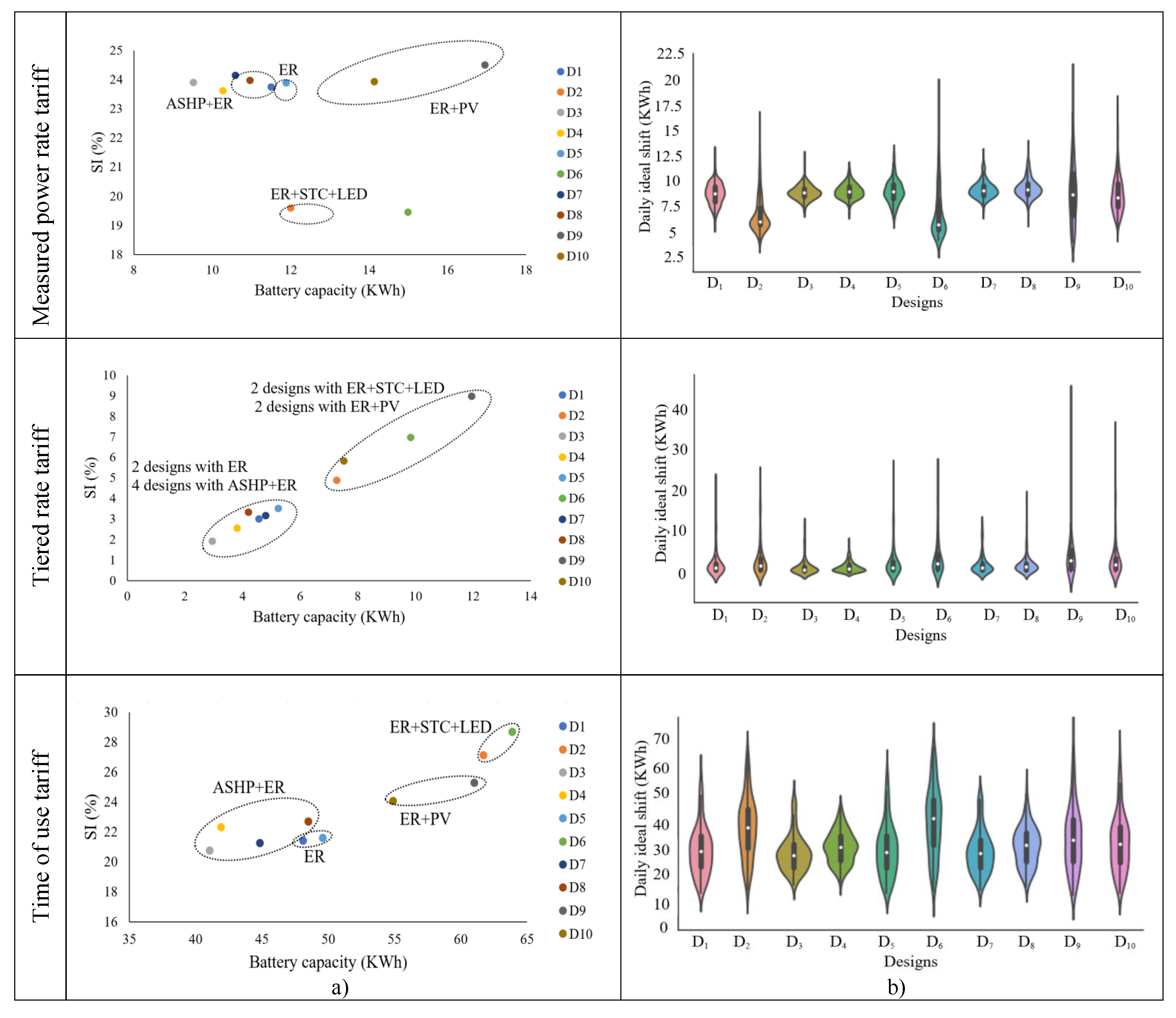
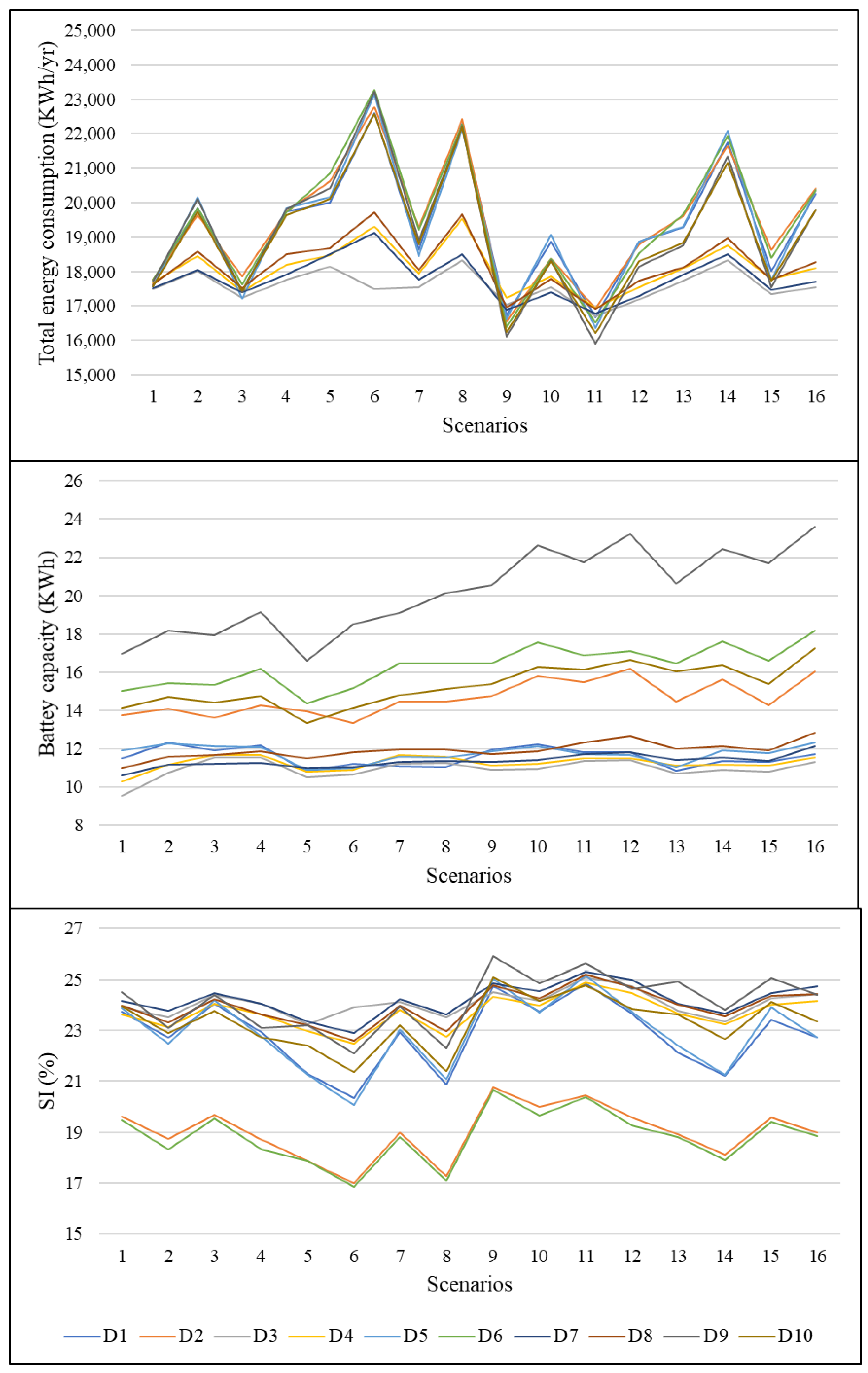
• For the suggested case study building, which meets the TEK17’s energy consumption target (110 kWh/m²), the cost-effective battery sizes for the different designs under the measured power rate tariff is in the range of 10-18 kWh. For the tiered rate tariff, the range is from 2 to 12 kWh, while, for the time of use tariff, the cost-effective battery size varies between 40 and 65 kWh.
• The higher sizes of the cost-effective batteries under the time of use tariff are related to the shifting strategy used in this tariff, which focuses on shifting the heating demand away from the daytime and needs higher capacities to store it.
• In the suggested design space, designs with weaker envelopes or exhaust ventilation in combination with an electric radiator have higher heating demands and higher heat peaks, thus leading to higher daily shifts and increases in the cost-effective battery size, as in designs $D_2$, $D_6$, $D_9$, and $D_{10}$. In contrast, designs using an ASHP can use smaller batteries to shift the heat under all of the tariffs due to less variation and smaller peaks in the heating demand.
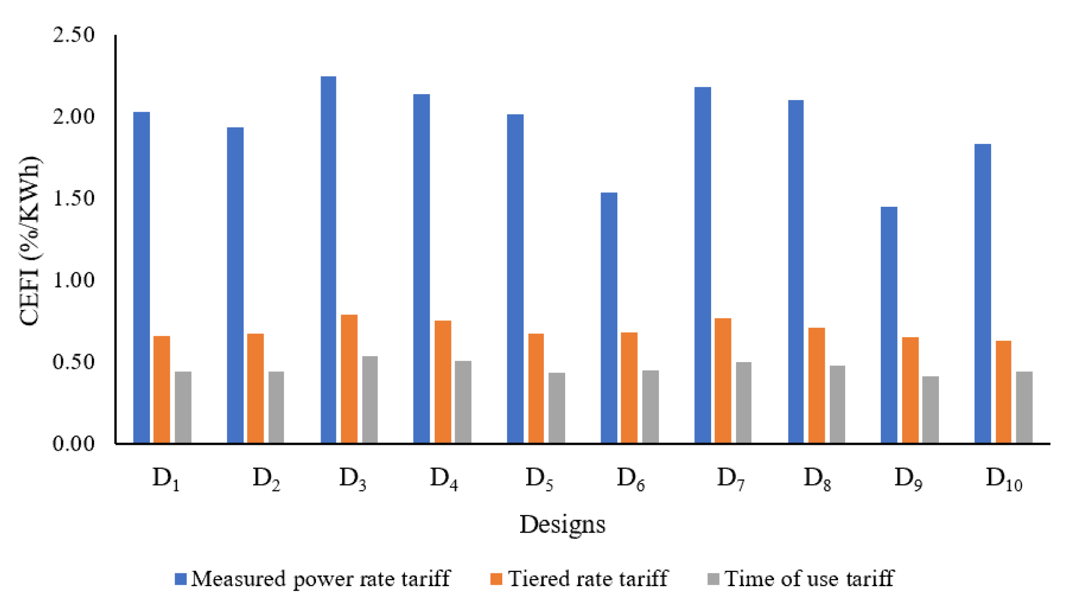
• When considering the three dynamic pricing tariffs, the highest CEFI is found for the measured power rate tariff, and its CEFI is significantly higher than those of the two other tariffs (1.4–2 %/kwh in comparison to 0.6–0.8 %/kWh for the tiered rate tariff and 0.4–0.55 %/kWh for the time of use tariff). In this tariff, neither the cost saving is as small as the tiered rate tariff, nor the battery capacity is as big as the time of use tariff.
• Of the ten designs with the same energy target, design $D_3$, which uses a combination of an electric radiator and ASHP as the energy system and air-balanced ventilation as the ventilation strategy, has the maximum CEFI of the designs. Thus, in this design space, ASHP and air-balanced ventilation are the most important design options for obtaining a high CEFI value. However, the implementation of renewable systems, which are paired with weak building envelopes to meet the energy target, or exhaust ventilation in combination with an electric radiator leads to lower CEFI values.
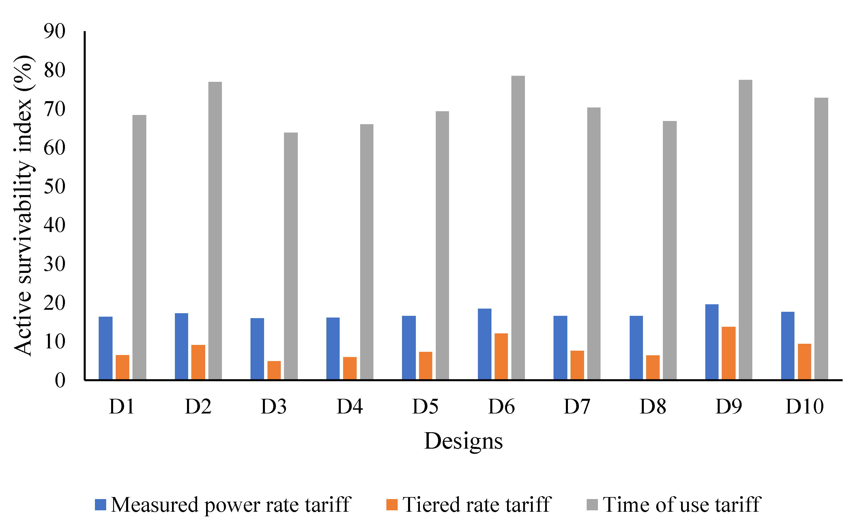
• For the case study building, which meets the TEK17’s energy consumption target (110 kWh/m²), the ASIs of the different designs under the time of use tariff vary between 63–80%. For the measured power rate tariff and tiered rate tariff, the ASI values decrease to 16–20% and 4–14%, respectively. The high active survivability under the time of use tariff is the result of a higher cost-effective battery size compared to the battery sizes for the other tariffs.
• Designs with higher cost-effective battery capacities can help the building survive longer during grid power failures. The ASI is higher in the designs with higher cost-effective battery sizes, such as designs $D_2$, $D_6$, $D_9$, and $D_{10}$.
• The building envelope and WWR are the most important parameters influencing passive survivability.
• There is a trade-off between the defined energy flexibility and survivability of the all-electric building for the three business models for the dynamic pricing tariff. The preferred design should be selected based on the prioritization of the criteria. Designs with an ASHP are suggested when the CEFI value is prioritized over the survivability in the case of power failure. In contrast, designs with higher battery capacities ($D_2$, $D_6$, $D_9$, $D_{10}$) are suggested when survivability is prioritized over energy flexibility.
• The CEFI and ASI values for the tiered rate tariff are more sensitive to weather and occupant uncertainties. For this tariff, the heat shift, the corresponded savings, and the cost-effective battery size depend on the selected subscription level, making it far more sensitive to uncertainties from the flexibility and active survivability points of view.

In the context of operational applicability, the suggested methodology can be used by the different stakeholders in building projects, such as grid companies, building designers, and electric grid customers, including home owners, to classify the energy flexibility and survivability of buildings according to two easy-to-understand indicators hinging on cost-effectiveness. The application of this methodology is not limited to Norway and can be extended to other countries where electricity is used as a heating source, such as Kosovo, Malta, Sweden, and Finland. Furthermore, it can be extended to countries with hot climates that use electricity for cooling. In this paper, the proposed methodology is considered for a single building. In the real world, buildings interact with each other and with connected grids. It would, therefore, be interesting to consider this approach on a larger scale, such as a neighborhood scale, by extending the sizing to centralized storage systems. The energy flexibility and survivability of buildings can also trade-off with other building performance metrics, such as energy consumption and emissions. In future work, energy flexibility and survivability can be used, along with other performance criteria, in a multi-criteria assessment framework to help decision-makers prioritize and select building designs.

References

1. Deason, J.; Wei, M.; Leventis, G.; Smith, S.; Schwartz, L. Energy Analysis and Environmental Impacts Division Lawrence Berkeley National Laboratory Electricity Markets and Policy Group; Technical Report; Lawrence Berkeley National Laboratory: Berkeley, CA, USA, 2018. [Google Scholar]
2. Lund, H.; Østergaard, P.A.; Connolly, D.; Ridjan, I.; Mathiesen, B.V.; Hvelplund, F.; Thellufsen, J.Z.; Sorknæs, P. Energy storage and smart energy systems. Int. J. Sustain. Energy Plan. Manag. 2016, 11, 3–14. [Google Scholar]
3. Clauß, J.; Stinner, S.; Solli, C.; Lindberg, K.B.; Madsen, H.; Georges, L. A generic methodology to evaluate hourly average CO2eq. In intensities of the electricity mix to deploy the energy flexibility potential of Norwegian buildings. In Proceedings of the 10th International Conference on System Simulation in Buildings, Liege, Belgium, 10–12 December 2018; pp. 10–12. [Google Scholar]
4. Persson, U.; Werner, S. Quantifying the Heating and Cooling Demand in Europe; Technical Report; Intelligent energy Europe program of the Europian Union: Halmstad, Sweden, 2018. [Google Scholar]
5. European Heat Pumps Association Website. Available online: https://www.ehpa.org/ (accessed on 8 October 2020).
6. International Energy Agency Website. Available online: https://www.iea.org/ (accessed on 8 October 2020).
7. Loibl, W.; Stollnberger, R.; Österreicher, D. Residential heat supply by waste-heat re-use: Sources, supply potential and demand coverage—A case study. Sustainability 2017, 9, 250. [Google Scholar] [CrossRef] [Green Version]
8. Clauß, J.; Stinner, S.; Sartori, I.; Georges, L. Predictive rule-based control to activate the energy flexibility of Norwegian residential buildings: Case of an air-source heat pump and direct electric heating. Appl. Energy 2019, 237, 500–518. [Google Scholar] [CrossRef]
9. Junker, R.G.; Azar, A.G.; Lopes, R.A.; Lindberg, K.B.; Reynders, G.; Relan, R.; Madsen, H. Characterizing the energy flexibility of buildings and districts. Appl. Energy 2018, 225, 175–182. [Google Scholar] [CrossRef]
10. Niu, J.; Tian, Z.; Lu, Y.; Zhao, H. Flexible dispatch of a building energy system using building thermal storage and battery energy storage. Appl. Energy 2019, 243, 274–287. [Google Scholar] [CrossRef]
11. Foteinaki, K.; Li, R.; Heller, A.; Rode, C. Heating system energy flexibility of low-energy residential buildings. Energy Build. 2018, 180, 95–108. [Google Scholar] [CrossRef]
12. Arteconi, A.; Mugnini, A.; Polonara, F. Energy flexible buildings: A methodology for rating the flexibility performance of buildings with electric heating and cooling systems. Appl. Energy 2019, 251, 113387. [Google Scholar] [CrossRef]
13. Statistics Norway. Available online: https://www.ssb.no/en/energi-og-industri/statistikker/elektrisitet/aar (accessed on 8 October 2020).
14. Bergesen, B.; Groth, L.H.; Langseth, B.; Magnussen, I.H.; Spilde, D.; Toutain, J.E.W. Energy Consumption 2012 Household Energy Consumption; Technical Report 16/2013; Norwegian Water Resources and Energy Directorate: Oslo, Norway, 2012. [Google Scholar]
15. Energy Consumption in Households. Available online: https://ec.europa.eu/eurostat/statistics-explained/index.php/Energy_consumption_in_households (accessed on 8 October 2020).
16. IEA. Global EV Outlook 2020; Technical Report; IEA: Paris, France, 2019. [Google Scholar]
17. Strbac, G. Demand side management: Benefits and challenges. Energy Policy 2008, 36, 4419–4426. [Google Scholar] [CrossRef]
18. Vandermeulen, A.; van der Heijde, B.; Helsen, L. Controlling district heating and cooling networks to unlock flexibility: A review. Energy 2018, 151, 103–115. [Google Scholar] [CrossRef]
19. Haider, H.T.; See, O.H.; Elmenreich, W. A review of residential demand response of smart grid. Renew. Sustain. Energy Rev. 2016, 59, 166–178. [Google Scholar] [CrossRef]
20. Shen, B.; Ghatikar, G.; Lei, Z.; Li, J.; Wikler, G.; Martin, P. The role of regulatory reforms, market changes, and technology development to make demand response a viable resource in meeting energy challenges. Appl. Energy 2014, 130, 814–823. [Google Scholar] [CrossRef]
21. Dutta, G.; Mitra, K. A literature review on dynamic pricing of electricity. J. Oper. Res. Soc. 2017, 68, 1131–1145. [Google Scholar] [CrossRef] [Green Version]
22. Gottwalt, S.; Ketter, W.; Block, C.; Collins, J.; Weinhardt, C. Demand side management—A simulation of household behavior under variable prices. Energy Policy 2011, 39, 8163–8174. [Google Scholar] [CrossRef]
23. Communication from the Commission to the European Parliament, the European Council, the Council, the European economic and social committee and the Committee of the Regions, the European Green Deal; Technical Report; European Commission: Brussels, Belgium, 2019.
24. Lund, P.D.; Lindgren, J.; Mikkola, J.; Salpakari, J. Review of energy system flexibility measures to enable high levels of variable renewable electricity. Renew. Sustain. Energy Rev. 2015, 45, 785–807. [Google Scholar] [CrossRef] [Green Version]
25. Schofield, J.; Carmichael, R.; Tindemans, S.; Woolf, M.; Bilton, M.; Strbac, G. Residential Consumer Responsiveness to Time-Varying Pricing; Technical Report A3; Low Carbon London Learning Lab, LCNF Project; Imperial College: London, UK, 2014. [Google Scholar]
26. Laicane, I.; Blumberga, D.; Blumberga, A.; Rosa, M. Reducing household electricity consumption through demand side management: The role of home appliance scheduling and peak load reduction. Energy Procedia 2015, 72, 222–229. [Google Scholar] [CrossRef] [Green Version]
27. Nezamoddini, N.; Wang, Y. Risk management and participation planning of electric vehicles in smart grids for demand response. Energy 2016, 116, 836–850. [Google Scholar] [CrossRef]
28. Moreau, A. Control Strategy for Domestic Water Heaters during Peak Periods and its Impact on the Demand for Electricity. Energy Procedia 2011, 12, 1074–1082. [Google Scholar] [CrossRef] [Green Version]
29. Mancini, F.; Nastasi, B. Energy retrofitting effects on the energy flexibility of dwellings. Energies 2019, 12, 2788. [Google Scholar] [CrossRef] [Green Version]
30. Chen, Y.; Xu, P.; Gu, J.; Schmidt, F.; Li, W. Measures to improve energy demand flexibility in buildings for demand response (DR): A review. Energy Build. 2018, 177, 125–139. [Google Scholar] [CrossRef]
31. Selinger-Lutz, O.; Groß, A.; Wille-Haussmann, B.; Wittwer, C. Dynamic feed-in tariffs with reduced complexity and their impact on the optimal operation of a combined heat and power plant. Int. J. Electr. Power Energy Syst. 2020, 118, 105770. [Google Scholar] [CrossRef]
32. Hamdy, M.; Sirén, K. A multi-aid optimization scheme for large-scale investigation of cost-optimality and energy performance of buildings. J. Build. Perform. Simul. 2016, 9, 411–430. [Google Scholar] [CrossRef]
33. Syed, M.; Hansen, P.; Morrison, G.M. Performance of a shared solar and battery storage system in an Australian apartment building. Energy Build. 2020, 225, 110321. [Google Scholar] [CrossRef]
34. Weniger, J.; Tjaden, T.; Quaschning, V. Sizing of Residential PV Battery Systems. Energy Procedia 2014, 46, 78–87. [Google Scholar] [CrossRef] [Green Version]
35. Hassan, A.S.; Cipcigan, L.; Jenkins, N. Optimal battery storage operation for PV systems with tariff incentives. Appl. Energy 2017, 203, 422–441. [Google Scholar] [CrossRef]
36. Heine, K.; Thatte, A.; Tabares-Velasco, P.C. A simulation approach to sizing batteries for integration with net-zero energy residential buildings. Renew. Energy 2019, 139, 176–185. [Google Scholar] [CrossRef]
37. Nastasi, B.; Mazzoni, S.; Groppi, D.; Romagnoli, A.; Garcia, D.A. Solar power-to-gas application to an island energy system. Renew. Energy 2021, 164, 1005–1016. [Google Scholar] [CrossRef]
38. Dumont, O.; Carmo, C.; Georges, E.; Balderrama, S.; Quoilin, S.; Lemort, V. Economic assessment of energy storage for load shifting in Positive Energy Building. Int. J. Energy Environ. Eng. 2017, 8, 25–35. [Google Scholar] [CrossRef] [Green Version]
39. Georgakarakos, A.D.; Mayfield, M.; Hathway, E.A. Battery Storage Systems in Smart Grid Optimised Buildings. Energy Procedia 2018, 151, 23–30. [Google Scholar] [CrossRef]
40. Yang, Y.; Li, H.; Aichhorn, A.; Zheng, J.; Greenleaf, M. Sizing strategy of distributed battery storage system with high penetration of photovoltaic for voltage regulation and peak load shaving. IEEE Trans. Smart Grid 2013, 5, 982–991. [Google Scholar] [CrossRef]
41. Prehoda, E.W.; Schelly, C.; Pearce, J.M. US strategic solar photovoltaic-powered microgrid deployment for enhanced national security. Renew. Sustain. Energy Rev. 2017, 78, 167–175. [Google Scholar] [CrossRef] [Green Version]
42. Tsianikas, S.; Zhou, J.; Birnie, D.P., III; Coit, D.W. Economic trends and comparisons for optimizing grid-outage resilient photovoltaic and battery systems. Appl. Energy 2019, 256, 113892. [Google Scholar] [CrossRef]
43. Ghasemieh, H.; Haverkort, B.R.; Jongerden, M.R.; Remke, A. Energy resilience modelling for smart houses. In Proceedings of the 2015 45th Annual IEEE/IFIP International Conference on Dependable Systems and Networks, Rio de Janeiro, Brazil, 22–25 June 2015; pp. 275–286. [Google Scholar]
44. Gupta, R.; Bruce-Konuah, A.; Howard, A. Achieving energy resilience through smart storage of solar electricity at dwelling and community level. Energy Build. 2019, 195, 1–15. [Google Scholar] [CrossRef]
45. UENTSO-E Overview of Transmission Tariffs in Europe: Synthesis. 2019. Available online: https://eepublicdownloads.blob.core.windows.net/public-cdn-container/clean-documents/mc-documents/190626_MC_TOP_7.2_TTO_Synthesis2019.pdf (accessed on 8 October 2020).
46. Sæle, H. Consequences for residential customers when changing from energy based to capacity based tariff structure in the distribution grid. In Proceedings of the 2017 IEEE Manchester PowerTech, Manchester, UK, 18–22 June 2017; pp. 1–6. [Google Scholar]
47. Sæle, H.; Høvik, Ø.; Nordgård, D.E. Evaluation of alternative network tariffs—For residential customers with hourly metering of electricity consumption. In Proceedings of the CIRED Workshop 2016, Helsinki, Finland, 14–15 June 2016. [Google Scholar]
48. Hansen, H.; Jonassen, T.; Løchen, K.; Mook, V. Høringsdokument nr 5-2017: Forslag til Endring i Forskrift om Kontroll av Nettvirksomhet; Technical Report; Norges Vassdrags—Ogenergidirektor: Oslo, Norway, 2017. [Google Scholar]
49. Smart metering (AMS). Available online: https://www.nve.no/energy-market-and-regulation/retail-market/smart-metering-ams/ (accessed on 8 October 2020).
50. Eriksen, A.B.; Hansen, H.; Hole, J.; Jonassen, T.; Mook, V.; Steinnes, S.; Varden, L. RME HoRINGSDOKUMENT, Endringer i Nettleiestrukturen; Norges Vassdrags-og Energidirektorat: Oslo, Norway, 2020. [Google Scholar]
51. Karlsen, S.S.; Hamdy, M.; Attia, S. Methodology to assess business models of dynamic pricing tariffs in all-electric houses. Energy Build. 2020, 207, 109586. [Google Scholar] [CrossRef]
52. EQUA Solutions AB Ida Indoor Climate and Energy (Version 4.8). Available online: https://www.equa.se/en/ida-ice (accessed on 8 October 2020).
53. Equa Simulation AB. Validation of IDA Indoor Climate and Energy 4.0 Build 4 with Respect to ANSI/ASHRAE Standard 140-2004. Technical Report. 2010. Available online: http://mail.ssf.scout.se/iceuser/validation/ASHRAE140-2004.pdf (accessed on 8 October 2020).
54. Equa Simulation AB. Validation of IDA Indoor Climate and Energy 4.0 with respect to CEN Standards EN 15255-2007 and EN 15265-2007. Technical Report. 2010. Available online: http://www.equaonline.com/iceuser/validation/CEN_VALIDATION_EN_15255_AND_15265.pdf (accessed on 8 October 2020).
55. MATLAB Version 9.3.0.713579 (R2017b); The Mathworks: Natick, MA, USA, 2017.
56. Rønneseth, Ø.; Haase, M.; Georges, L.; Thunshelle, K.; Holøs, S.B.; Fjellheim, Ø.; Mysen, M.; Thomsen, J. Building Service Solutions Suitable for Low Emission Urban Areas; Technical Report; The Research Center on Zero Emission Neighbourhoods (ZEN) in Smart Cities: Trondheim, Norway, 2020. [Google Scholar]
57. Immendoerfer, A.; Winkelmann, M.; Stelzer, V. Energy Solutions for Smart Cities and Communities Recommendations for Policy Makers from the 58 Pilots of the CONCERTO Initiativ; Technical Report; The Institute for Technology Assessment and Systems Analysis (ITAS) Karlsruhe Institute of Technology: Karlsruhe, Germany, 2014. [Google Scholar]
58. Wethal, U. Practices, provision and protest: Power outages in rural Norwegian households. Energy Res. Soc. Sci. 2020, 62, 101388. [Google Scholar] [CrossRef]
59. Reynders, G.; Lopes, R.A.; Marszal-Pomianowska, A.; Aelenei, D.; Martins, J.; Saelens, D. Energy flexible buildings: An evaluation of definitions and quantification methodologies applied to thermal storage. Energy Build. 2018, 166, 372–390. [Google Scholar] [CrossRef]
60. Oldewurtel, F.; Sturzenegger, D.; Andersson, G.; Morari, M.; Smith, R.S. Towards a standardized building assessment for demand response. In Proceedings of the 52nd IEEE Conference on Decision and Control, Firenze, Italy, 10–13 December 2013; pp. 7083–7088. [Google Scholar]
61. Baniassadi, A.; Sailor, D.J.; Krayenhoff, E.S.; Broadbent, A.M.; Georgescu, M. Passive survivability of buildings under changing urban climates across eight US cities. Environ. Res. Lett. 2019, 14, 074028. [Google Scholar] [CrossRef] [Green Version]
62. Ozkan, A.; Kesik, T.; Yilmaz, A.Z.; O’Brien, W. Development and visualization of time-based building energy performance metrics. Build. Res. Inf. 2019, 47, 493–517. [Google Scholar] [CrossRef]
63. O’Brien, W.; Bennet, I. Simulation-Based Evaluation of High-Rise Residential Building Thermal Resilience. ASHRAE Trans. 2016, 122, 455–468. [Google Scholar]
64. Byggteknisk Forskrift (TEK17). Available online: https://dibk.no/byggereglene/byggteknisk-forskrift-tek17/14/14-2/ (accessed on 8 October 2020).
65. Standard Norge (2016) SN/TS3031: 2016 Energy Performance of Buildings. Available online: https://www.standard.no/nyheter/nyhetsarkiv/bygg-anlegg-og-eiendom/2016/snts-30312016-for-beregning-av-energibehov-og-energiforsyning/ (accessed on 8 October 2020).
66. Rønneseth, Ø.; Sartori, I. Method for Modeling Norwegian Single-Family House in IDA ICE; Technical Report; The Research Center on Zero Emission Neighbourhoods (ZEN) in Smart Cities: Trondhiem, Norway, 2018. [Google Scholar]
67. Homaei, S.; Hamdy, M. A robustness-based decision making approach for multi-target high performance buildings under uncertain scenarios. Appl. Energy 2020, 267, 114868. [Google Scholar] [CrossRef]
68. Nord, N.; Qvistgaard, L.H.; Cao, G. Identifying key design parameters of the integrated energy system for a residential Zero Emission Building in Norway. Renew. Energy 2016, 87, 1076–1087. [Google Scholar] [CrossRef] [Green Version]
69. De Wilde, P.; Coley, D. The Implications of a Changing Climate for Buildings. Build. Environ. 2012, 55, 1–7. [Google Scholar] [CrossRef] [Green Version]
70. Hamdy, M.; Sirén, K.; Attia, S. Impact of financial assumptions on the cost optimality towards nearly zero energy buildings—A case study. Energy Build. 2017, 153, 421–438. [Google Scholar] [CrossRef] [Green Version]
71. Yan, D.; O’Brien, W.; Hong, T.; Feng, X.; Gunay, H.B.; Tahmasebi, F.; Mahdavi, A. Occupant behavior modeling for building performance simulation: Current state and future challenges. Energy Build. 2015, 107, 264–278. [Google Scholar] [CrossRef] [Green Version]
72. Hu, M.; Xiao, F. Quantifying uncertainty in the aggregate energy flexibility of high-rise residential building clusters considering stochastic occupancy and occupant behavior. Energy 2020, 194, 116838. [Google Scholar] [CrossRef]
73. Wang, A.; Li, R.; You, S. Development of a data driven approach to explore the energy flexibility potential of building clusters. Appl. Energy 2018, 232, 89–100. [Google Scholar] [CrossRef]
Figure 1. The conceptual framework of the study.
Energies 14 02787 g001
Figure 2. Illustration of: (a) Energy rate tariff, (b) measured power rate tariff, (c) tiered rate tariff, and (d) time of use tariff in typical winter and summer days. The illustration shows hourly loads over 24 h for the example single-family house. The penalized hours in each tariff are shown in red.
Energies 14 02787 g002
Figure 3. Flow diagram of the algorithm developed in MATLAB.
Energies 14 02787 g003
Figure 4. The winter load profiles for the ideal heat shifts of different business models of dynamic pricing tariffs.
Energies 14 02787 g004
Figure 5. Illustration of determining the cost-effective battery sizing for a typical building.
Energies 14 02787 g005
Figure 6. Layout and appearance of a representative single-family house with a floor area of 162 m2.
Energies 14 02787 g006
Figure 7. Annual costs (before and after shifts) and effective shifts for the ten designs across 16 scenarios and the different tariffs.
Energies 14 02787 g007
Figure 8. A comparison of the daily shifts for D 2 , D 6 , and D 1 under the measured power rate tariff.
Energies 14 02787 g008
Figure 9. Visualization of designs based on SI, cost-effective battery size, and daily ideal shift (a) The relationship between the SI and cost-effective battery size. (b) The violin plots of the daily shifts for the ten designs in the reference scenario.
Energies 14 02787 g009
Figure 10. The CEFI values for the ten designs in the reference scenario and three tariffs.
Energies 14 02787 g010
Figure 11. Winter passive survivability performances of the ten designs following a grid power outage in the winter.
Energies 14 02787 g011
Figure 12. Active survivability indexes for the ten designs in the reference scenarios and three business models of dynamic pricing tariff.
Energies 14 02787 g012
Figure 13. The trade-offs between cost-effective energy flexibility and survivability. The bubble size indicates the relative value of passive survivability index.
Energies 14 02787 g013
Figure 14. The uncertainties related to the CEFIs and ASIs for the three business models of dynamic pricing tariff.
Energies 14 02787 g014