Abstract
Reliable seismic hazard analyses are crucial to mitigate seismic risk. When dealing with induced seismicity the standard Probabilistic Seismic Hazard Analysis (PSHA) has to be modified because of the peculiar characteristics of the induced events. In particular, the relative shallow depths, small magnitude, a correlation with field operations, and eventually non-Poisson recurrence time. In addition to the well-known problem of estimating the maximum expected magnitude, it is important to take into account how the industrial field operations affect the temporal and spatial distribution of the earthquakes. In fact, during specific stages of the project the seismicity may be hard to be modelled as a Poisson process—as usually done in the standard PSHA—and can cluster near the well or migrate toward hazardous known or—even worse—not known faults. Here we present a technique in which we modify the standard PSHA to compute time-dependent seismic hazard. The technique allows using non-Poisson models (BPT, Weibull, gamma and ETAS) whose parameters are fitted using the seismicity record during distinct stages of the field operations. As a test case, the procedure has been implemented by using data recorded at St. Gallen deep geothermal field, Switzerland, during fluid injection. The results suggest that seismic hazard analyses, using appropriate recurrence model, ground motion predictive equations, and maximum magnitude allow the expected ground-motion to be reliably predicted in the study area. The predictions can support site managers to decide how to proceed with the project avoiding adverse consequences.
1. Introduction
Mitigation of seismic risk basically depends on the reliability of seismic hazard analysis. When dealing with induced seismicity, however, standard approaches, such as Probabilistic Seismic Hazard Analysis (PSHA) e.g., [1,2] cannot be applied as they have been originally conceived. They need to be modified to consider the specific features of the induced seismicity e.g., [3,4,5]. The main differences are related to both temporal and spatial distribution of the induced seismicity compared to natural seismicity. Indeed, induced seismicity tends to cluster in limited volumes near the wells where field operations (e.g., fluids injection, extraction, fracking, etc.) are performed. From a temporal point of view, earthquake occurrence, in some cases, may be not stationary over small time-windows such as the extent of the geoengineering project (e.g., [5,6,7,8]). Hence, the homogeneous Poisson recurrence model can be used under some assumptions that can impact the final hazard estimates. In the context of the induced seismicity, non-Poisson models have been proposed, for example, by Langenbruch et al. [6] who considered the generalized Poisson model in which the process intensity (i.e., earthquakes frequency) is not constant and can vary with time. Bachmann et al. [7] used the Reasenberg and Jones Epidemic Type Aftershock Sequence (ETAS) models e.g., [9]. Baker and Gupta [10] used a gamma distribution in a Bayesian updating approach for seismic hazard. Broccardo et al. [11] integrated the approach proposed by Mignan et al. [12] in a hierarchical Bayesian modelling, which relates the seismicity rate of a non-homogeneous Poisson process to the injection flowrate.
Furthermore, the magnitude of induced events generally ranges in tighter intervals with respect to natural seismicity. In this regard, one of the most challenging questions is the identification of the expected maximum magnitude to be used in the hazard computation e.g., [13,14,15].
Finally, as noted by Van Eck et al. [16], due to the extent of the catalogues and in general of the duration of Enhanced Geothermal Systems (EGSs) operations the exposure and return periods to be considered have to be different from those used in standard PSHA.
In the present study we propose a technique aimed at facing the above-mentioned modifications of the standard PSHA. Following the approach proposed by Convertito and Zollo [17] and modified by Convertito et al. [5], we use data—events’ location and peak-ground velocities (PGVs)—collected during a specific phase of a project, to define a proper seismogenic volume, the maximum magnitude and, through the analysis of the inter-arrival times distribution, the recurrence model. This latter can then be used to perform a time-independent or a time-dependent seismic hazard analysis by considering specific probability density functions to compute the seismicity rate. The study also implements the ETAS model to obtain time-dependent rates of exceedance of PGV values and compares the results both to the time-dependent and time-independent seismic hazard assessments.
With the aim of testing if and how the proposed approach predicts what should be observed as a consequence of the current field operations, we compare the estimated PGV values for selected probabilities of exceedance, with the observed values. The procedure has been implemented by using data recorded at St. Gallen (Switzerland) deep geothermal field during fluid injection. The network managed by Swiss Seismological Service (SED; [18,19]) originally consisted of one short period borehole sensor at 205 m depth and five additional broadband surface stations operated within a 12 km radius around the borehole. In July 2103 the network was additionally densified with seven short period surface stations [20]. Overall, the data analyzed in the present study were recorded by 10 stations (Figure 1).
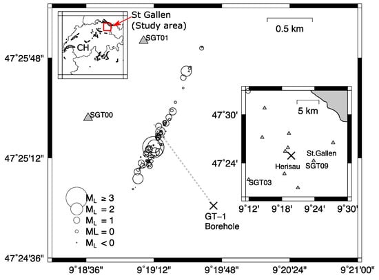
Figure 1.
Plan view of the analyzed earthquakes. Circles representing earthquakes location are proportional to the magnitude of the event. Seismic network layout is indicated in the right bottom frame where the location of the two nearest urban areas from the well and the two sites (SGT03 and SGT09) selected for site-specific seismic hazard analysis is also indicated. The grey dashed line indicates the GT-1 well trajectory. The upper left inset indicates the location of the St Gallen study area in Switzerland.
The target of the project was a carbonate aquifer at a depth of 4 km b.s.l. to produce electricity and heating. As described by Moeck et al. [21] and Zbinden et al. [22], the project started with a stimulation phase on 14 July 2013. Water was injected at about 3.6 km depth b.s.l, at a rate of 53 L/s for a total amount of 175 m3 in 2 hrs. During the stimulation phase only microseismicity with magnitude lower than 0.2 was induced. From 14 July 2013 through 19 July 2013 acid stimulations were performed involving about 290 m3 of fluids, which broke seal to gas reservoir and caused a gas kick (95% CH4). Afterwards, well control operations were done by injecting ~700 m3 of water and heavier liquids, which probably induced the largest event in the sequence with ML 3.5. Well control operations ended on 24 July 2013. Despite this adverse consequence, in August 2013 a decision was made to continue the field operations with a high feeling of solidarity from the public. In September 2013 fishing operations (that is removing lost or stuck objects from the wellbore) were done together with a cleaning of the well [21]. As reported by Diehl et al. [20], overall, the induced seismic sequence counted 346 locatable events with magnitude in the range (−1.2, 3.5) and depths ranging between 4.4 and 4.7 km (Figure 2).
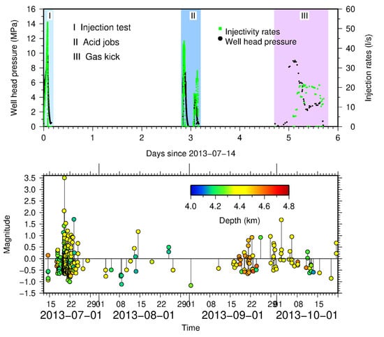
Figure 2.
Upper panel: well head pressure (black dots) and injectivity rates (green dots) during the different phases of the project as reported by Moeck et al. [21]. Lower panel: temporal evolution of seismicity from 2013-07-14 to 2013-10-22. Earthquakes are color coded according to the depth.
Similar to almost all the statistical approaches [5,7], our approach does not directly deal with the details of the physics of the ongoing processes that are inducing earthquakes. It focuses on the possibility of predicting the expected ground-motion levels in proper calibrated future time windows. Specifically, for distinct stages of the project, we compare observed PGVs at two sites with predictions obtained selecting the best fitting probability density function on inter-arrival times with respect to the standard Poisson process. Moreover, we propose not only to employ specific recurrence models but also to use updated ground motion prediction equations (GMPEs) when new and more robust data are being collected [23,24,25]. This is a critical issue, indeed, for several aspects: (i) the range of magnitude of induced seismicity, in general, is not covered by GMPEs developed by using strong-motion data; (ii) empirical ground motion relations may not work well when source-to-site distances are small (aka. the “near source” issue); (iii) the fact that field operations may produce time dependent variations in the propagation medium and seismic source properties that can modify the observed peak-ground motion values and should be thus included in the GMPEs e.g., [25]. Finally, taking into account for the timescale is particularly important since, as noted by Baish et al. [26], the most hazardous events frequently occur post-injection. Thus, decisions on reducing/stopping or continuing field operations should not be based solely on what is currently observed but also on what is expected.
2. Method
In order to estimate seismic hazard for induced earthquakes, by considering their main features, that is, relative shallow depths, small magnitude, a dependence on the field operations, and eventually non-Poisson recurrence time, we implement some modifications to the standard hazard integral formulation. For a point source, the hazard integral leads to the frequency of exceeding a given reference value of the selected ground motion parameter and its general formulation is as it follows (e.g., [1,2]):
where I[.] is an indicator function, which equals 1 if A is larger than a given reference value for a given distance r, a given magnitude m, and a given ε. As for distance and magnitude, a minimum and a maximum value must be defined based on a-priori information (e.g., the minimum damaging magnitude value, the maximum expected magnitude value, the relative source-to-site distance). The variable ε represents the residual deviation of the A parameter related to the median value provided by the selected GMPE e.g., [27,28]. By definition it corresponds to the number of logarithmic standard deviations by which the the ground motion deviates from the mean on a logscale. The associated probability density function (PDF), f(), is assumed to be the normal PDF e.g., [27].
The PDF for m, f(m), depends on the selected earthquake recurrence model whereas the PDF for the distance r, f(r), depends on the source geometry and position of site. The parameter is the mean annual rate of occurrence of the earthquakes having magnitude larger than the cut-off magnitude Mct for each selected source zone and is estimated by analysing the earthquake catalogues or by adopting spatio-temporal seismicity models like ETAS.
Assuming that, for a given site, the event A > is a selective process and that seismicity is stationary (or piece-wise stationary for non-homogenous Poisson processes) with rate , for a given time-interval t, Equation (1) allows to compute the probability of exceedance P as:
where N the number of the sources that contribute to the hazard. When the analysis is done for a set of sites in an area of interest for selected values of the exposure time and the probability of exceedance, a hazard map can be obtained [29,30].
In this study, we propose a specific formulation for the PDF of distance, and a technique to estimate the expected maximum magnitude and to compute the mean annual rate of occurrence. In particular, we identify a proper recurrence model from the analysis of the inter-arrival times distribution and adaptively fit a spatio-temporal ETAS model (e.g., [31,32,33]) to the catalogue of induced earthquakes.
Moreover, to compute the indicator function in Equation (1), as found by De Matteis and Convertito [23] and Convertito et al. [25], we assume that also GMPEs should be recalibrated to account for the medium propagation and source variations produced during the field operations. To this aim, for each phase of the geo-energy project, we infer a specific GMPE. Next, through an F-test, we verify if it can be used instead of the previous model or this latter can be still used.
As for the PDF of distance fR(r), we use the hypocentral distance as distance metric and use a volume seismogenic source instead of an aerial source. In particular, we cover the entire volume of interest by a 3D grid and, among all the elementary volumes, we consider only those containing at least one earthquake. A possible advantage is that the seismogenic potential is not fixed a-priori but can evolve during the geo-energy project.
Several techniques are available to estimate the maximum magnitude value to be used for seismic hazard analysis. They can be based on information about current field operations (e.g., injected volumes, shape and extent of the seismicity cloud, etc.) as those proposed by McGarr [15] or Shapiro et al. [14] or can be purely statistical approach. The latter approach comprises those proposed by Kijko [34] and Kijko and Singh [35].
While the techniques proposed by McGarr [15] or Shapiro et al. [14] can be used if the required information are available or planned for the future, those proposed by Kijko [34] and Kijko and Singh [35] requires data inversion procedures that cannot be enough stable when applied to events with magnitude in a limited range. In addition to the previous techniques, in the present study, we propose an approach that is based only on the current recorded seismicity and an assumed a-priori value of probability of exceeding some magnitude threshold. We provide an analytic expression that can be used in near real time approaches. In particular, we aim at computing the conditional probability:
which corresponds to the probability that the maximum magnitude, , is larger than a given value M* (between and given that the current observed largest observed magnitude in the catalogue is , and that overall the magnitude it is not expected to be larger than . If one assumes that the PDF on magnitude is a lower truncated exponential PDF, it can be demonstrated that the above conditional probability results in:
Thus, for a set of M* values, it is possible to compute the probability that they are not exceeded. Finally, the value assumed as can be the value that is not exceed at a selected probability value (e.g., 80%, 90%, 95%…).
Lastly, in order to account for non-Poisson nature of the induced seismicity, we propose to analyse the inter-arrival times distribution of the current seismicity, and to test it against several PDFs generally used to model the recurrence models with memory e.g., [36,37,38,39,40]. Particularly, in addition to the exponential PDF (corresponding to the Poisson recurrence model) we use the Brownian Passage Time model [41], the Weibull PDF, the Gamma PDF, and the Gaussian PDF. For each period, given that a sufficient number of events is available, we use the Kolmogorov-Smirnov test to infer the best fit PDF. Once the best PDF has been obtained, following Petersen et al. [42], we compute the equivalent annual rate r = −ln(1 − P)/t. The parameter P is the time-dependent probability of interest, which corresponds to the conditional time-dependent probability of having an event in a specified time interval —corresponding to the selected exposure time t that can be used in the hazard integral—given that the time te when the last event has occurred is known. P is given by:
The equivalent rate r of exceeding the cut-off magnitude is then substituted by in Equation (1). Furthermore, a spatio-temporal epidemiological model of the ETAS family (e.g., [31,32,33]) is used to predict the daily rate of exceeding the cut-off magnitude assuming a non-homogenous Poisson process for the inter-arrival times. In such a model, the process is assumed to be piece-wise stationary in the forecasting interval (e.g., here assumed to be 24 h). For a given forecasting interval, the seismicity rate in Equation (1) can be estimated with expected value of N(m|seq,Mct). The latter represents the number of events having magnitude equal to or larger than m, M ≥ m, conditioned to the sequence of previous events (denoted as seq including the events up to the starting time of the forecasting interval) and lower cut-off magnitude Mct. Assuming that the horizontal projection A of the seismogenic volume is divided into cell units Ai with centroids (xi, yi), the expected value E[N(m|seq,Mct)] can be estimated from the following equation:
where E[N(xi,yi,m|seq,Mct)] is the expected value of the conditional number of earthquakes with M ≥ m occurred in the cell unit with centroid (xi,yi). A robust estimate [43,44,45,46] of N(xi,yi,m|seq,Mct) can be obtained by integrating over the domain of the ETAS model parameters:
where p(θ |seq, Mct) is the conditional joint PDF for ETAS model parameters θ given the seq and the lower cut-off magnitude Mct; Nb(xi,yi,m|Mct) is the contribution of background seismicity to the number of events with M ≥ m for the ith; is the rate of occurrence of events in the forecasting interval [Tstart, Tend] (e.g., one day here) at time t (since an arbitrary time reference) with the time of origin at To, having M ≥ m, and occurring in the cell unit centered at (xi, yi)∈A. The rate is conditioned on the observation history seq, which is the sequence of No events taken place before the forecasting interval, i.e., in the interval [To, Tstart) and the lower cut-off magnitude Mct. That is, seq can be expressed as seq = {(tj, xj, yj, mj), To ≤ tj <Tstart, mj ≥ Mct, j = 1:No}, where tj is the arrival time of the j-th event with magnitude mj and location (xj, yj)∈A. The rate is expressed as a function of vector θ = [b, K, a, c, p, d, q, Kt, Kr] of ETAS model parameters:
The integral in Equation (7) over the domain of model parameters θ is solved numerically by using an adaptive Markov Chain Monte Carlo Simulation (MCMC) procedure (see [45,46,47] for more details).
3. Data Analysis and Results
Data analyzed in this study have been collected by Swiss Seismological Service in 2013 (from 2013-07-14 to 2013-10-22) during the well control measures after drilling and acidizing the GT-1 well (see Figure 1). The project started on 14 July 2013 with a stimulation phase during which a test of injection with flow rates of up to 53 l/s was performed. The resulting maximum pressure increase was 9.8 MPa e.g., [21,22]. For this phase 175 m3 of water were injected into the reservoir over a 2 h period. On 17 July 2013, an acid stimulation was performed with a 290 m3 of fluid injected. Well head pressure and injectivity rates during different phases of the project as reported by Moeck et al. [21] are shown in Figure 2 together with the temporal evolution of seismicity.
Overall, the induced seismicity counts 346 earthquakes with magnitude (ML) in the range (−1.2, 3.5) and depth ranging between 4.4 and 4.7 km. Events’ location corresponds to the double-difference location provided by Diehl et al. [20]. Three component recordings (sampled at 200 Hz) are available at 10 stations (Figure 1).
Based on the temporal evolution of the seismicity, we divide the whole catalogue in six different periods or phases whose duration is listed in Table 1. The selection criterion is subjective but guarantees that at least 20 events for each phase of the project are available to infer GMPE coefficients and the best inter-event PDF.

Table 1.
Inferred coefficients together with the uncertainty of the GMPE by using data relative to the considered phases of the project. The duration of each phase is listed in the second column. Nd indicates the number of used PGVs. F-value is the value of the statistic used in the F-test and is governed by the Fisher distribution. Prob is the probability of finding an F-value equal or larger than the one observed value in the assumption that the null hypothesis (Ho: No difference in variances between old and new model) is true. More specifically, the probability that the obtained results could have happened by chance. Probabilities in bold indicate that the new inferred model can be used instead of the previous one. As for phase 1, the current model is compared with the reference model reported in Equation (10).
With the aim of evaluating the prediction capabilities of the proposed technique, when inferring the GMPE, we do not consider PGVs recorded at stations SGT03 and SGT09, which are located at different distance (about 11 km and 5 km, respectively) and azimuth with respect to the injection well location (Figure 1). The PGVs at these two selected stations are used to compare the observed data with the predictions of the computed seismic hazard analysis at different probability of exceedance.
As for the GMPE we use the following formulation:
where PGV is in m/s, M is the magnitude (corresponding to ML here), R is the hypocentral distance in km. The GMPE is also associated with a logarithmic standard deviation σlnPGV corresponding to the total standard error, describing uncertainty in the value of lnPGV given the predictive relationship. Original waveforms are band-pass filtered (using a 4-poles Butterworth filter) in the range 2–90 Hz. The PGV correspond to the vector composition of the maximum value measured on the three components. The coefficients of the GMPE have been inferred by using the Levenberg–Marquardt least squares algorithm [48].
Since for the first phase of the project the number of recorded events could not be enough, we consider two options: (i) using a GMPE obtained from previous studies in the zone (as close and similar as possible in terms of tectonic regime) where the project is going to be developed; (ii) using a GMPE inferred from similar projects but in different areas. For the present study we use as reference model the GMPE proposed by Douglas et al. [49], which has been inferred by analyzing data recorded in several geothermal areas and spanning similar magnitude and distance ranges as those considered in our application. The corresponding equation is:
where PGV is in m/s, R is the hypocentral distance expressed in km, is the magnitude, and the total standard error is σlnPGV = 1.863.
Thus, using data from the first phase of the project we infer the parameters of Equation (9) and test if the model can be used instead of the GMPE in Equation (10). We assume that the current GMPE model can be used if it passes a one-side F-test at 95% level of confidence, that is, if the updated model has a statistically significant lower variance with respect to the previous model (see Table 1).
The PGVs as function of the distance are depicted in Figure 3 together with the GMPEs.
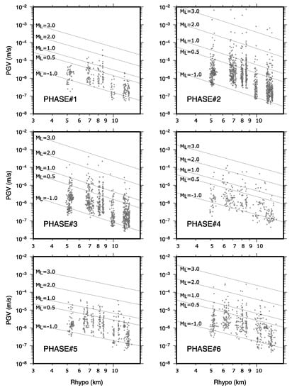
Figure 3.
Peak-ground velocities (PGVs) as function of the hypocentral distance for each of the six phases of the project analyzed in the present study. In each panel, the continuous lines refer to the GMPEs whose coefficients are listed in Table 1 evaluated for = −1.0, 0.5, 1.0, 2.0 and 3.0.
Table 1 contains the number of available PGVs for the specific period, the inferred coefficients (together with the uncertainties), the total standard deviation, the F-value (i.e., the value of the statistic used in the F-test) and the corresponding probability. This latter is the probability of finding an F-value equal or larger than the one observed value in the assumption that the null hypothesis (Ho: No difference in variances between old and new model) is true. For each phase, we estimate the minimum magnitude of completeness (Mc) by using the maximum curvature approach [50]. The results are listed in Table 2.
Table 2.
Minimum magnitude of completeness (Mc), b-value, maximum magnitude and the best fit PDF for the analyzed periods. Concerning the values in parenthesis are obtained by using the approach proposed by McGarr [15]. For the second period, we report three different estimates since two distinct operations were done involving 290 m3 and 700 m3 of injected fluids, respectively. The first number in parenthesis is the magnitude corresponding to the first volume 290 m3, the second to the 700 m3 volume, and the third to sum of the volumes (990 m3). corresponds to the observed maximum magnitude in each phase.
The b-value is computed by using the maximum likelihood formulation [51] and the associated uncertainty by using the Shi and Bolt [52] approach (see Table 2). The maximum magnitude to be use in the hazard integral is computed by using Equation (4) by selecting 90% as the probability of not being exceeded and arbitrarily setting = 5.0. This is in accordance with the observation that two historic earthquakes of Mw ≥ 4.0 have been reported in the seismogenic volume considered in the present study e.g., [53]. The resulting values for each phase are listed in Table 2. For two specific cases, for which the total injected volume is known, they are compared with the value obtained by using the approach proposed by McGarr [15]. In particular, we compute the maximum scalar seismic moment using the equation = G∆V where ∆V is the injected volume in m3 and G = 3e+10 Pa is the shear modulus. Next, we convert the seismic moment in moment magnitude using the Hanks and Kanamori [54] relationship. The results suggest that the McGarr [15] approach provides maximum magnitude values that are lower than the actual observed value corresponding to 3.5.
As for the inter-arrival time distribution, we aim at identifying the best recurrence model on the basis of the ongoing evolution of the seismicity. For each phase of the project, we test the Poisson model, the Brownian Passage Time model [42], the Weibull PDF, and the gamma PDF. The best model is identified by using the Kolmogorov-Smirnov test and is listed in Table 2. Once the best PDF has been obtained, following Petersen et al. [42] we compute the equivalent annual rate r = −ln(1 − P)/t, where P (see Equation (5)) is the time-dependent probability of interest in the selected exposure time t that can be used in the hazard integral. Figure 4 shows the fit of the inter-arrival times for phase 2 and phase 5 (see Table 1 for the specific time periods).
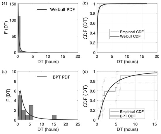
Figure 4.
Inter-arrival times distribution. The left column reports the distribution (in terms of frequency F) of the inter-arrival times DT. Panels (a) and (c) correspond to the phase 2 and phase 4, respectively. The black line depicts the best fit distribution, which corresponds to the Weibull PDF in panel (a) and to the Brownian Passage time PDF in panel (b). Panels (c) and (d) show the cumulative distribution used for the Kolmogorov-Smirnov test. The dashed lines represent the confidence bound.
As for the ETAS model, using Equation (7) we compute the expected daily rate of events having magnitude greater than the cut-off magnitude Mct = −0.5, which corresponds to the mean magnitude of completeness of the six phases of the project (Table 2), in the period starting from first forecast interval: 2013-07-20–6:00 A.M.–2013-07-21 6:00 A.M. (24 h) to the last forecast: 2013-10-22–6:00 A.M.–2013-10-23 6:00 A.M. (24 h). The results are shown in Figure 5 and indicate that the forecast capability of the model increases with time, that is, with the increasing number of recorded earthquakes. In addition to the temporal comparison, we also compare observed and predicted spatial distribution of the seismicity. In Figure 6, for three forecasting periods, we report the maps at 98% confidence interval for the number of earthquakes per cell units (latitude/longitude cells of a 0.001°× 0.001°) with ML ≥ Mct = −0.5, for 24 h forecasting intervals.
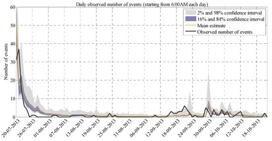
Figure 5.
The statistics of the daily number of events having magnitude greater than the cut-off magnitude N(m ≥ Mct|seq,Mct), Mct = −0.5 in the period starting from first forecast interval: 2013-07-20 6:00 A.M.–2013-07-21 6:00 A.M. (24 h) to the last forecast: 2013-10-22 6:00 A.M.–2013-10-23 6:00 A.M. (24 h). The statistics are represented by the 2nd–98th (grey area) percentiles and 16th–84th (blue area) percentiles confidence intervals and the mean (expected value from Equation (5)). The reference time is To = 2013-07-14 at 12:00. The evolution of the observed number of events is shown with black-solid line.
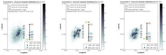
Figure 6.
Forecasted versus observed seismicity distribution, the maps report the 98% confidence interval for the number of earthquakes per cell units (latitude/longitude cells of a 0.001°× 0.001° grid) with ML ≥ Mc = −0.5, for 24 h forecasting intervals: (left) interval [Tstart = 2013-07-20, Tend = 2013-07-21]; (center) interval [Tstart = 2013-07-21, Tend = 2013-07-22]; (right) interval [Tstart = 2013-07-22, Tend = 2013-07-23]; The reference time interval is To = 2013-07-14 at 12:00 UTC (the first event of the catalog occurred about 6 min after the reference time To). The observed (green star) vs. the error-bar is also shown for each sub-figure. The error bar is shown with the forecasted median value (the 50th percentile) labeled with a grey-filled square, the forecasted 16th and 84th percentiles (blue numbers), and the forecasted 2nd and 98th percentiles (red numbers).
Figure 6 depicts the seismic events of interest that occurred in the corresponding forecasting interval [Tstart, Tend], shown as colored squares and dots (distinguished by their magnitudes). The results in Figure 6 indicate that the ETAS model captures properly the spatial distribution of seismic events taken place in the forecasting time interval. Inside each sub-figure of Figure 6, the observed (shown as a green star) vs. forecasted number of events (shown in an error-bar format) is illustrated for events with M ≥ Mct = −0.5 for the entire zone of seismic activities. It is to note that to retrospectively perform robust seismicity forecasting within the seismic sequence, we set Mct = −0.50 to be consistent with Table 2. However, this assignment has been verified based on the two procedures adopted for evaluating the completeness magnitude within a seismic sequence in the Electronic Supplementary Information in Ebrahimian and Jalayer [46].
The error-bar for the forecasted number of events features: the median value (the 50th percentile, equivalent of the logarithmic mean in the arithmetic scale) marked with a grey-filled square; the (logarithmic) mean plus/minus one (logarithmic) standard deviation indicating the interval between 16th and 84th percentiles (marked with blue horizontal lines and numbered in blue); the (logarithmic) mean plus/minus two (logarithmic) standard deviations indicating the interval between 2nd and 98th percentiles (marked with black horizontal lines and numbered in red). This is done to help in locating the observed number of events (marked and numbered in green) within plus or minus certain number of standard deviations from the mean estimate. It can be seen that observed number of events is captured properly with respect to plus/minus two standard deviation of the mean estimate.
We compute seismic hazard, expressed as PGV corresponding to given probability of exceedance levels at two selected stations SGT03 and SGT09 (see Figure 1). We considered three probability of exceedance levels: 10%, 20% and 50% and three exposure periods 15 days, 1 month and 2 months compatible with the duration of the project. We compare the results obtained by using the standard Poisson model, the model inferred for each phase, and the ETAS model. As for ETAS, in order to be consistent with the selected exposure times, we use the mean daily forecasted seismicity to compute the monthly rate. The recorded PGVs as function of the time at the two selected stations are shown in Figure 7, Figure 8 and Figure 9 for exposure times of 15 days, 1 month and 2 months, respectively. The figures demonstrate that in some of the considered periods the recorded values tend to 5 mm/s for which damage to ordinary buildings is deemed possible [55]. The PGV values obtained from the hazard analysis together with the associated probability of exceedance are shown as horizontal lines.
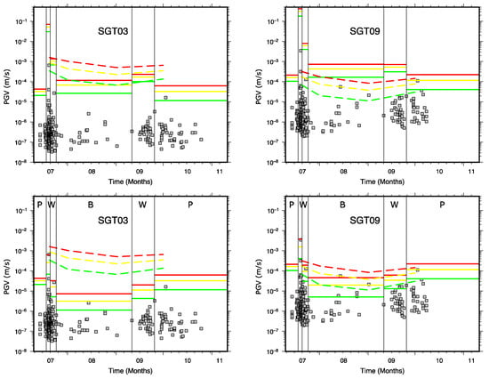
Figure 7.
Hazard analysis for three probability of exceedance (10% (red line), 20% (yellow) and 50% (green)) and a 0.5 month exposure time. The same color code is used for the ETAS model, but with dashed lines. The time period is reported in Table 1. Upper panels refer to time independent analysis while lower panels refer to the time dependent analysis. Letters in the lower panels indicate the best PDF for each period (P: Poisson; W: Weibull; B: Brownian Passage Time) (See Table 1). Grey squares represent the observed PGVs at the two stations indicated in the two panels.
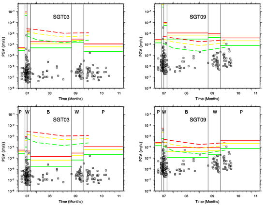
Figure 8.
Same as Figure 7, but for 1.0 month exposure time.
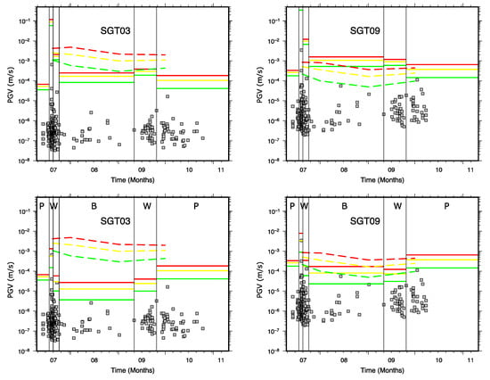
Figure 9.
Same as Figure 7, but for 2.0 month exposure time.
The results indicate that using a time-dependent model provides a more robust control on the expected PGV values. In particular, the use of the Weibull PDF and the BPT PDF, together with updated GMPEs provide predictions closer to the observed PGV values. Contrarily, the PGV values estimated by using the Poisson model seems to overestimate the observed PGV values leading to overpredict the associated hazard.
As for the time independent analysis, the ETAS model performs better than the Poisson model at station SGT09 and provides hazard estimates close—and even better in the second period—to the Weibull model and BPT model. On the other hand, for the station STG03, which is located at a larger distance with respect to SGT09, ETAS provides an overestimation of the hazard. This is probably indicating that the distance kernel used for predicting the spatio-temporal clustering of aftershocks (characterized by two parameters d and q in Equation (8)) is not steep enough for induced seismicity. This aspect has to be further investigated by testing other function forms as the distance kernel.
4. Conclusions
We present a technique aimed at modifying the standard probabilistic seismic hazard analysis when applied to induced seismicity. In particular, concerning the probability density function of distance fR(r), we use the hypocentral distance as distance metric and use a volume seismogenic source whose shape is modified according to the current seismicity spatial distribution, instead of a seismogenic source area. Moreover, we propose a technique for estimating the expected maximum magnitude value, which use the current probability density function on magnitude, that is, the Gutenberg-Richter relation and prior information about long-term seismicity. However, the most relevant modifications are two. The first one concerns the idea of updating the ground motion prediction equation during the distinct phases of the project while new and more robust PGVs data are recorded. The second is to test whether non-Poisson models, which assumes that successively occurring events are not causally related to each other, provides a better fit of the observed inter-arrival times distribution with respect to the Poisson model used in the standard PSHA. This is indeed a critical point when dealing with induced seismicity e.g., [5,7,8,11]. For the application presented in this study and concerning the St Gallen geothermal project in Switzerland, in addition to the Poisson model, we test Weibull PDF, gamma PDF, and BPT model. The use of the Kolmogorov-Smirnov test indicates that, in most of the phases of the project, the inter-arrival times distribution is not exponential, that is, the recurrence model is not Poisson. Moreover, we implement a robust framework by employing ETAS seismicity model [46,47] that allows to forecast both the temporal and spatial seismicity distribution. The capability of forecasting the spatial distribution of the seismicity could be used as complementary study to the diffusivity analyses to understand if the events are migrating from the well injection toward known faults.
A critical point for the application of the proposed technique is represented by the choice of the time-window to select the seismicity to use for seismic hazard analysis. Indeed, it cannot be set a-priori but must be decided according to the evolution of the induced seismicity.
The results of the probabilistic seismic hazard analysis for two specific sites indicates that the predicted PGVs at the selected probability of exceedance when the Poisson model is used are always larger than the observed values. On the other hand, the use of the Weibull model provides predicted PGV values closer to the actual observed values. We observe that the ETAS model predictions of the seismic hazard (based on a non-homogenous Poisson rate) are generally closer to the recorded PGV values with respect to the time-invariant model.
The advantage of the proposed approach relies on the fact that the models used to fit the inter-arrival times distribution are characterized by few (one or two) parameters that can be fitted also in near real-time each time a reliable catalogue of events is available.
Author Contributions
Conceptualization, V.C. and O.A.; methodology, V.C., H.E., F.J.; software and validation, V.C., O.A., R.D.M., H.E., F.J.; formal analysis, V.C., O.A., R.D.M., H.E., F.J.; data curation, V.C., O.A., R.D.M.; writing—original draft preparation, all the authors; writing—review and editing, all the authors.; project administration, P.C.; funding acquisition, P.C. and V.C. All authors have read and agreed to the published version of the manuscript.
Funding
This work has been supported by the S4CE (“Science for Clean Energy”) project, funded by the European Union’s Horizon 2020—R&I Framework Programme, under grant agreement No 764810 and by PRIN-2017 MATISSE project, No 20177EPPN2, funded by the Italian Ministry of Education and Research.
Institutional Review Board Statement
Not applicable.
Informed Consent Statement
Not applicable.
Data Availability Statement
Industrial data and waveforms analyzed in the present study for measuring the peak-ground velocities are available at IS EPOS (2018), Episode: ST. GALLEN, https://tcs.ah-epos.eu/#episode:SG, last access 10 May 2021; doi:10.25171/InstGeoph_PAS_ISEPOS-2018-007.
Acknowledgments
Figures were generated with Generic Mapping Tools (GMT; [56]).
Conflicts of Interest
The authors declare no conflict of interest.
References
- Cornell, C.A. Engineering seismic risk analysis. Bull. Seismol. Soc. Am. 1968, 58, 1583–1606. [Google Scholar]
- McGuire, R.K. Computations of seismic hazard. Ann. Geof. 1993, 36, 181–200. [Google Scholar]
- Lasocki, S. Weibull distribution as a model for sequence of seismic events induced by mining. Acta Geophys. Pol. 1993, 41, 101–112. [Google Scholar]
- Kijko, A.; Lasocki, S.; Graham, G. Nonparametric seismic hazard analysis in mines. Pure Appl. Geophys. 2001, 158, 1655–1676. [Google Scholar] [CrossRef]
- Convertito, V.; Maercklin, N.; Sharma, N.; Zollo, A. From Induced Seismicity to Direct Time-Dependent Seismic Hazard. Bull. Seismic. Soc. Am. 2012, 102, 2563–2573. [Google Scholar] [CrossRef]
- Langenbruch, C.; Dinske, C.; Shapiro, S.A. Inter event times of fluid induced earthquakes suggest their Poisson nature. Geophy. Res. Lett. 2011, 38, L21302. [Google Scholar] [CrossRef]
- Bachmann, C.E.; Wiemer, S.; Woessner, J.; Hainzl, S. Statistical analysis of the induced Basel 2006 earthquake sequence: Introducing a probability-based monitoring approach for Enhanced Geothermal Systems. Geophys. J. Int. 2011, 186, 793–807. [Google Scholar] [CrossRef]
- Norbeck, J.H.; Rubinstein, J.L. Hydromechanical earthquake nucleation model forecasts onset, peak, and falling rates of induced seismicity in Oklahoma and Kansas. Geophys. Res. Lett. 2018, 45, 2963–2975. [Google Scholar] [CrossRef]
- Reasenberg, P.; Jones, L. Earthquake aftershocks: Update. Science 1994, 265, 1251–1252. [Google Scholar] [CrossRef]
- Baker, J.W.; Gupta, A. Bayesian Treatment of Induced Seismicity in Probabilistic Seismic-Hazard Analysis. Bull. Seismol. Soc. Am. 2016, 106, 860–870. [Google Scholar] [CrossRef]
- Broccardo, M.; Mignan, A.; Wiemer, S.; Stojadinovic, B.; Giardini, D. Hierarchical modeling of fluid-induced seismicity. Geoph. Res. Lett. 2017, 44, 11357–11367. [Google Scholar] [CrossRef]
- Mignan, A.; Broccardo, M.; Wiemer, S.; Giardini, D. Induced seismicity closed-form traffic light system for actuarial decision-making during fluid injections. Sci. Rep. 2017, 7, 13607. [Google Scholar] [CrossRef]
- Wiemer, S. Introducing probabilistic aftershock hazard mapping. Geophys. Res. Lett. 2000, 27, 3405–3408. [Google Scholar] [CrossRef]
- Shapiro, S.A.; Dinske, C.; Langenbruch, C. Seismogenic index and magnitude probability of earthquakes induced during reservoir fluid stimulation. Lead. Edge 2010, 29, 304–309. [Google Scholar] [CrossRef]
- McGarr, A. Maximum magnitude earthquakes induced by fluid injection. J. Geophys. Res. Solid Earth 2014, 119, 1008–1019. [Google Scholar] [CrossRef]
- Van Eck, T.; Goutbeek, F.; Haak, H.; Dost, B. Seismic hazard due small-magnitude, shallow-source, induced earthquakes in The Netherlands. Eng. Geol. 2006, 87, 105–121. [Google Scholar] [CrossRef]
- Convertito, V.; Zollo, A. Assessment of pre-crisis and syn-crisis seismic hazard at Campi Flegrei and Mt. Vesuvius volcanoes, Campania, southern Italy. Bull. Volcanol. 2011, 73, 767–783. [Google Scholar] [CrossRef]
- Swiss Seismological Service (SED) at ETH Zurich. National Seismic Networks of Switzerland; ETH Zürich. Other/Seismic Network, 1983. Available online: http://data.datacite.org/10.12686/sed/networks/ch (accessed on 10 May 2021).
- Swiss Seismological Service (SED) at ETH Zurich. Temporary Deployments in Switzerland Associated with Aftershocks and Other Seismic Sequences; ETH Zurich. Other/Seismic Network, 2005. Available online: http://data.datacite.org/10.12686/sed/networks/8d (accessed on 10 May 2021).
- Diehl, T.; Kraft, T.; Kissling, E.; Wiemer, S. The induced earthquake sequence related to the st. gallen deep geothermal project (Switzerland): Fault reactivation and fluid interactions imaged by microseismicity. J. Geoph. Res. Solid Earth 2017, 122, 7272–7290. [Google Scholar] [CrossRef]
- Moeck, I.; Bloch, T.; Graf, R.; Heuberger, S.; Kuhn, P.; Naef, H.; Sonderegger, M.; Uhlig, S.; Wolfgramm, M. The St. Gallen project: Development of fault controlled geothermal systems in urban areas. In Proceedings of the World Geothermal Congress, Melbourne, Australia, 19–25 April 2015. [Google Scholar]
- Zbinden, D.; Rinaldi, A.P.; Diehl, T.; Wiemer, S. Hydromechanical modeling of fault reactivation in the St. Gallen deep geothermal project (Switzerland): Poroelasticity or hydraulic connection? Geophys. Res. Lett. 2020, 47, e2019GL085201. [Google Scholar] [CrossRef]
- De Matteis, R.; Convertito, V. Near-real time ground-motion updating for earthquake shaking prediction. Bull. Seismol. Soc. Am. 2015, 105, 400–408. [Google Scholar] [CrossRef]
- Ebrahimian, H.; Jalayer, F.; Asprone, D.; Lombardi, A.M.; Marzocchi, W.; Prota, A.; Manfredi, G. Adaptive Daily Forecasting of Seismic Aftershock Hazard. Bull. Seism. Soc. Am. 2014, 104, 145–161. [Google Scholar] [CrossRef]
- Convertito, V.; De Matteis, R.; Esposito, R.; Capuano, P. Using ground motion prediction equations to monitor variations in quality factor due to induced seismicity: A feasibility study. Acta Geophys. 2020, 68, 723–735. [Google Scholar] [CrossRef]
- Baisch, S.; Koch, C.; Muntendam-Bos, A. Traffic light systems: To what extent can induced seismicity be controlled? Seismol. Res. Lett. 2019, 90, 1145–1154. [Google Scholar] [CrossRef]
- Bazzurro, P.; Cornell, C.A. Disaggregation of seismic hazard. Bull. Seismol. Soc. Am. 1999, 89, 501–520. [Google Scholar]
- Convertito, V.; Iervolino, I.; Herrero, A. Importance of mapping design earthquakes: Insights for the Southern Apennines, Italy. Bull. Seismic. Soc. Am. 2009, 99, 2979–2991. [Google Scholar] [CrossRef][Green Version]
- Reiter, L. Earthquake Hazard Analysis; Columbia University Press: New York, NY, USA, 1990; 254p. [Google Scholar]
- Ebrahimian, H.; Jalayer, F.; Forte, G.; Convertito, V.; Licata, V.; d’Onofrio, A.; Santo, A.; Silvestri, F.; Manfredi, G. Site-specific probabilistic seismic hazard analysis for the western area of Naples, Italy. Bull. Earthq. Eng. 2019, 17, 4743–4796. [Google Scholar] [CrossRef]
- Ogata, Y. Statistical models for earthquake occurrences and residual analysis for point processes. J. Am. Stat. Assoc. 1988, 83, 9–27. [Google Scholar] [CrossRef]
- Ogata, Y. Space-time point-process models for earthquake occurrences. Ann. Inst. Stat. Math. 1998, 50, 379–402. [Google Scholar] [CrossRef]
- Ogata, Y.; Zhuang, J. Space–time ETAS models and an improved extension. Tectonophysics 2006, 413, 13–23. [Google Scholar] [CrossRef]
- Kijko, A. Estimation of the maximum earthquake magnitude, mmax. Pure Appl. Geophys. 2004, 161, 1–27. [Google Scholar] [CrossRef]
- Kijko, A.; Singh, M. Statistical tools for maximum possible earthquake magnitude estimation. Acta Geophys. 2011, 59, 674–700. [Google Scholar] [CrossRef]
- Cornell, C.A.; Winterstein, S. Temporal and Magnitude Dependence in Earthquake Recurrence Models. Bull. Seismic. Soc. Am. 1998, 78, 1522–1537. [Google Scholar]
- Convertito, V.; Faenza, L. Earthquake Recurrence. In Encyclopedia of Earthquake Engineering; Beer, M., Kougioumtzoglou, I.A., Patelli, E., Au, S.K., Eds.; Springer: Berlin/Heidelberg, Germany, 2015. [Google Scholar] [CrossRef]
- Gerstenberger, M.C.; Rhoades, D.A.; McVerry, G.H. A hybrid time-dependent probabilistic seismic-hazard model for Canterbury, New Zealand. Seismol. Res. Lett. 2016, 87, 1311–1318. [Google Scholar] [CrossRef]
- Chan, C.H.; Wang, Y.; Wang, Y.J.; Lee, Y.T. Seismic-hazard assessment over time: Modeling earthquakes in Taiwan. Bull. Seismol. Soc. Am. 2017, 107, 2342–2352. [Google Scholar] [CrossRef]
- Chan, C.H.; Ma, K.F.; Shyu, J.B.H.; Lee, Y.T.; Wang, Y.J.; Gao, J.C.; Yen, Y.T.; Rau, R.J. Probabilistic seismic hazard assessment for Taiwan: TEM PSHA2020. Earthq. Spec. 2020, 36 (Suppl. S1), 137–159. [Google Scholar] [CrossRef]
- Matthews, M.V.; Ellsworth, L.; Reasenberg, P.A. A Brownian Model for Recurrent Earthquakes. Bull. Seism. Soc. Am. 2002, 93, 2233–2250. [Google Scholar] [CrossRef]
- Petersen, M.D.; Cao, T.; Campbell, K.W.; Frankel, A.D. Time-independent and Time-dependent Seismic Hazard Assessment for the State of California: Uniform California Earthquake Rupture Forecast Model 1.0. Seismol. Res. Lett. 2007, 78, 99–109. [Google Scholar] [CrossRef]
- Papadimitriou, C.; Beck, J.L.; Katafygiotis, L.S. Updating robust reliability using structural test data. Probabilist. Eng. Mech. 2001, 16, 103–113. [Google Scholar] [CrossRef]
- Beck, J.L.; Au, S.K. Bayesian updating of structural models and reliability using Markov Chain Monte Carlo simulation. J. Eng. Mech. 2002, 128, 380–391. [Google Scholar] [CrossRef]
- Jalayer, F.; Ebrahimian, H. MCMC-based Updating of an Epidemiological Temporal Aftershock Forecasting Model. In Proceedings of the Second International Conference on Vulnerability and Risk Analysis and Management (ICVRAM) and the Sixth International Symposium on Uncertainty, Modeling, and Analysis (ISUMA), Liverpool, UK, 13–16 July 2014. [Google Scholar] [CrossRef][Green Version]
- Ebrahimian, H.; Jalayer, F. Robust seismicity forecasting based on Bayesian parameter estimation for epidemiological spatio-temporal aftershock clustering models. Sci. Rep. 2017, 7, 9803. [Google Scholar] [CrossRef] [PubMed]
- Ebrahimian, H.; Jalayer, F.; Maleki Asayesh, B.; Zafarani, H. Operational aftershock forecasting for 2017–2018 Kermanshah seismic sequence in Western Iran. Bull. Seism. Soc. Am. 2021. to be submitted. [Google Scholar]
- Marquardt, D. An algorithm for least-squares estimation of nonlinear parameters. SIAM J. Appl. Math. 1963, 11, 431–441. [Google Scholar] [CrossRef]
- Douglas, J.; Edwards, B.; Cabrera, B.M.; Convertito, V.; Tramelli, A.; Kraaijpoel, D.; Maercklin, N.; Sharma, N.; Troise, C. Predicting ground motion from induced earthquakes in geothermal areas. Bull. Seismic. Soc. Am. 2013, 103, 1875–1897. [Google Scholar] [CrossRef]
- Wiemer, S.; Wyss, M. Minimum magnitude of completeness in earthquake catalogs: Examples from Alaska, the Western United States and Japan. Bull. Seismol. Soc. Am. 2000, 90, 859–869. [Google Scholar] [CrossRef]
- Aki, K. Maximum likelihood estimate of b in the formula logN=a-bM and its confidence limits. Bull. Earthq. Res. Inst. 1965, 43, 237–239. [Google Scholar]
- Shi, Y.; Bolt, B. The standard error of the magnitude-frequency b value. Bull. Seismol. Soc. Am. 1982, 72, 1677–1687. [Google Scholar]
- Fäh, D.; Giardini, D.; Kästli, P.; Deichmann, N.; Gisler, M.; Schwarz-Zanetti, G.; Alvarez-Rubio, S.; Sellami, S.; Edwards, B.; Allmann, B.; et al. ECOS-09 Earthquake Catalogue of Switzerland Release 2011 Report and Database. Public Catalogue, 17. 4. 2011; Report SED/RISK/R/001/20110417; Swiss Seismological Service ETH Zurich: Zurich, Switzerland, 2011. [Google Scholar]
- Hanks, T.C.; Kanamori, H. A moment magnitude scale. J. Geophys. Res. 1979, 84, 2348–2350. [Google Scholar] [CrossRef]
- DIN—Deutsches Institut für Normung e.V. Erschu Tterungen im Bauwesen, Teil 3: Einwirkungen auf Bauliche Anlagen, DIN4150-3, Februar 1999; Beuth Verlag GmbH: Berlin, Germany, 2016. (In German) [Google Scholar]
- Wessel, P.; Smith, W.H.F. Free software helps map and display data. EOS Trans. AGU 1991, 486, 445–446. [Google Scholar] [CrossRef]
Publisher’s Note: MDPI stays neutral with regard to jurisdictional claims in published maps and institutional affiliations. |
© 2021 by the authors. Licensee MDPI, Basel, Switzerland. This article is an open access article distributed under the terms and conditions of the Creative Commons Attribution (CC BY) license (https://creativecommons.org/licenses/by/4.0/).