An Integrated Approach to Risk and Impacts of Geo-Resources Exploration and Exploitation

Gargiulo, Maria Vittoria; Garcia, Alexander; Paulillo, Andrea; Amoroso, Ortensia; Salzano, Ernesto; Capuano, Paolo

doi:10.3390/en14144178

Open AccessArticle

An Integrated Approach to Risk and Impacts of Geo-Resources Exploration and Exploitation

¹

Department of Physics “E.R. Caianiello”, Università degli Studi di Salerno, 84084 Fisciano, Italy

²

Istituto Nazionale di Geofisica e Vulcanologia, Sezione di Bologna, Via Donato Creti 12, 40128 Bologna, Italy

³

Department of Chemical Engineering, University College London, Torrington Place, London WC1E7JE, UK

⁴

Department of Civil, Chemical, Environmental and Materials Engineering, Via Terracini 28, 40131 Bologna, Italy

^*

Author to whom correspondence should be addressed.

Energies 2021, 14(14), 4178; https://doi.org/10.3390/en14144178

Submission received: 1 June 2021 / Revised: 28 June 2021 / Accepted: 2 July 2021 / Published: 10 July 2021

(This article belongs to the Special Issue No Risk, No Energy)

Download

Browse Figures

Versions Notes

Abstract

:

Geo-resources are widely exploited in our society, with huge benefits for both economy and communities. Nevertheless, with benefits come risks and impacts. Understanding how such risks and impacts are intrinsically borne in a given project is of critical importance for both industry and society. In particular, it is crucial to distinguish between the specific impacts related to exploiting a given energy resource and those shared with the exploitation of other energy resources. A variety of different approaches can be used to identify and assess such risks and impacts. In particular, Life Cycle Assessment (LCA) and risk assessments (RAs) are the most commonly adopted. Although both are widely used to support decision making in environmental management, they are rarely used in combination perhaps because they have been developed by largely different groups of specialists. By analyzing the structure and the ratio of the two tools, we have developed an approach for combining and harmonizing LCA and MRA; the resulting protocol envisages building MRA upon LCA both qualitatively and quantitatively. We demonstrate the approach in a case study using a virtual site (based on a real one) for geothermal energy production.

Keywords:

multi-risk assessment; life cycle assessment; development of new technologies

1. Introduction

Our society relies on the economic and livability benefits of the exploration and exploitation of geo-resources in its entire spectrum. However, nearly every anthropogenic activity, including the use of energy resources, generates impacts on the environment (in general, impacts can be extended to include negative effects on society, economy, and human health, but our focus is on environmental consequences) and bears risks that might amplify them or generate new ones. Thus, a clear understanding of the potential environmental impacts and risks is essential to make any decisions about future energy policies. A wide range of possible environmental impacts can be associated with the exploration and exploitation of a geo-resource for energy purposes, throughout its whole life cycle chain, e.g., land use, atmospheric emissions, emissions to soil and water, water use and consumption, solid waste and waste heat, geological hazards as well as noise and impacts on biodiversity, etc.

It is thus crucial to discriminate between the specific impacts related to exploiting a given energy resource and those shared with the exploitation of other energy resources. To do so, it is useful to distinguish between routine impacts, which are caused by activities during ordinary routine operations, and stochastic impacts, which arise from incidents due to system failure or are triggered by external (natural or anthropogenic) events. For example, routine impacts include those associated with emissions released from the operation of a power plant or with the manufacturing of, e.g., steel or cement that are required during the construction of the plant. Conversely, examples of risk-related stochastic impacts are those associated with system failures or effects caused by external events such as earthquakes, extreme weather episodes, tsunamis, volcanic eruptions, or terrorism (i.e., low probability/high consequences events), which may not be completely independent or unrelated, causing the most disastrous and unexpected damages.

Different approaches can be used to identify and assess routine and stochastic environmental impacts; the most widely adopted are, respectively, life cycle assessment (LCA) and risk assessment (RA). The former, which conventionally focuses on routine impacts, is an ISO standardized methodology [1,2] aimed at quantifying the environmental impacts of products, including goods and services, holistically. In its most complete form (cradle-to-grave), the LCA methodology covers the entire life cycle of a product—including the phases of pre-production (therefore also extraction and processing of raw materials), production, distribution, use (therefore also reuse and maintenance), and recycling and final disposal—and a wide array of environmental issues that include but are not limited to climate change, e.g., acidification of freshwater ecosystems, depletion of resources (including mineral, metals, water, and fossil fuels) and of stratospheric ozone, and environmental and human toxicity, amongst many others. LCA studies have been conducted on several geo-energy technologies, including carbon sequestration [3], geothermal energy [4], and shale gas [5].

Risk assessment is a class of formal processes [6,7], i.e., Environmental Risk Assessment (ERA), Health Risk Assessment (HRA), and Multi-risk Assessment (MRA), used to identify hazards and risk factors that have the potential to cause harm (i.e., stochastic impacts), analyze and evaluate the risk associated with a specific hazard, and determine appropriate ways to eliminate the hazard, or control the risk when the hazard cannot be eliminated. ERA and HRA respectively focus on the risks posed to the environment and human health; whilst MRA (which is covered in this article) has a wider approach since it pursues an assessment of impacts considering both different (independent) hazards threatening a common set of exposed elements, and possible interactions and/or cascade effects among the different possible hazardous events [8].

Both LCA and (M)RA are widely adopted in academia as well as in industry and governments; however, the two methodologies are rarely used in combination. This is because they have been developed and implemented by largely separate groups of specialists, with the consequence that routine and stochastic impacts are treated separately and the results of the two analyses may not be comparable. Thus, a comprehensive approach that integrates the two tools to deals with both impacts, those caused by ordinary routine operations and those by incidents due to system failures or extreme events, would represent a significant advancement in risk and impact mitigation [9,10,11,12,13,14].

In this article, we propose a possible approach to combine LCA and MRA for an integral analysis of impacts. Moreover, we demonstrate the performance of the proposed approach using it on a case study of a geo-resources development project. The protocol developed is not dependent on the relevant industrial field but is applicable to several fields. What varies, depending on the field of application, are the specific analyses. In addition, the generality of the protocol also allows the possibility, as done in this study, of analyzing both potential and stochastic impacts for each phase and/or for different elements of the project. This would allow, by integrating a specific study to the protocol, a possible comparison between two features (e.g., in geothermal, the use of oil or electricity to power up the drilling equipment) not only in terms of costs and benefits but also in terms of impacts and risks.

This article is organized as follows. The starting point will be a brief introduction on LCA and MRA followed by an outline of the approaches with which these two tools are generally compared in other industrial fields. The second section is dedicated to our approach, which argues that LCA and MRA can be used complementarily as two parts of a comprehensive framework to evaluate certain and potential impacts, building the MRA upon LCA both qualitatively and quantitatively. Finally, taking into consideration a virtual case tailored to represent a real geothermal power plant, we implement our approach and present and discuss the results of the analysis.

2. LCA and MRA: A General Overview

Below we present a brief overview of the two tools, presenting methods, scope, and expected results.

2.1. Life-Cycle Assessment

The Life Cycle Assessment (LCA) methodology is standardised by the International Organisation for Standardisation (ISO). The standard defines LCA as the compilation and evaluation of the inputs, outputs, and the potential environmental impacts of a product system throughout its life cycle [1,2]. The adoption of a life-cycle perspective, as well as the coverage of many environmental issues that include but are not limited to climate change, represent the key strengths of LCA. This holistic perspective enables identifying and incorporating trade-offs, thus making a robust tool for supporting decisions.

The first rudimentary LCA studies that we can now recognize as such date back to the 1960s and were primarily focused on packaging and waste management. In the last 60 years, Life Cycle Assessment developed into a comprehensive methodology that is widely applied to a wide section of products, including goods and services, not only in academia but also by industries and governments.

The LCA methodology is typically applied with two aims in mind: First, to identify environmental “hot-spots”, that is activities that are responsible for a substantial portion of the environmental impact of a product. Second, to compare alternative systems that deliver the same function; a notable example is for the generation of electricity.

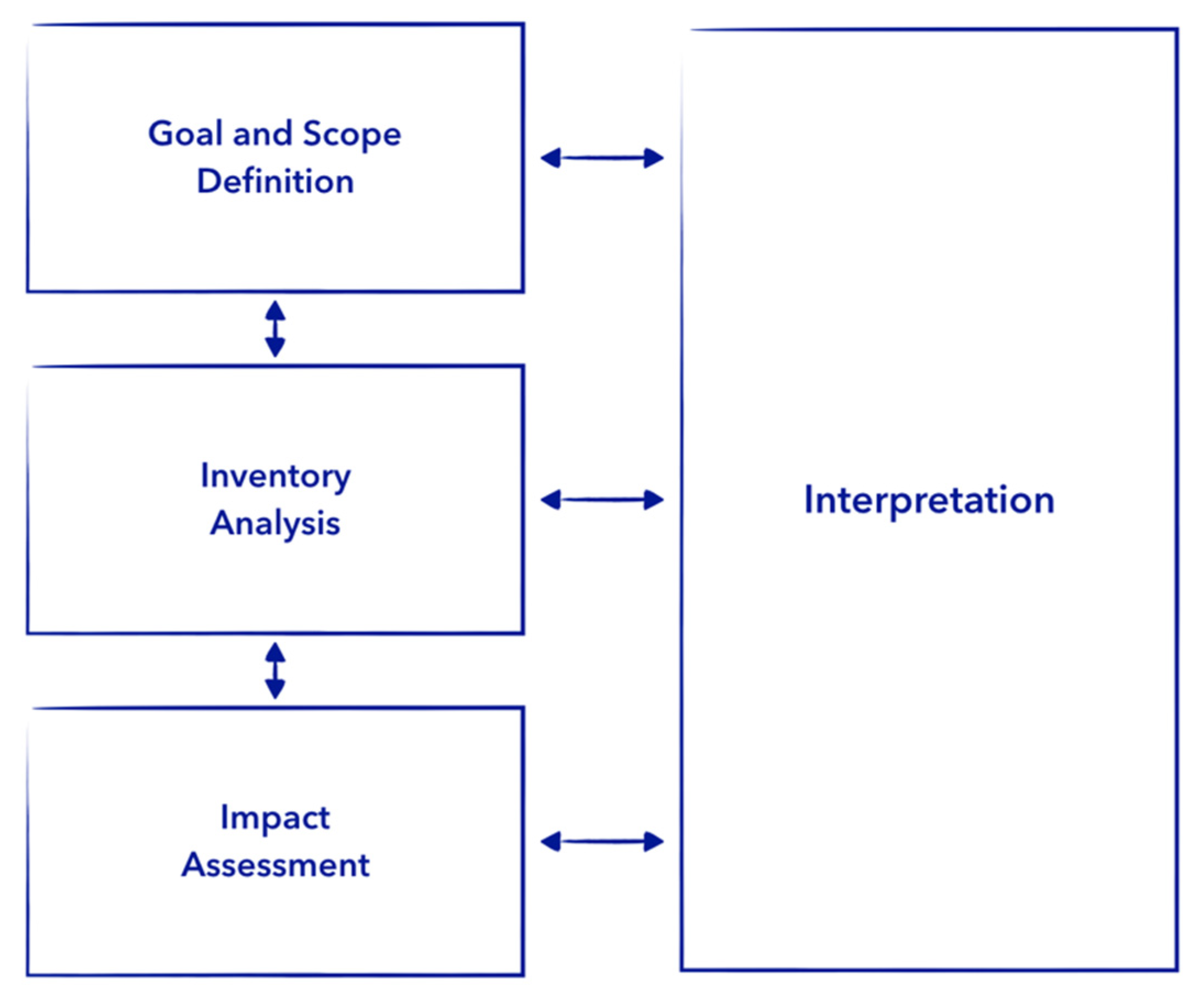
The ISO standardized framework comprises four compulsory phases—see Figure 1.

The first phase, Goal and Scope Definition, frames the study: The goal includes the reason for carrying out the study (why the study is done), its intended application (what the study wants to achieve), the intended audience and the commissioner of the study, and other stakeholders to highlight conflicts of interest. The scope, on the other hand, defines the functional unit and establishes the focus of the study in terms of the processes to be included in the product system (system boundaries). The functional unit represents a quantified function of the production system that is analyzed and essentially serves as the basis of the assessment.

Following the first phase, Inventory Analysis collects information about the physical flows in terms of input of resources, materials, semi-products, products, and by-products and the output in terms of emissions, waste, and the final product. It must be noted that that the validity and accuracy of LCA results are strongly dependent on that of the underlying inventory; for this reason, having access to high-quality data, e.g., collected on-site or extrapolated from design flowsheet, is of utmost importance.

Taking the life cycle inventory as a starting point, Impact Assessment “translates” the physical flows of the product system into potential impacts on the environment and human populations using knowledge and models from environmental and medical science. Impacts are expressed as their contributions to a set of pre-defined impact categories, each addressing a specific issue; for instance, the climate change category includes all gases contributing to the greenhouse effect. Finally, in the Interpretation phase, the results of the study are checked for consistency and completeness, and conclusions and recommendations based on the results of earlier phases are developed.

2.2. Multi-Risk Assessment

Risk assessment is commonly defined as the scientific process in which the risks posed by inherent hazards involved in the process or situations are estimated either quantitatively or qualitatively [6,7]. Therefore, to understand multi-risk assessment, one needs to have a clear the distinction between hazard and risk. In general terms, hazard is defined as the potential to cause harm, whereas risk is commonly defined as the combination of the probability, or frequency, of occurrence of a defined hazard and the magnitude of the consequences of the occurrence.

Historically, the introduction of risk assessment as a quantitative tool can be traced back to the 1950s and in the last 70 years, it has been used to support decision-making in both commercial and governmental organizations. Emerging with the goal to address concerns for human health, it has now evolved to include more general environmental concerns, and a number of different subdivisions within risk assessment have been developed.

In this article, we focus on multi-risk assessment, whose main goal is to harmonize the result obtained for different risk sources while also taking into account possible risk interactions [15,16]. An MRA may take into account both events threatening the same elements at risk without chronological coincidence—“Multi-Hazard assessment”—and/or related events (depending one to another or caused by the same triggering event), thus occurring at the same time or shortly following each other—“multi-risk assessment”—(European Commission 2010). In other words, such analysis is useful both to assess different (independent) hazards threatening a common set of exposed elements and to identify and assess possible interactions and/or cascade effects among different possible hazardous events [15,17,18,19].

The implementation of an MRA analysis needs:

To take into account the possibility of multiple (natural and anthropogenic) hazards as possible triggering mechanisms;
To explore all the plausible scenarios of cascading events, identifying the logical relationships among the different events driving to an unwanted consequence;
To assess the possibility of impacting different typologies of environmental and anthropic exposed elements.
Going into more detail, a quantitative risk analysis can be structured in three main steps [20,21]:
Identification and description of potential accidental events in the system (accidental event: A significant deviation from normal operating conditions that may lead to unwanted consequence);
Identification in a hierarchical structure—fault tree—of the potential causes of each incidental event using causal analysis (if probability estimates are available (of the basic events), these may be input to the fault tree and the probability/frequency of the accidental event may be calculated);
Identification in a hierarchical structure—Event Tree—of the potential consequences of each incidental event using causal analysis.

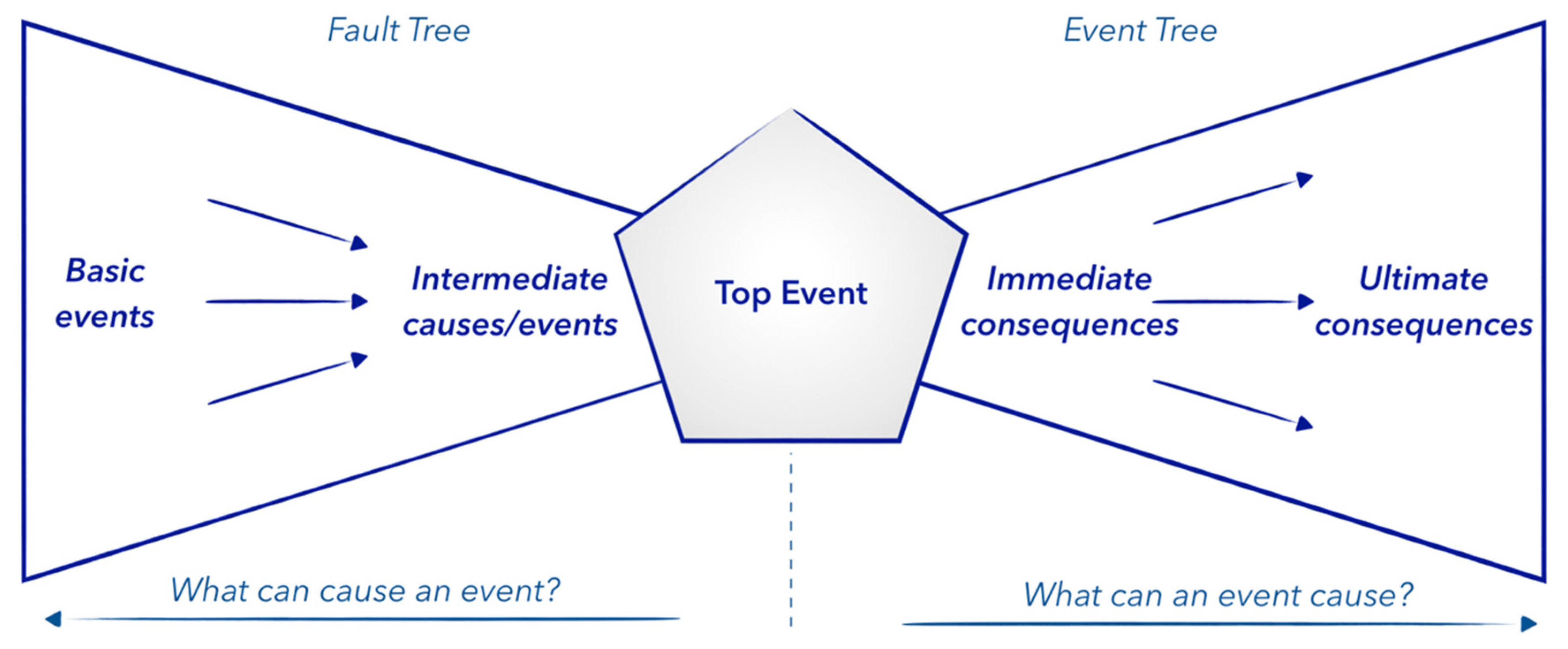
In particular, the general framework for the quantitative multi-risk analysis is exemplified using a so-called bow-tie structure—Figure 2. It is constituted of a fault tree on the left-hand side of the graphic plot, identifying the possible events causing the critical (or top) event, and an event tree on the right-hand side displaying the possible consequences of the critical event. Such a structure considers the possibility of multiple (natural and anthropogenic) hazards as possible triggering mechanisms, explores the logical relationships among the different events resulting in unwanted consequences, and assesses the possibility of impacting diverse kinds of environmental and manmade exposed elements.

The protocol is, thus, based on two analytical approaches: Probability theory and methods for identifying causal links between unfortunate effects and different types of hazardous activities.

2.3. Comparing LCA and MRA

The present literature on either LCA or (M)RA (here, the brackets indicate that the following is valid for RA in general and, as a consequence, also for MRA) studies of different geo-resource exploitation is rich, providing the scientific and industrial community with a better comprehension of the environmental impacts and the risks of individual geo-resources exploration and exploitation activities. Nonetheless, the two approaches are still used in a disjointed way; very few attempts have been done to consider both approaches in a single framework. Liu and Ramirez [12], in particular, presented a review of both LCA and RA methods, focusing their discussion mostly on a comparative analysis including the environmental consequences of both operational activities and failures, which helps in identifying the focuses, overlaps, and potential knowledge gaps of current research, but a proposal on how to integrate the two different approach is still missing in the literature of geo-resource exploration and exploitation.

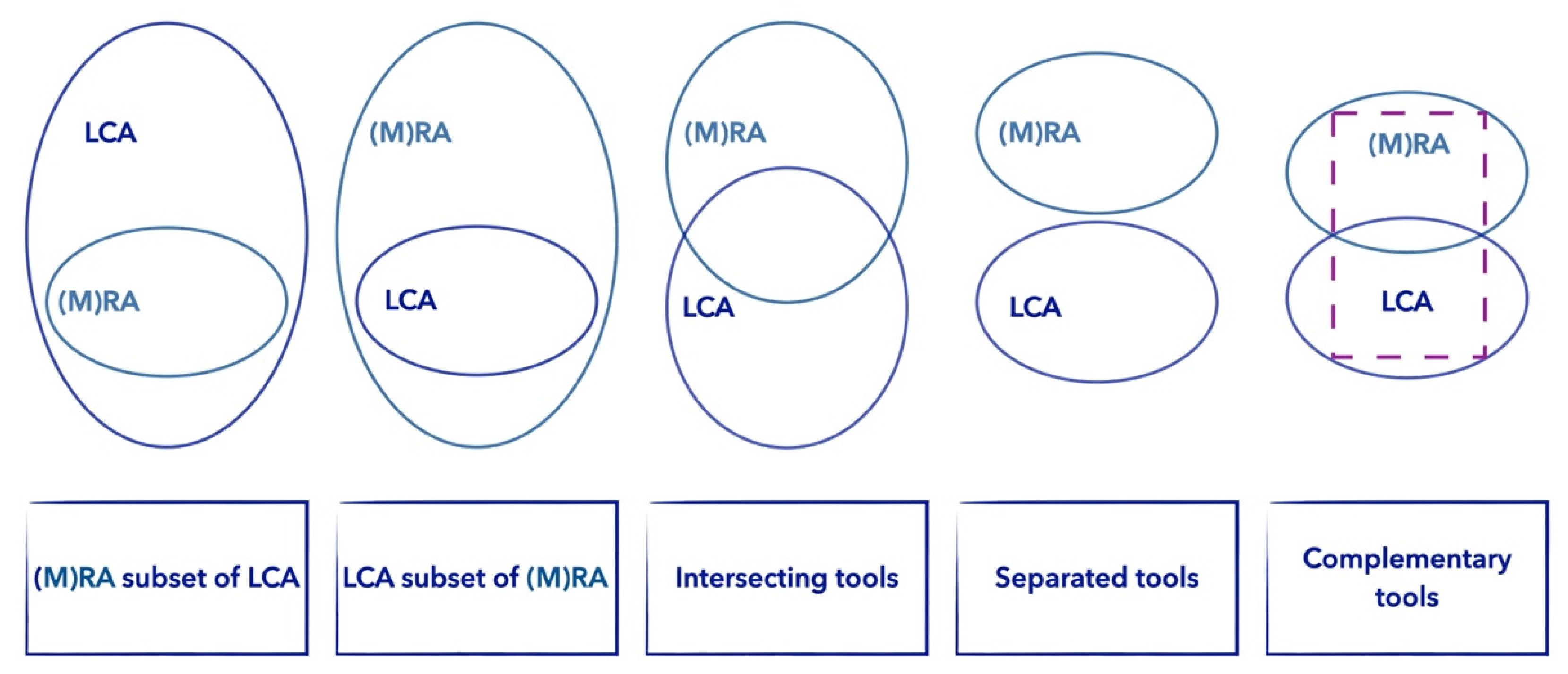
However, the applications of LCA and (M)RA in different industrial fields, e.g., pharmaceutical and chemical manufacturing industries, provide a potential way forward, as shown for example in Ref. [19]. It is important to note that some features of the two analyses depend on the field of application; nevertheless, the general approach still holds. In agreement with Ref. [13] suggestions, there are five different approaches in the comparison of LCA and (M)RA—Figure 3:

(M)RA can be considered as a subset to LCA;
LCA can be considered as a subset to (M)RA;
(M)RA and LCA can be considered as intersecting or overlapping tools;
(M)RA and LCA can be considered as separate tools;
(M)RA and LCA can be considered as complementary tools, each one with a particular perspective, both needed to get the full particulars.

To devise a more general protocol that integrates both approaches (i.e., MRA and LCA), it is useful to compare their specific features.

Both approaches encompass potential or probability of effects, even though one—LCA—deals with impacts caused by ordinary routine operations, and the other one—MRA—focuses on impacts caused by incidents due to system failures or extreme events. Such difference translates into the fact that MRA and LCA address distinct and different questions.

The similarities, differences, and interfaces between these two methods are more complicated questions than what may intuitively be apprehended [9,10]. In general, one may find many specific features that one analysis presents while the other does not. Nonetheless, it is possible to summarize all the differences in few main aspects:

Functional vs. actual units: A fundamental difference between LCA and MRA is that the former uses a functional unit, whilst the basis of the assessment of the latter represents the actual size or throughput of a plant. For example, the typical functional unit used in LCA studies for power generation technologies (including geothermal power plant) corresponds to 1 kWh (or 1 MJ) of electricity generated; whilst the actual unit considered in an MRA study may correspond e.g., to the installed capacity of the plant or to the amount of electricity generated in 1 year.
Global vs. local: A typical LCA spans the whole globe; this requires the use of location-independent impact assessment models to avoid making the analysis excessively complicated. An MRA analysis is strictly specific to one project, using site-specific information and data to estimate the environmental impacts. Moreover, LCA is time-independent, whilst MRA is not.
Deterministic vs. probabilistic impacts: Both methods adopt a life cycle perspective, but with a caveat. In fact, the definition of the life cycle of a project differs in the two tools: In the LCA, the life cycle of the project starts with the raw materials and ends with the closing of a site; RA analysis, on the other hand, includes the site abandonment and post-abandonment phase. Such a difference is motivated by the fact that, while LCA is focusing on the deterministic impacts of the project, which are null once the site has been abandoned, MRA addresses the impacts of the probable accidents, which can happen also after the closure of the site.
Receptor vs. loading: One of the main goals of an MRA is to predict the possible environmental impacts of a project—receptor focused—while LCA aims at reducing the overall pressure on the environment of an entire project system from cradle to grave—loading focused.

3. MRA and LCA: An Integrated Approach

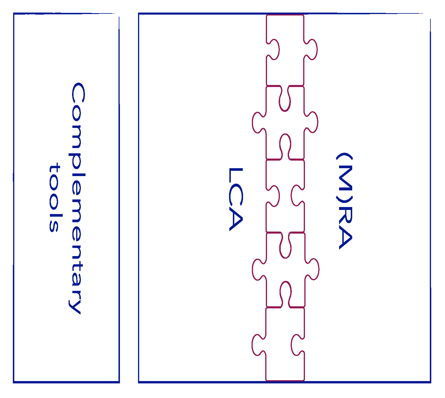
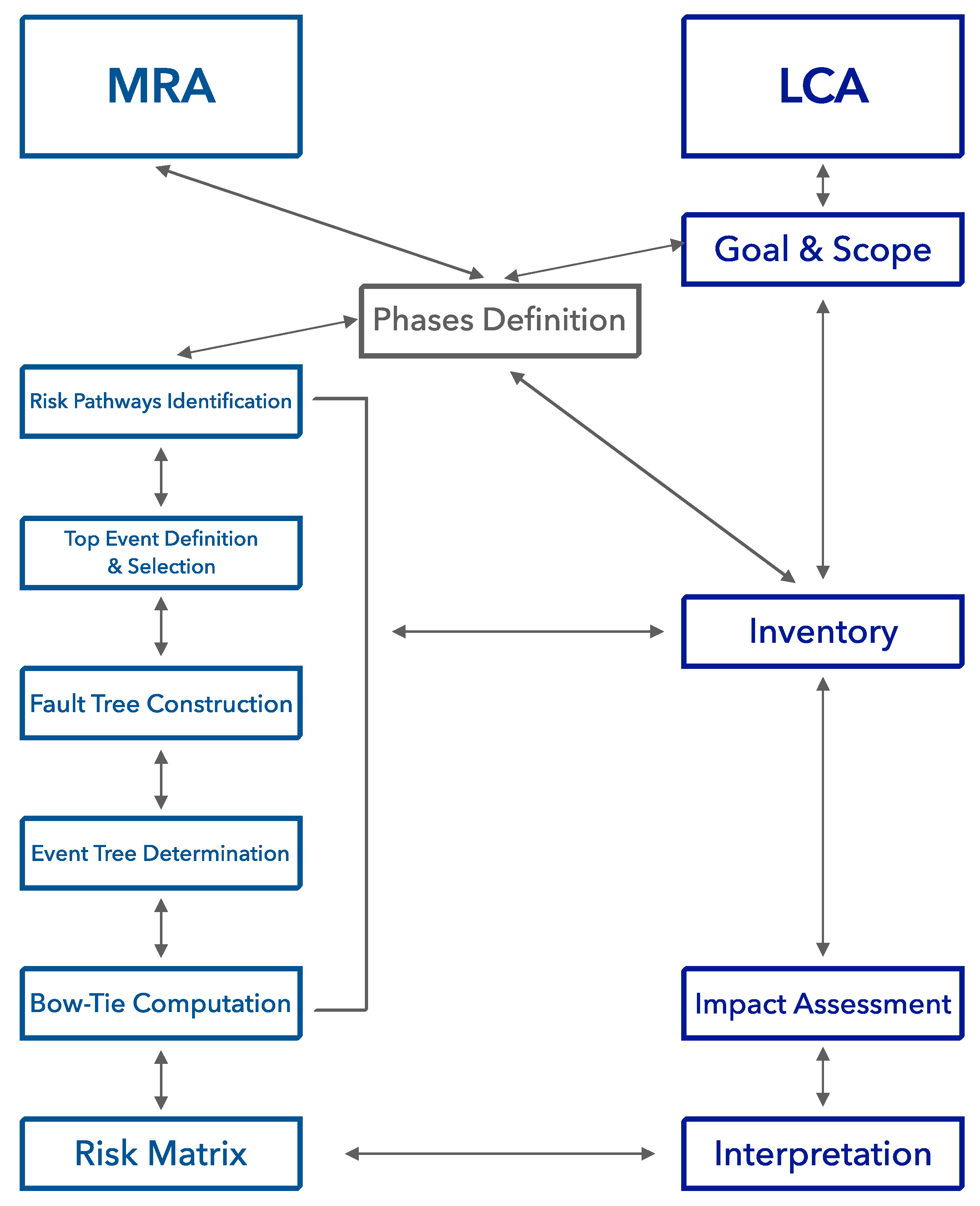
As noted in Section 2.3, there are fundamental differences between LCA and MRA and therefore a full integration may not be possible. Nonetheless, we believe that these two tools can be applied in complementary manner as two parts of a comprehensive framework to evaluate certain and potential impacts—Figure 4.

More specifically, MRA can be built upon LCA both qualitatively and quantitatively. In fact, one may use the LCA approach and results to identify and address the possible risk pathways. On the other hand, the outputs of the Life Cycle Inventory can be used to define operational parameters of the probabilistic framework of the multi-risk assessment. We note that, although the implementation of this approach may vary depending on the different field of application, the approach itself is quite general and still holds in the other industrial cases, where it is also much needed, (e.g., [11]).

In the next sections, we present a protocol to integrate LCA and MRA in a specific case study on geo-resources’ exploration and exploitation.

Geo-Resources Exploration and Exploitation

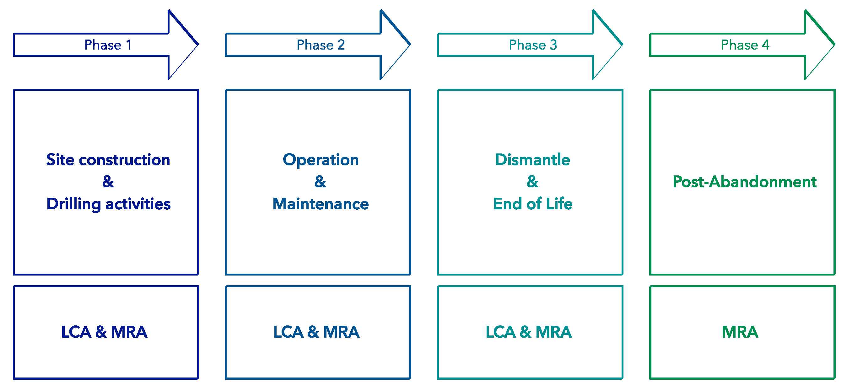
Once a given project has been chosen, the first step in harmonizing the two analyses is to divide the project life into the same phases, e.g., site construction and drilling, operation and maintenance, dismantle and end of life, and adding the post-abandonment phase for the MRA only, see Figure 5. Such a measure will allow the best use of the LCA inventory to set some of the input data of the MRA.

The LCA inventory provides, in fact, crucial knowledge on the amount of hazardous material on-site related to the functional unit, thus allowing to better identify the possible hazard sources for which it will be necessary to estimate probabilities and intensities of related hazards through MRA.

Moreover, LCA results may highlight specific risk pathways that lead to the possibility of confronting routine impacts and risk impacts for specific elements of the project with important insight for the risk and impact mitigation.

On the other hand, MRA results may be interpreted as an additional error on the impacts computed by LCA, producing results regarding additional possible impacts weighted by their probability occurrence.

A schematic of the protocol is in Figure 6. From an environmental point of view, the key outcome of this combined approach is the possibility to evaluate impacts of a given geo-resource development project from two perspectives: On the one hand, LCA will produce assessments that can be interpreted as expected (a relatively certain or ‘very likely’) impacts mostly caused by the normal (routine) development of the project. On the other hand, MRA will produce assessments of likely impacts caused by the random occurrence of extreme events (e.g., system failures, as well as the effects of natural or anthropic events), each of which is weighted by their probability of occurrence. The integrated analysis of such “certain” and “probable” impacts may provide important clues for a comprehensive evaluation of the potential impacts associated with a given project, which in turn may provide objective quantitative information for sound cost/benefit analyses. Such an approach can also open new perspectives in harmonizing deterministic and stochastic impacts. In fact, using the LCA outputs as inputs of the MRA can allow the analyst to focus on particular risk pathways that could otherwise seem less relevant but can open new angles in the risk/impact evaluation of single elements.

To demonstrate the performance of this kind of implementation, in the following, we will take into consideration a virtual case tailored to represent a real geothermal power plant, implement our approach on it, and present the results of such analysis.

4. Presentation of the Case Study

Our case study is a virtual site tailored to represent a real one, with data elements from both the real and the fictitious site. The real site is United Downs Deep Geothermal Power Project (UDDGPP) in Cornwall, a geothermal binary power plant that exploits the presence of a fault zone. Ref. [22] In particular, the project establishes circulation over a large vertical distance through the natural fracture system within the Porthtowan Fault Zone, by the use of a downhole pump and two deep, deviated wells. According to the value of the permeability, the large well separation (2000 m) enables flow rate and heat transfer area for commercial energy extraction. Thus, two deep, directional wells have successfully been drilled; the production well to a depth of 5275 m and the injection well to 2393 m. Both wells have intersected the target Porthtowan Fault Zone located approximately 800 m to the west of the site. The project aims to produce water to surface at a target temperature of 175 °C and circulate it in a binary cycle power plant to produce at least 1 MW of electricity. The maximum capacity of the power plant is limited to 3 MW by the existing connection to the grid [23,24].

The choice of applying the analysis to a virtual site has the advantage to obtain more general conclusions without invalidating the integration protocol. In fact, LCA is a general analysis that focuses on the type of production system and not on the site-specific features, which are investigated in the MRA. UDDGPP presented two key features that directed our choice: On the one hand, it was being built in parallel with our analysis granting us the possibility of live data, whilst on the other hand, the LCA analysis was already available [23,24] making it easier to focalize on the LCA-MRA integration problem, the main research question guiding this paper, and on the derived MRA.

We therefore focus on key risk pathways scenarios from upstream activities in geothermal energy production systems to assess impacts on primary risk receptors, such as the pollution of surface—or ground—water resources.

4.1. LCA

Paulillo et al. [23,24] performed a comprehensive prospective attributional LCA study on UDDGP; the study was aimed at assessing the future potential environmental impacts of the plant when operational (prospective perspective), without considering the possible consequences of choices made based on the results of the study (attributional approach). The study adopted a complete, cradle-to-grave system boundary that included the three typical phases of construction and drilling, operation and maintenance, dismantle, and end of life. The life-cycle inventory was based on site-specific data, primarily describing the construction of the wells, and literature data, for example from the Hellisheidi geothermal plant in Iceland [25]; the key inventory parameters are reported in Table 1.

The analysis was performed in Gabi (an LCA software) using the EcoInvent database, version 3.5 [26]. The full inventory, as well as numerical values for the LCA results, are reported in [24].

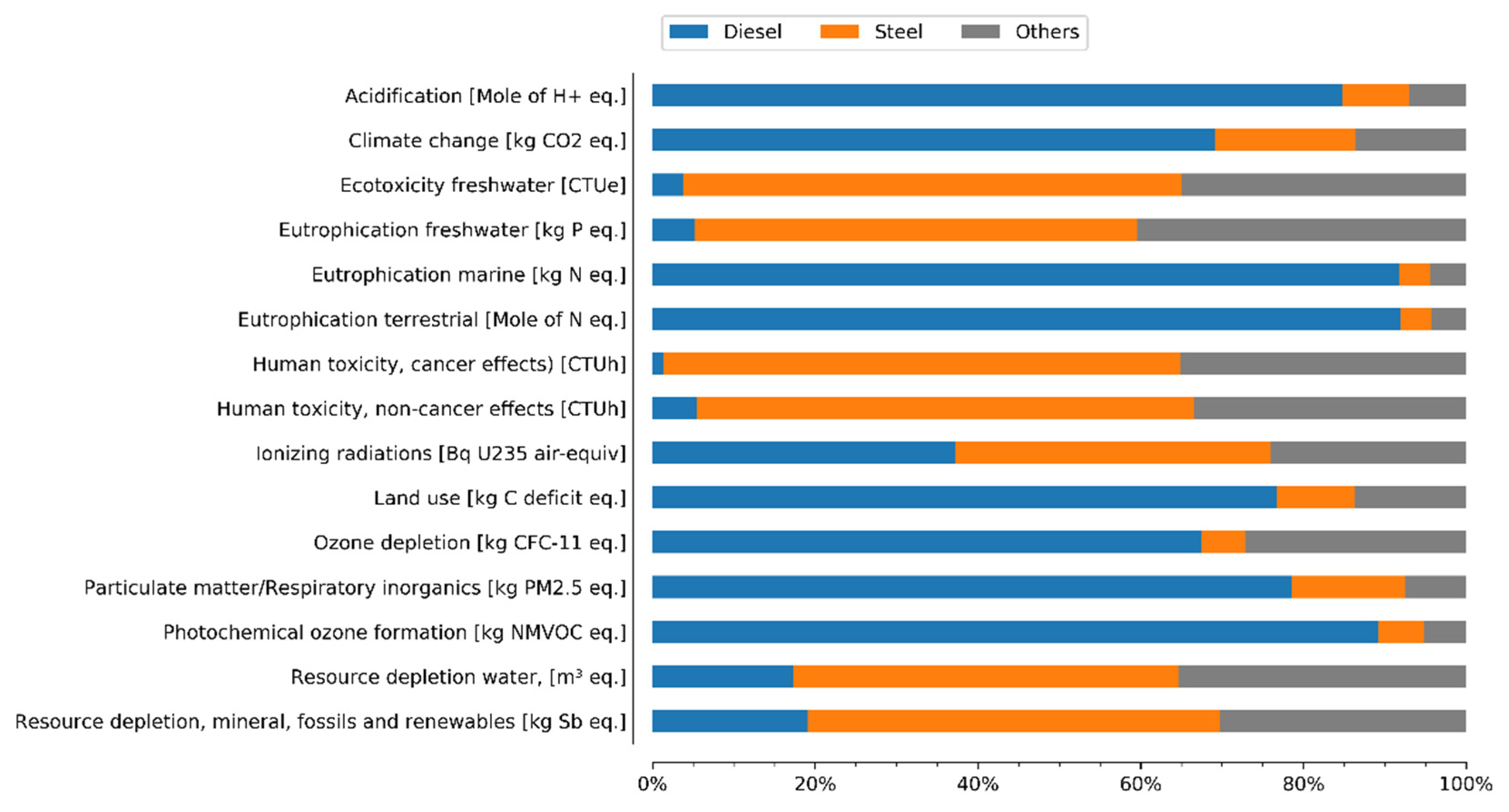
The study had three objectives: (i) Identifying the largest sources of environmental impacts, (ii) investigating the effects of several projects’ variables (e.g., the installed capacity of the power plant, or the requirement for stimulating the geothermal reservoir), and (iii) comparing the environmental performance of the UDDGP plant (and, by extension, that of the putative geothermal energy production in the UK) with other key energy sources in the UK. The hot-spot analysis showed that the vast majority of the environmental impacts originate from the construction phase, in particular from the use of diesel oil for powering the drilling rig, and of steel as casing for the geothermal wells—see Figure 7.

In light of these results, the authors argued that the most effective strategy to improve the environmental performance of UDDGP is to increase the lifetime of the project, including that of the geothermal wells, the power plant, and also crucially that of the underlying geothermal reservoir; this would reduce the environmental impacts of the construction phase per unit of electricity generated. Other strategies proposed included reducing, where possible, steel and diesel oil consumption, or replacing them with environmentally advantageous alternatives. A notable example is the use of electricity instead of diesel oil during drilling, which has recently been implemented at Hellisheidi [25].

The scenario analysis demonstrated that increasing installed capacity from 1 MW to 3 MW and cogenerating heat and electricity represents the most optimistic scenarios for UDDGP; each of these scenarios entails a ~30% increase in the environmental performance compared to the baseline scenario. The comparative analysis showed that from a climate change perspective, electricity from geothermal energy in the UK is environmentally preferable to that generated from natural gas and also from utility-scale solar photovoltaic, whilst being competitive with that from nuclear-pressurized water reactors and offshore wind farms. Nevertheless, the environmental advantages of geothermal energy are not forthright when other environmental categories were taken into consideration; for example, geothermal energy had the highest environmental impacts in the category particulate matter formation.

4.2. MRA

For the MRA, a bow-tie structure [15,19,20] was used. It is composed of a fault tree on the left-hand side of the graphic plot, classifying the possible events causing the critical (or top) event, and an event tree on the right-hand side displaying the possible consequences of the critical event. Such a structure considers the possibility of multiple (natural and anthropogenic) hazards as possible triggering mechanisms, explores the logical connections among the different events resulting in unwanted consequences, and considers the possibility of impacting different typologies of environmental and manmade exposed elements.

4.2.1. Risk Pathways Identification

The implementation of a virtual site requires a clear definition of the phases that will be represented in the multi-hazard risk modelling process.

Thus, the first step we took, in order to harmonize MRA and LCA, is to divide the project life into the same phases used by LCA, i.e., site construction and drilling, operation and maintenance, dismantle, and end of life, and adding the post-abandonment phase, see Figure 5. Such measure allows the best use of the LCA inventory data.

As already mentioned before, the main risk pathway scenarios have been then identified for every phase of the project following the approach used by Garcia-Aristizabal et al. [15,19], which is structured into three main steps:

To consider the possibility of multiple (natural and anthropogenic) hazards as possible triggering mechanisms,
To investigate all the plausible scenarios of cascading events, detecting the logical relationships among the different events driving to an unwanted consequence,
To evaluate the possibility of impacting different typologies of environmental and anthropic exposed elements.

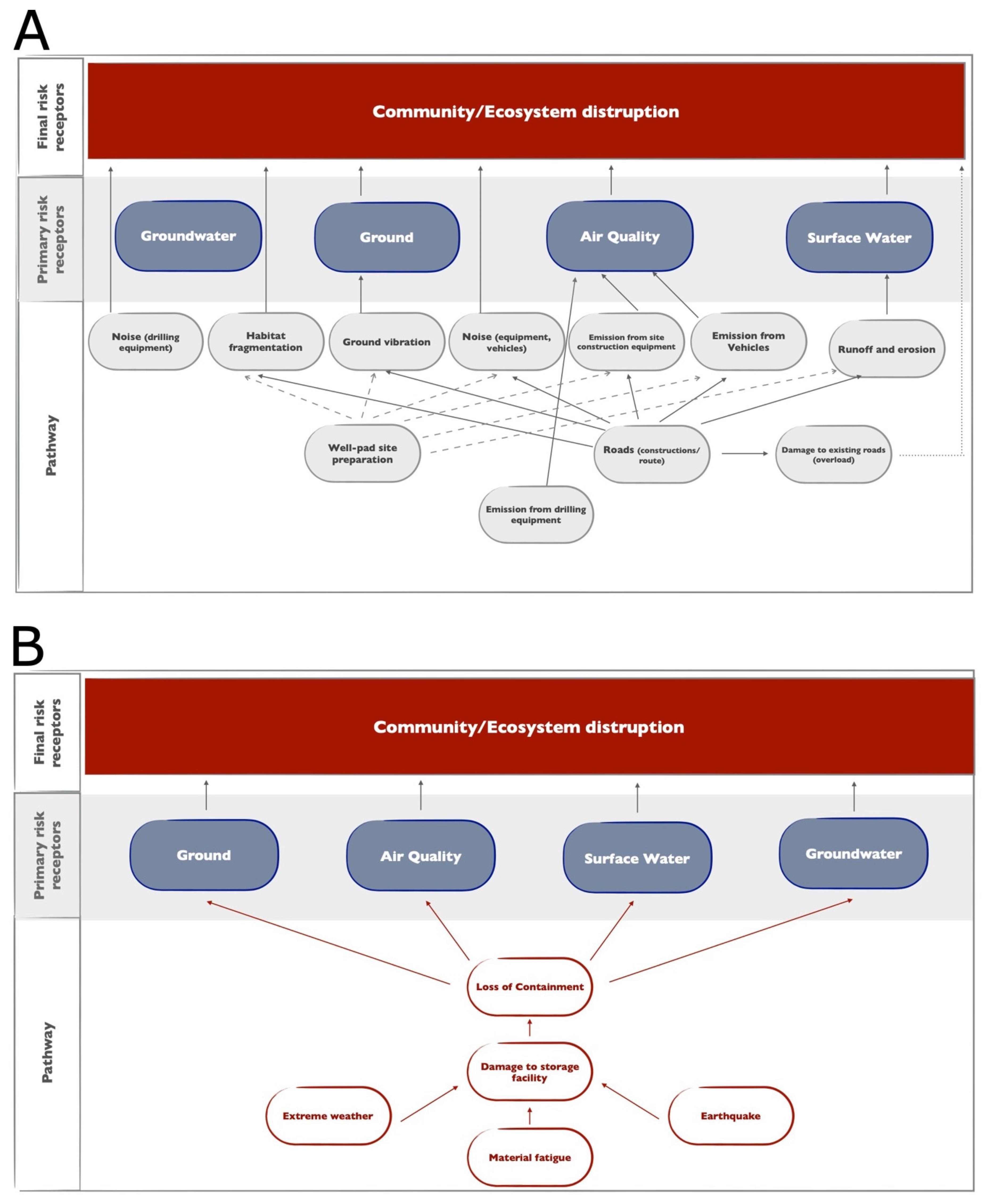
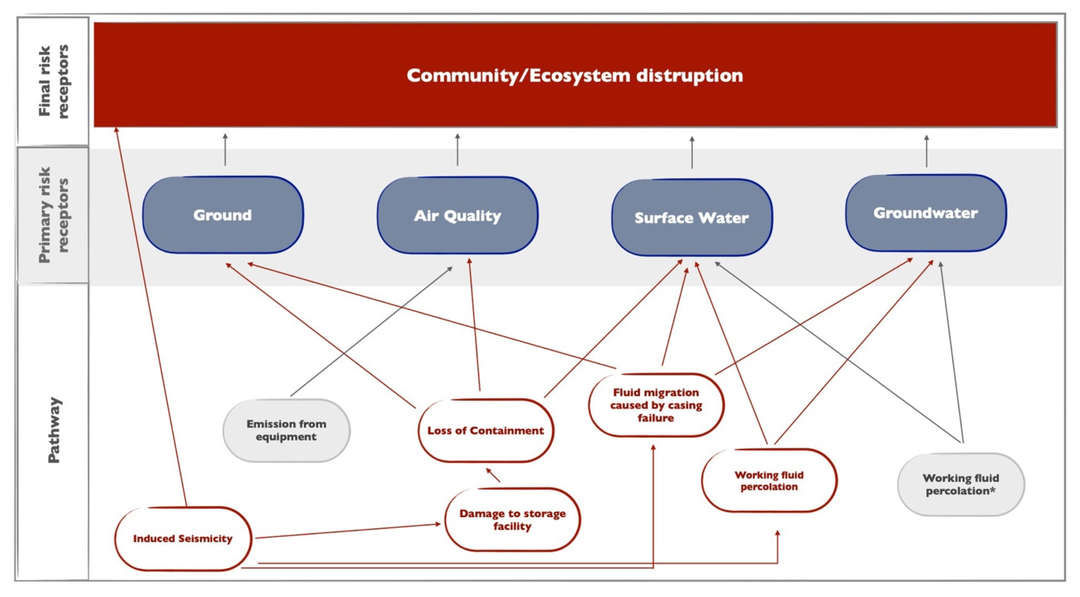
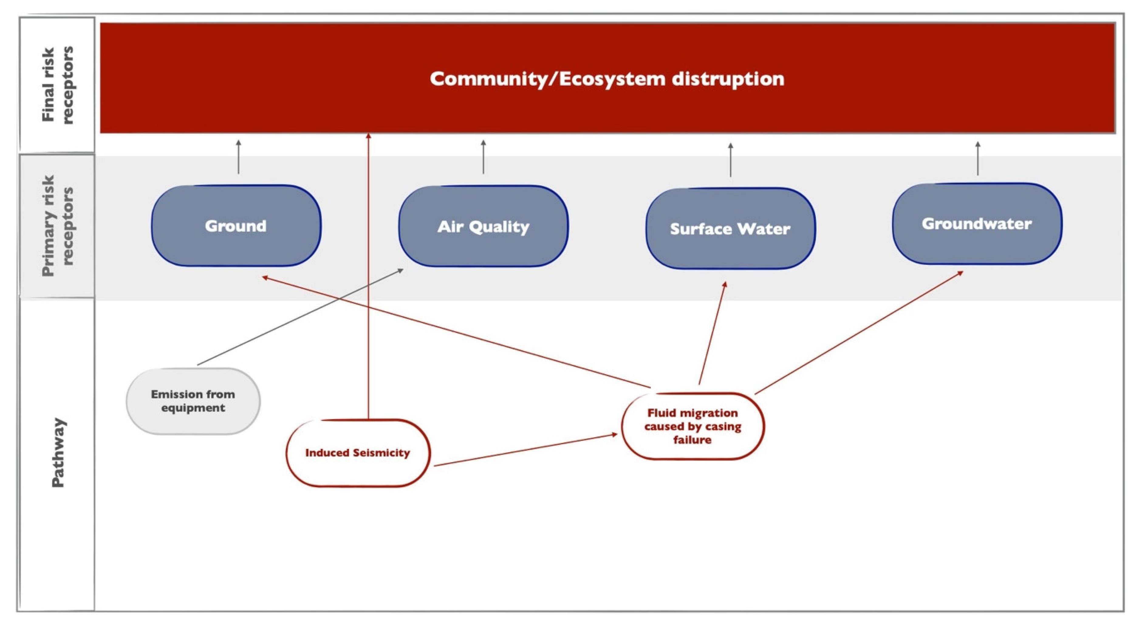
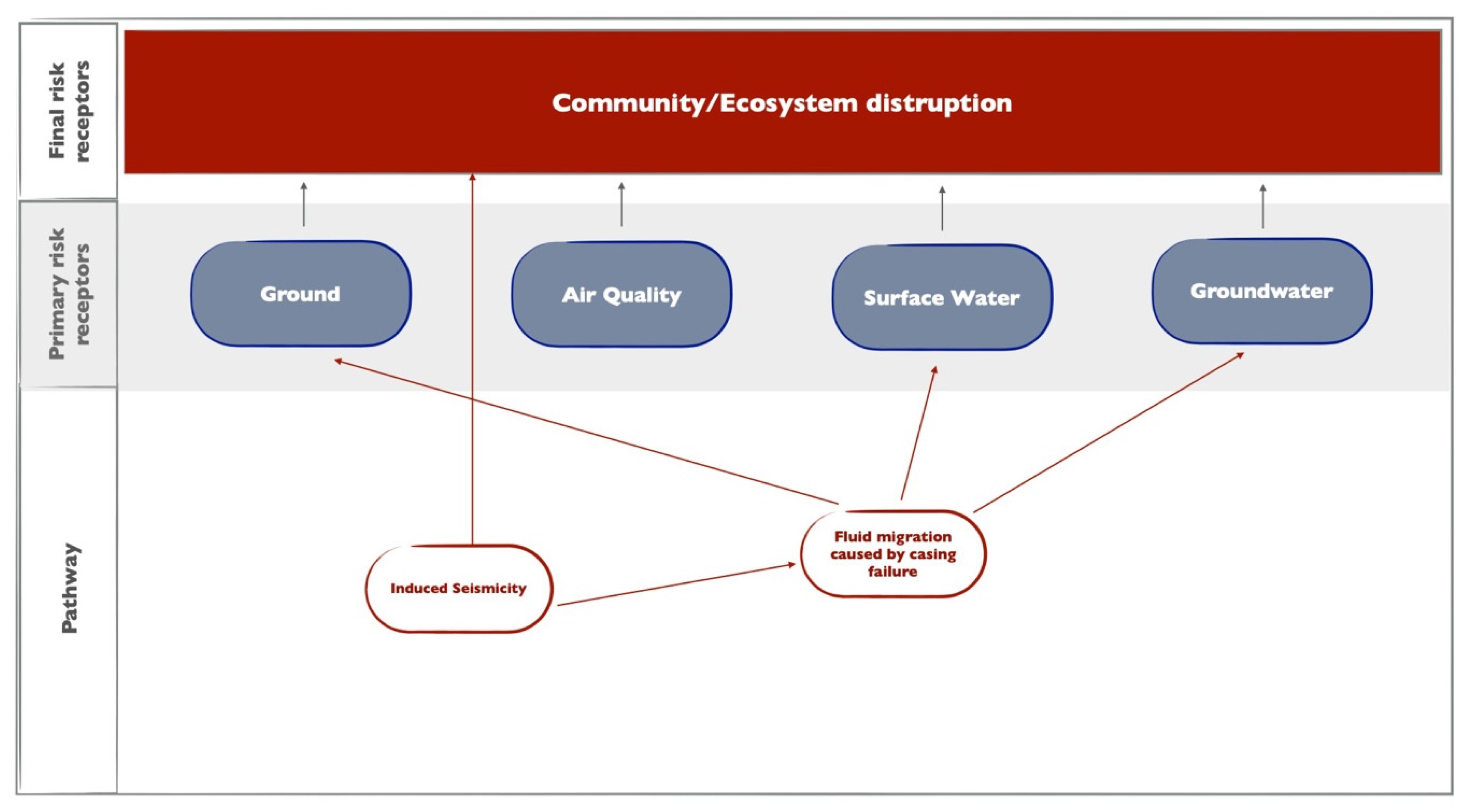
The main risk pathway scenarios, corresponding with environmental impacts associated with routine activities as well as with potential incidents and/or extreme events, have been identified in the causal diagram for each of the four phases of the project respectively in Figure 8, Figure 9, Figure 10 and Figure 11.

We want to stress here that when analysing the possible accidents, to identify and select the different risk pathways, it is important to define a criterion to prioritize them according to the relevance the risk pathway would pose in the overall analysis. This article aims to explain the methodology of the protocol developed and to show its application to a case study. The choice of using a virtual site based on UDDGPP as a case study was motivated by several characteristics, in particular: The existence of an in-depth LCA analysis, the installation on site of a dedicated seismic network that started recording data already in the drilling phase, and the possibility of following live all the phases since our analysis started with the project. At the same time, this last feature meant that the phases following construction and drilling have not yet been carried out and therefore the relative data with which to define the virtual site do not exist. For this reason, the analysis of the case study focuses on the first phase of the project: Construction and drilling. Within this same phase, the risk pathway that has been privileged is the one for which less use of elicitation should be made.

From such casual diagrams is possible to identify the main risk pathways: Phase 1—Risk related to Diesel Storage; Phase 2/4—Risk related to Induced Seismicity. However, for the purpose of this article, we focus on the former: Diesel Storage. This is in fact of particular interest considering that (i) routine impacts are specifically present in phases 1 and 2 of the project—i.e., site construction and drilling, and operational and maintenance—and (ii) the results of LCA show diesel oil as the main source of impact in the overall life of the project, thus indicating the related risk pathway as the principal one to test our approach.

4.2.2. Structuring Scenarios

Following the risk pathway already presented in Section 4.2.1, it is possible to define the risk pathways scenarios as shown in the graphs in Figure 8, which represent the fault trees of our Bow-tie approach.

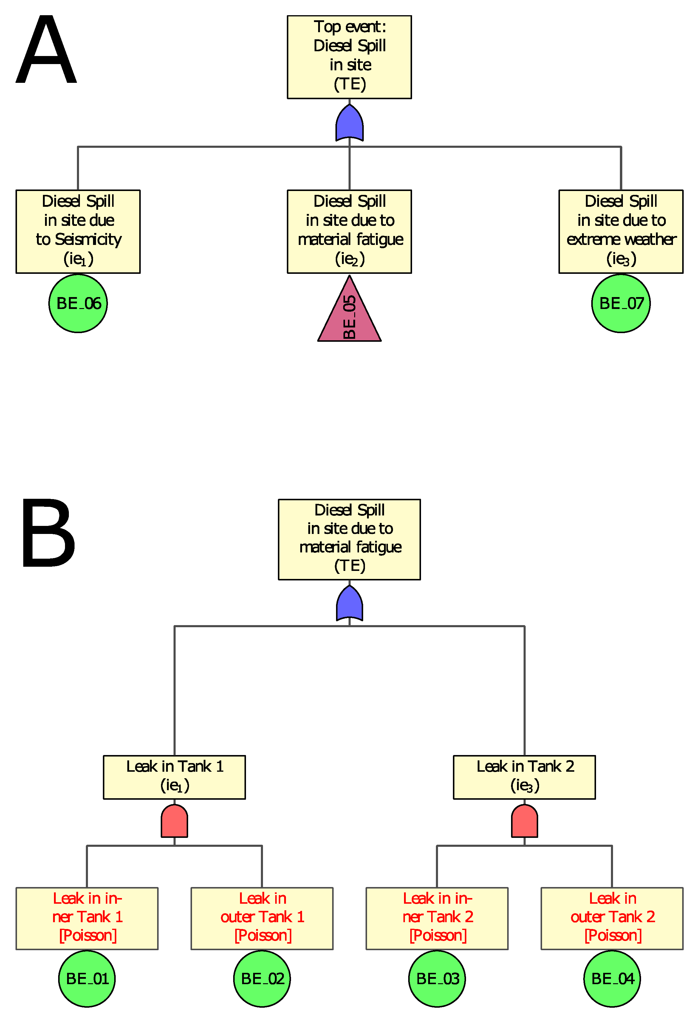
The risk pathway scenarios of this phase imply the definition of six basic events (BE_0n). In particular, Figure 12A shows the fault tree for the diesel oil spill on-site, displaying both the natural and the anthropogenic source of risk, Figure 12B shows the fault tree for the diesel oil spill on-site due to material fatigue, which is connected to Figure 12A through the connector represented by the red triangle. Table 2 summarize the description and the probabilistic models used for assessing basic event probabilities for this phase. Finally, the details regarding the probabilistic models used for setting the Bes probabilities (rates) are presented in Appendix A.

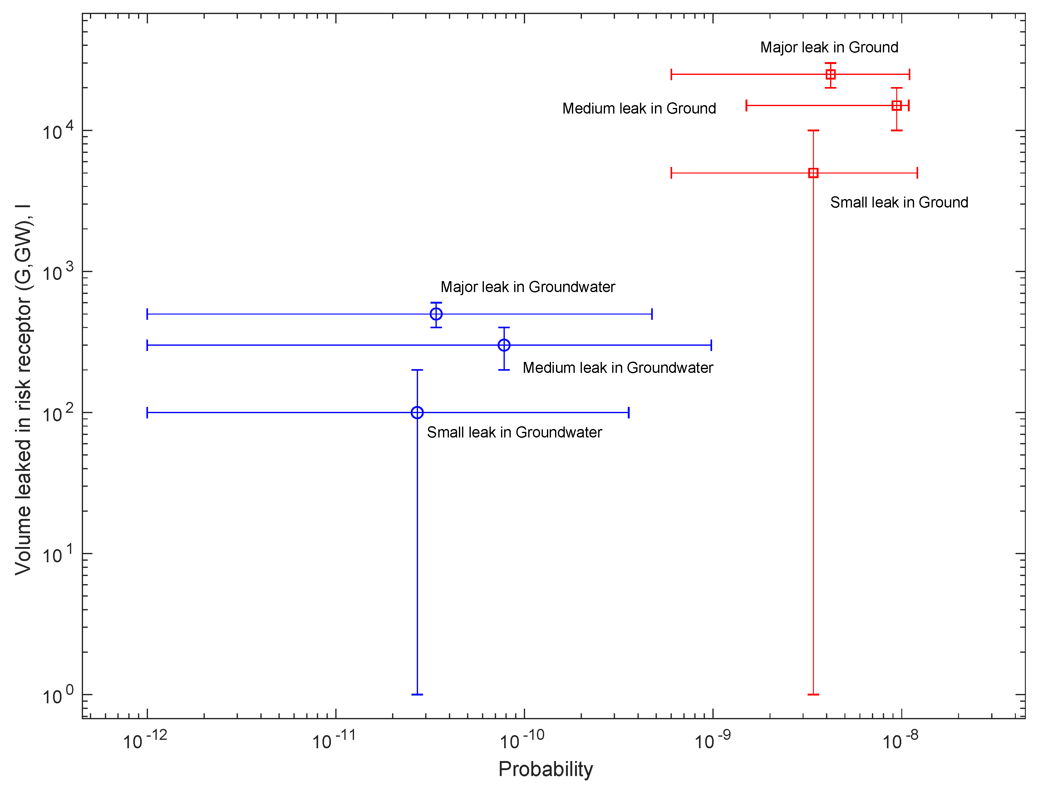
Starting from the T.E. of Fault Tree 1 it is possible to define two Event Trees, addressing its possible consequences for the risk primary receptors, respectively groundwater (Figure 13) and ground (Figure 14).

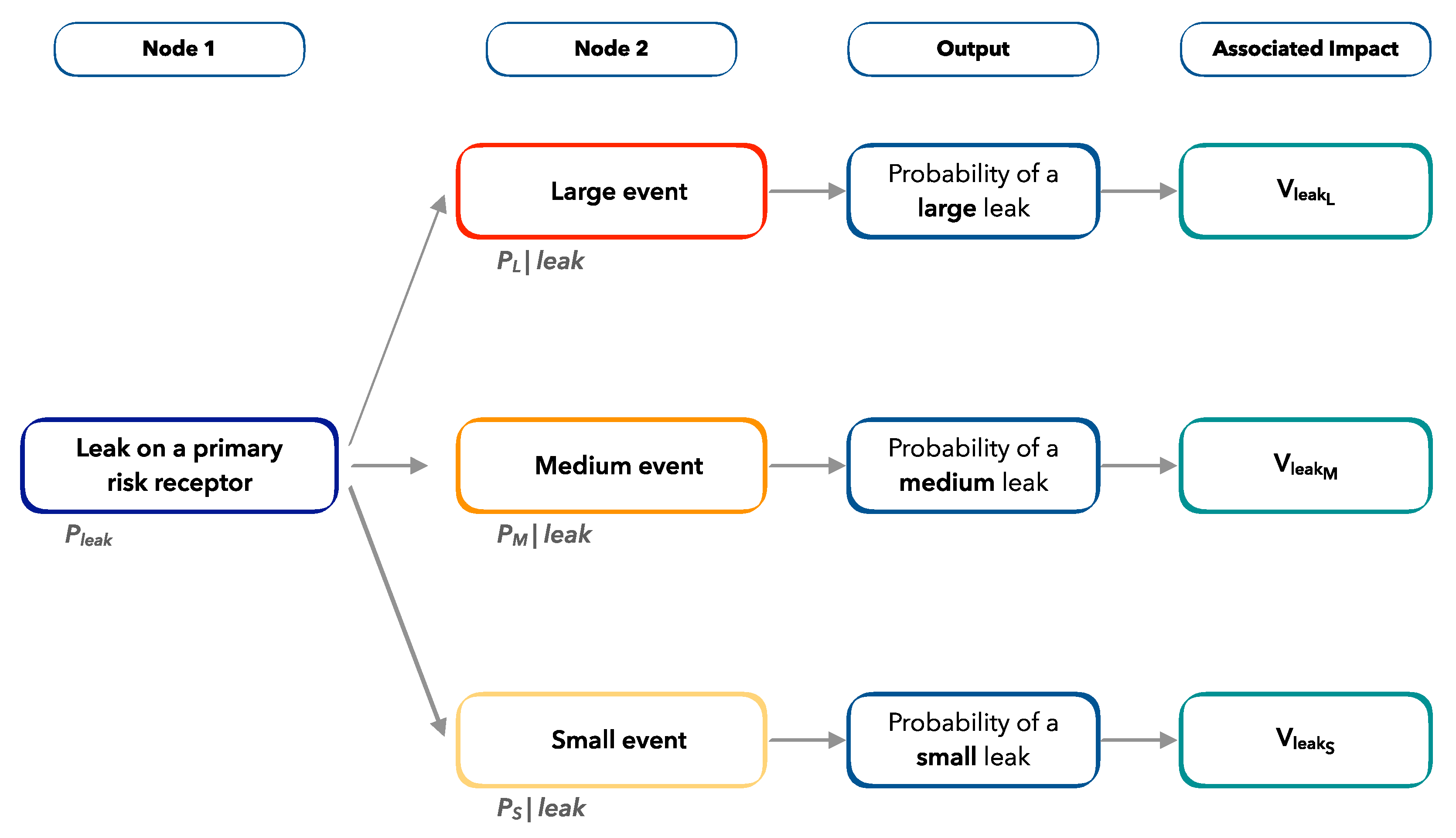
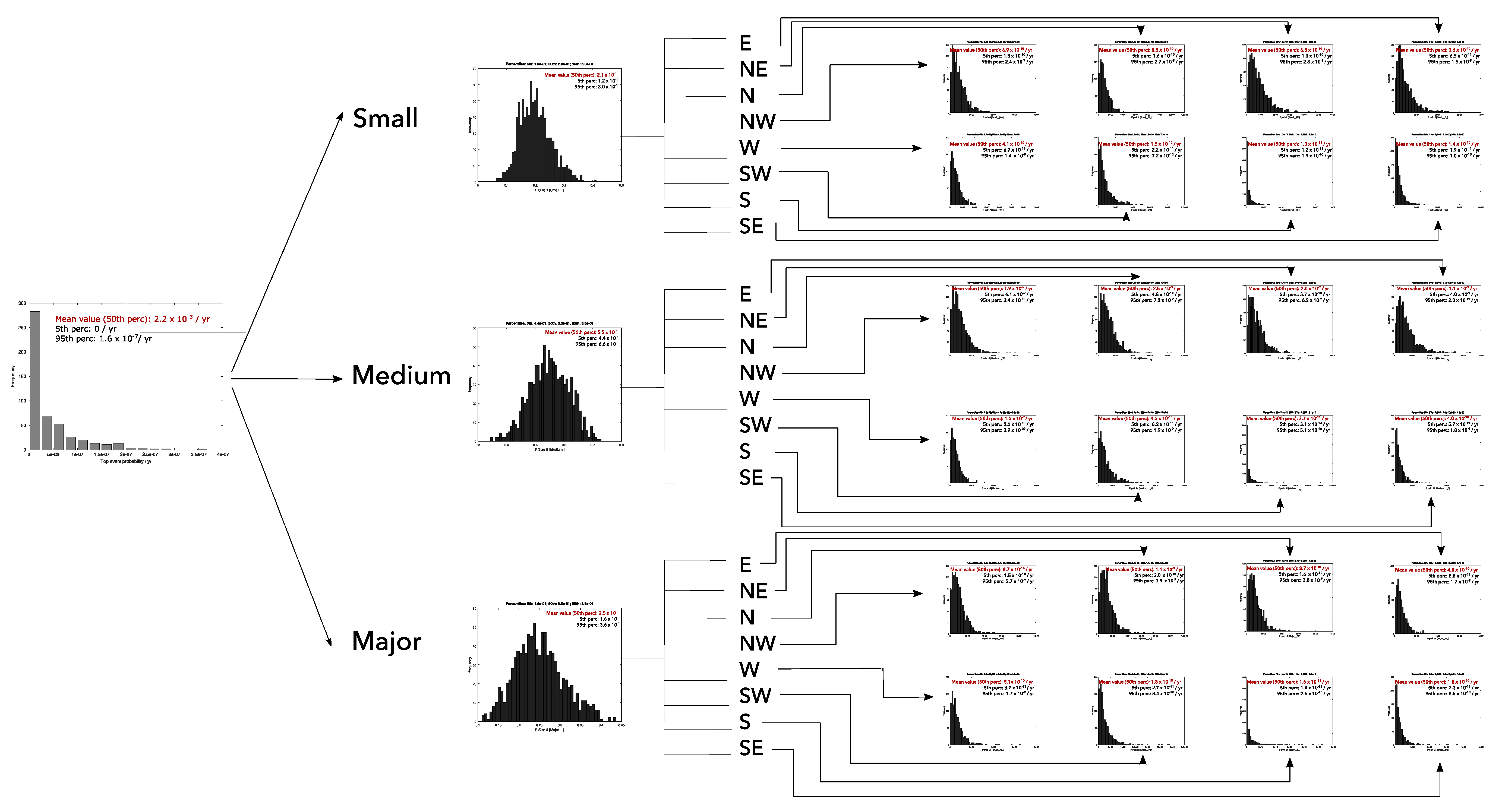
In fact, The general problem of the impact assessment, in this case, can be solved using a simple event-tree implementation that follows the structure depicted in Figure 13. Node 1 refers to the estimation of the leak probability, which is determined from the output of the fault tree analysis (e.g., the top event, or some intermediate event of interest). Node 2 refers to the “size distribution” of the event (here for simplicity divided only in three categories defined as “small”, “medium”, and “large”). These “size” events refer to the size of the typology of the event associated with the leak at Node 1. The combination of these two nodes provides the probability of each path of the event tree.

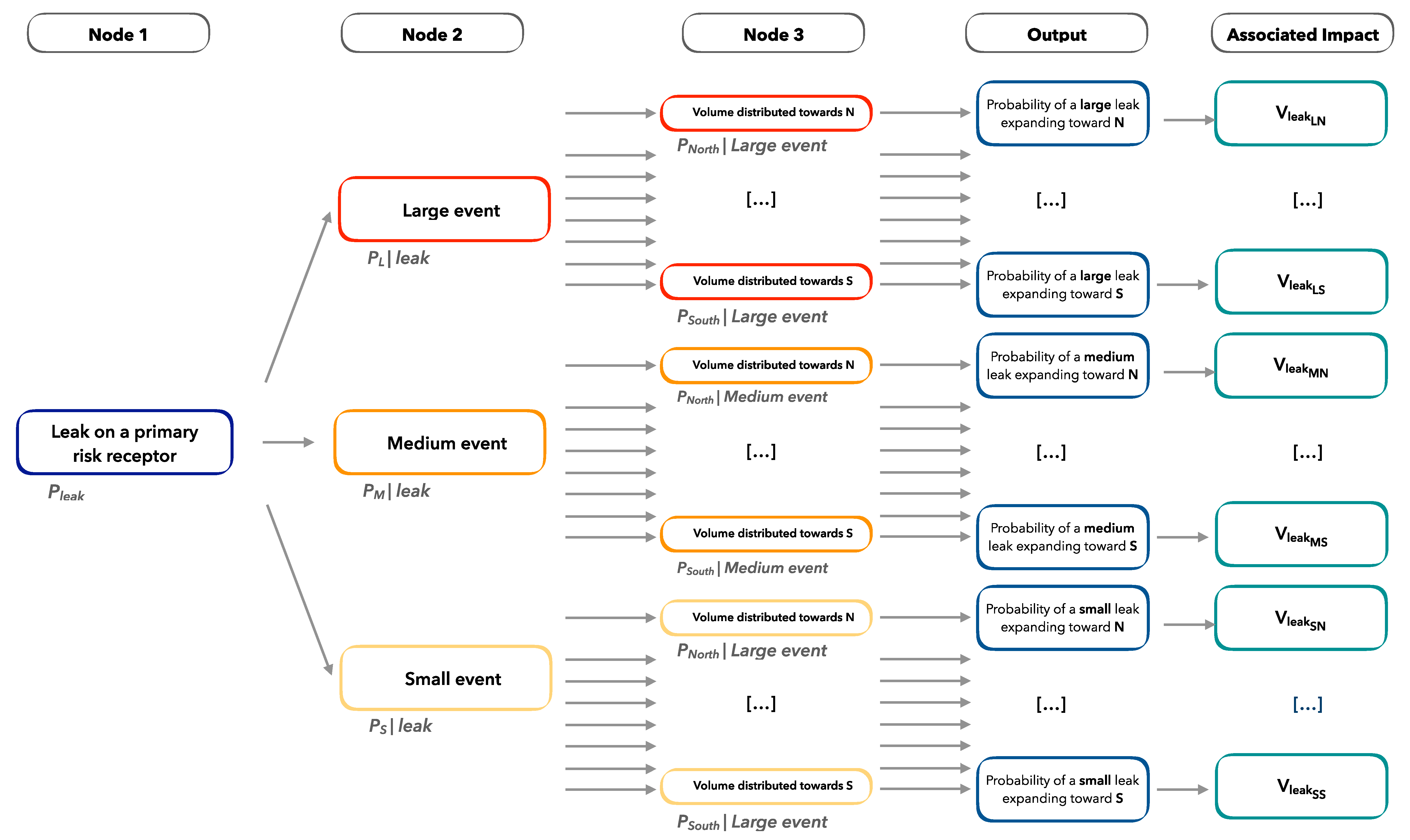
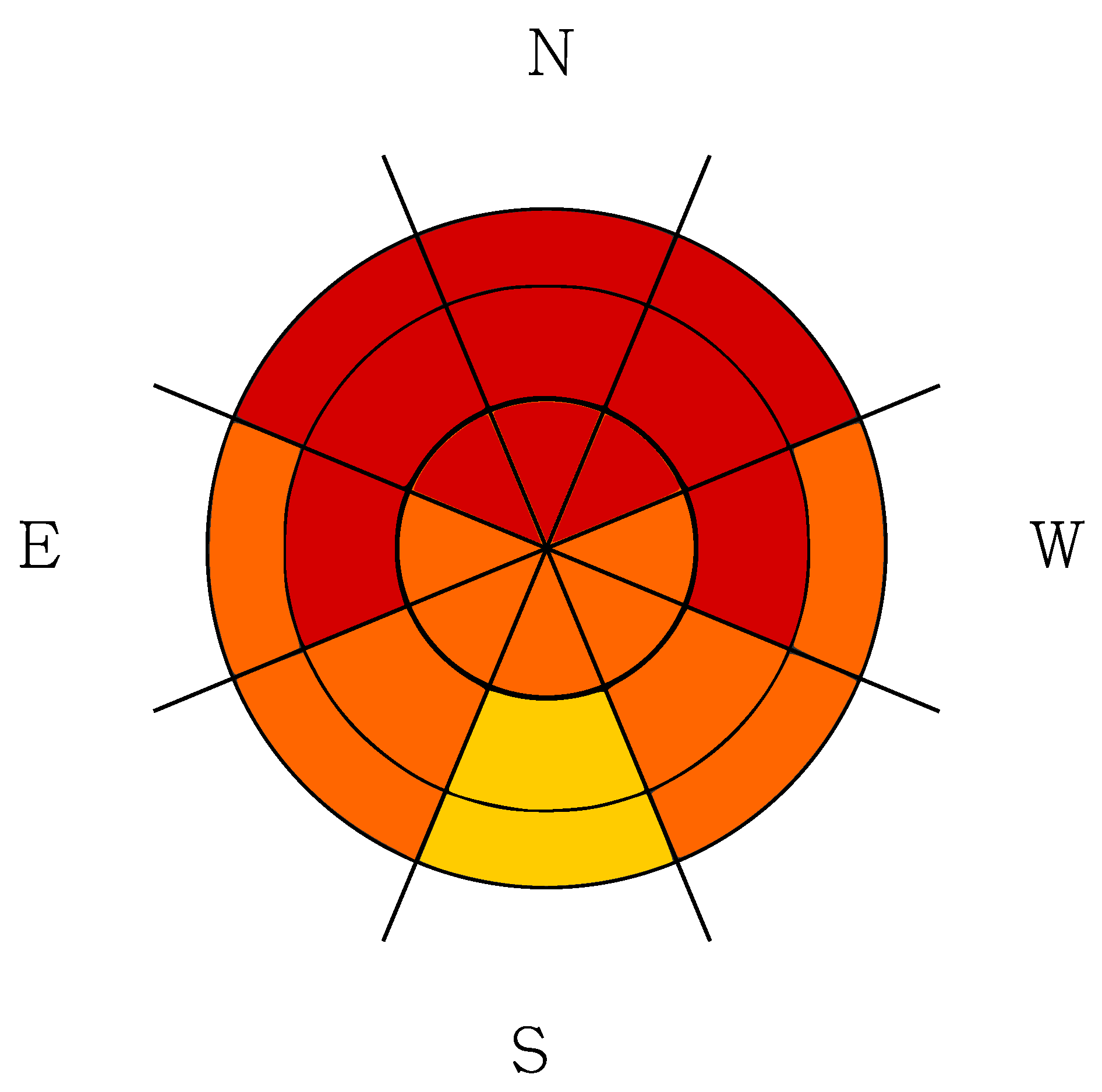
Moreover, the considered event tree can be expanded further considering different directions for the leakage spatial distribution, as shown in Figure 14.

5. Results and Discussion

5.1. MRA Results

In the following, we summarize the results obtained from the fault tree analysis and implement the event tree for performing impact assessment (considering the event “pollution” of the same risk receptors).

5.2. Probability of Impacting Primary Risk Receptors Considered

The first result obtained from the analysis is the probability of impacting the primary risk receptors we considered, evaluating the fault trees. In Figure 15, we find the histograms for the probability of, respectively, an oil spill due to material fatigue and an oil spill reaching the ground during the site construction and drilling phase. The mean values of the two distributions are of the same order of magnitude, i.e., 10⁻⁸.

5.3. Impact Assessment and Risk Matrices

Using the results obtained for the top event, we have thus implemented the structure of the two event trees to assess the impacts on the primary receptors of choice: Ground—Figure 14—and groundwater—Figure 13—under the elicited assumption that 2% of the volume leaked reaches the groundwater. After computing the expected leak volumes associated with each path of the event tree, impact assessment in this work is defined by taking into accpunt the expected leak volumes for different incidental events along with the respective occurrence probability. This information can be summarized using a classical risk matrix—Figure 16.

Moreover, considering the event tree in Figure 14, it is possible to define a spatial risk matrix. In fact, sampling the probability distributions defined at each node of the event ree and calculating the probability of occurrence for each path of the three, as shown in Figure 14, it is possible to plot the 50th percentile of the distributions for each distance and direction, obtaining a spatial risk matrix, as shown in Figure 17.

In particular, Figure 18 shows the sampling distribution at each node of the event tree in Figure 14. Starting from the top event we can see (in grey) its probability distribution. The first node differentiates the possible entity of the leakage, and we can see the probability distributions of the three branches (small, medium, major).

Finally, in the final part of the graph, we have the different probability distributions for each entity and for each direction. Figure 17, on the other hand, shows a spatial risk matrix, i.e., each section is colored—red representing higher risk, orange as medium risk, and yellow as lower risk—according to the 50th percentile of the distributions presented in Figure 18 for each entity and for each direction. The radius of each circle is proportional to the square root of the corresponding leaked volume. The simulation in the risk matrix, in fact, assumes that the volume distribution with which the leak expands on the ground is cylindrical with h << R.

5.4. Discussion and Conclusions

In recent years, the LCA methodology has frequently been deployed to investigate the environmental performance of geothermal plants. A comprehensive review of the literature is provided by [25]. The LCA studies found that a substantial portion of the environmental impacts originate from the construction phase, in particular from the drilling of the geothermal wells (e.g., see [26,27,28]). For conventional plants (e.g., dry-steam and flash technologies), another important source of environmental impacts is represented by operational releases of non-condensable gases (e.g., CO₂ CH₄ H₂S, NH₃, and heavy metals), which can have significant contributions to several environmental categories including climate change, freshwater acidification, and human and environmental toxicity (e.g., see [29]). On the other hand, as far as the authors are aware, there is no literature describing how MRA has been applied to geothermal energy in the past. This, unfortunately, makes it difficult to provide concrete examples and references to current MRA tools and studies for geothermal. Nonetheless, it is interesting to compare the results of the individual LCA and MRA analyses and how they are reflected in the integrated protocol.

As noted above, the hot-spot analysis of the LCA showed that the vast majority of the environmental impacts originate from the construction phase, in particular from the use of diesel oil for powering the drilling rig, and of steel as casing of the geothermal wells—see Figure 7. On the other hand, diesel oil storage also represents the main risk pathway in the site construction and drilling phase of the project—see Figure 8, Figure 12 and Figure 14.

While for the potential impact related to diesel oil consumption the most effective strategy to improve the environmental performance of our case study is to increase the lifetime of the project, as stated above, this is not true for the risk represented, which is only present when the diesel oil is stored, even though many mitigation procedures exist and are already used, e.g., the use of a spilling area. One notable strategy that could reduce both the potential impacts of diesel oil consumption and the risks related to its storage is the use of electricity instead of diesel oil during drilling; notably, this has recently been implemented at the Hellisheidi geothermal plant in Iceland [30].

Using a case study—a real/virtual case of a geothermal power plant, built with data from the field site UDDGPP, located in Cornwall—we developed and implemented a comprehensive bespoke approach that integrates Multi-risk Analysis and Life Cycle Assessment. The approach enables evaluating in a complementary manner the impacts caused by ordinary routine operations and those originating from incidents due to system failures or extreme events. This approach can also open new perspectives in harmonizing deterministic and stochastic impacts. In fact, using some LCA outputs to derive the identification of scenarios and to retrieve data for the MRA can allow the analyst to focus on particular risk pathways that could otherwise seem less relevant but can open new perspectives in the risk/impact evaluation of single elements, as we have shown in this case study. Moreover, the proposed approach is general and can be applied to other projects that are or are not related to geo-resource exploration and exploitation.

Future work could include investigating such risk pathways, starting from high-impact elements detected by the LCA and estimating the risk associated with them, for example assessing how much the overall impact of a given element is related to routine impacts and which is related to stochastic impacts.

Author Contributions

Conceptualization—M.V.G. and P.C.; funding acquisition—P.C.; investigation—M.V.G. and A.P.; methodology—M.V.G., A.P., A.G. and O.A.; formal analysis—M.V.G. and A.P.; software—A.P. and A.G.; supervision—P.C.; visualization—M.V.G.; writing—original draft—M.V.G.; writing—review and editing—M.V.G., A.P., A.G., O.A., E.S. and P.C. All authors have read and agreed to the published version of the manuscript.

Funding

This work has been supported by the S4CE (“Science for Clean Energy”) project, funded by the European Union’s Horizon 2020—R&I Framework Programme, under grant agreement No 764810 and by PRIN-2017 MATISSE project, No 20177EPPN2, funded by the Italian Ministry of Education and Research.

Data Availability Statement

The software used (MERGER), available on the IS-EPOS platform from https://tcs.ah-epos.eu/ (accessed on 9 July 2021), provides graphic outputs that coincide with those shown in the article. Extreme Weather parameters can be requested from the Met Office: UK Climate Projections (UKCP) (http://datapoint.metoffice.gov.uk/public/data/, accessed on 9 July 2021). Data used for the PGA Probability simulation are available online at British Geological Survey earthquake database search (http://quakes.bgs.ac.uk/earthquakes/dataSearch.html, accessed on 9 July 2021).

Conflicts of Interest

The authors declare no conflict of interest.

Abbreviations

Acronyms	Definitions
LCA	Life Cycle Analysis
RA	Risk Assessment
MRA	Multi-risk Assessment
HRA	Health Risk Assessment
ERA	Environmental Risk Assessment
SETAC	Society of Environmental Toxicology and Chemistry
ISO	International Organization for Standardization
UDDGPP	United Down Deep Geothermal Power Project
OGP	International Association of Oil & Gas Producers
MERGER	Simulator for Multi-hazard risk assessment in Exploration/exploitation of GEoResources
TCS	Thematic Core Service
PGA	Peak Ground Acceleration
DS	Damage State/Structural Damage
RS	Risk State/Release State
POT	Peak Over Threshold
MLR	Mean Residual Value
RCP	Representative Concentration Pathway

Appendix A. Model and Data Used to Set Prior and Likelihood State of Information

In this Appendix, we have summarized all the processes for defining the probabilistic information associated with each basic node of the fault trees defined for assessing the impact on primary risk receptors (namely ground and ground-water) of interest in the real/virtual site for Phase 1 of the project.

Once these nodes are set as we have shown, fault trees are evaluated using Monte Carlo simulations, using the software MERGER (“Simulator for Multi-hazard risk assessment in ExploRation/exploitation of GEoResources”) in the EPOS platform (Thematic Core Service Anthropogenic hazards), sampling the probability distributions set for each basic node [20,31,32].

Appendix A.1. Site Characterization

The chosen site for our case study is a Geothermal Binary Power Plant exploiting a fault zone in presence of groundwater. In order to characterize it, we define a conceptual model for framing the virtual site in terms of the physical elements that are relevant in the processes involved in the multi-hazard risk assessment, i.e., operational and physical and geo-mechanical parameters. The operational parameters are related to the expected activities that are scheduled for the geothermal binary project, and whose development is relevant for the potential impact of the surrounding environment. In this context, the MRA assessment framework implemented for this virtual site requires the definition of a number of operative parameters, the description and source of which are summarized in Table A1 [33,34].

Table A1. Operational Parameters.

Parameter	Name	Description	Source
n_t	Number of tanks	Number of fuel tanks present on site	LCA
t_d	Drilling time	Number of days of the drilling procedures	LCA
V_fT	Total fuel volume	Total fuel volume used on site	LCA
V_fA	Average fuel volume	Average fuel volume present on site	LCA
0/1	Spilling area	Availability of a spilling area	UDDGPP
P_si	Spilt percentage	Fraction of fuel spilt from storage system given the severity of failure	Assumed (Elicitation)
P_r(vⁱ\|leak)	Volume Probability	Probability of leaking a given volume (small/catastrophic) caused by a failure in a tank	Assumed (Elicitation)
P_perc	Percolated percentage	Fraction of leaked fuel that percolates to through the surface layers	Assumed (Elicitation)

The second set of parameters required for the virtual site characterization are those more related to the physical configuration of the considered elements, as well as with the geological, structural, and geo-mechanical characteristics relevant for the risk pathway scenarios considered. In our case study, we focus on the site construction and drilling (phase one) and, thus, the only three physical parameters we need are the average porosity and the eventual presence of groundwater [35] with its localization—Table A2.

Table A2. Physical parameters.

Parameter	Name	Description	Source
p	Porosity	Average porosity of the site ground	Assumed (Elicitation)
GW	Groundwater presence	Presence of groundwater	Assumed (Elicitation)
z	Groundwater depth	Depth of groundwater	Assumed (Elicitation)

In the following, we will present all the models and data used to set prior and likelihood states of information for each of the basic events in the Fault Trees.

Appendix A.2. Catastrophic Leak in Inner/Outer Tank 1/2

For all four basic events in Fault Tree 2, Figure 12B, to set the prior information, we use data from the International Association of Oil and Gas Producers (OGP) Risk Assessment Data Directory [36], which presents estimates regarding the frequency of catastrophic rupture for different storage tanks. In particular, for double containment tanks, which we assume for our case study, the frequency of rupture for the primary containment only is estimated at 1.0 × 10⁻⁷ and the frequency of rupture for both containments is estimated at 2.5 × 10⁻⁸. We assume the Standard Deviation of the Poisson distribution to be equal to the Mean Value. As per the Likelihood parameter we set, there have been no accidents in the first year.

The correspondent model/data used to set prior/likelihood state of information for Fault Tree 2—Figure 12B—are summarized in Table A3, where

n_{i}

is the number of failures per year,

r_{i} y e a r s

.

Table A3. Assigned parameters of BE for FT2.

Code	Source/Ref.	Parameter Prior	Parameter Likelihood
P1-1-B01	OGP	$\begin{matrix} E_{11} (λ) = 1.0 \times 10^{- 7} \\ S D_{11} (λ) = 1.0 \times 10^{- 7} \end{matrix}$	$\begin{matrix} n_{11} = 0 \\ r_{11} = 1 \end{matrix}$
P1-1-B02	OGP	$\begin{matrix} E_{12} (λ) = 2.5 \times 10^{- 8} \\ S D_{12} (λ) = 2.5 \times 10^{- 8} \end{matrix}$	$\begin{matrix} n_{12} = 0 \\ r_{12} = 1 \end{matrix}$
P1-1-B03	OGP	$\begin{matrix} E_{13} (λ) = 1.0 \times 10^{- 7} \\ S D_{13} (λ) = 1.0 \times 10^{- 7} \end{matrix}$	$\begin{matrix} n_{13} = 0 \\ r_{13} = 1 \end{matrix}$
P1-1-B04	OGP	$\begin{matrix} E_{14} (λ) = 2.5 \times 10^{- 8} \\ S D_{14} (λ) = 2.5 \times 10^{- 8} \end{matrix}$	$\begin{matrix} n_{14} = 0 \\ r_{14} = 1 \end{matrix}$

Appendix A.3. Diesel Oil Spill in Site Due to Material Fatigue

On the other hand, the basic events of Fault Tree 1, Figure 12A, have been all modelled using inputs from the present literature.

In particular, BE_05 is the top event of Fault Tree 2 and its prior parameters have been obtained computing the tree structure with the software MERGER (“Simulator for Multi-hazard risk assessment in ExploRation/exploitation of GEoResources”) in the EPOS platform (TCS Anthropogenic hazards) [20,31,32]:

E_{15} (λ) = 4.4 \times 10^{- 8}; S D_{15} (λ) = 2.5 \times 10^{- 8}

(A1)

Appendix A.4. Diesel Oil Spill In Site Due to Earthquake Ground Motion

To estimate

E_{16} (λ)

we consider the probability of risk state as indicated in Refs. [16,17,37]:

P (R S) = \int_{0}^{\infty} P (R S | P G A) P (P G A) d P G A

(A2)

where P(RS|PGA) is the probability that a given Risk State (RS) is realized after the earthquake with peak ground acceleration equal to PGA and P(PGA) is the probability of such an event to occur. In particular, no loss of containment—RS1; moderate loss of containment—RS2; extensive loss of containment—RS3.

P(RS|PGA) is defined in Ref. [37] as

P (R S | P G A) = Φ (\frac{1}{β} l n (\frac{P G A}{μ})) = \frac{1}{\sqrt{2 π}} \int_{- \infty}^{Y - 5} e^{- \frac{u^{2}}{2}} d u

(A3)

where ß is the standard deviation of the natural logarithm of PGA for the risk state RS and µ is the mean value of the PGA at which the equipment reaches the threshold of risk state RS. In particular, the values of the parameters µ and ß for the different risk states are tabulated in Table A4.

Table A4. Seismic fragility and probit coefficients for pressurised horizontal steel storage tanks. Data from Ref. [37]. (Damage State or Structural Damage (DS) are classified following the HAZUS damage classification and refer to the structural damage, whereas RS is introduced in [29] in order to define the loss of containment derived from the DS level of damage to the equipment).

DS	RS	µ(g)	ß(g)	PGA(g)
≥1	≥RS1	0.83	0.99	0.069
≥2	≥RS2	1.85	0.85	0.196
3	=RS3	4.91	0.84	0.526

We are, in particular, interested in RS ≥ 2, where R2 corresponds to a moderate loss of containment. Finally, P(PGA) has been generated by the use of synthetic catalogues derived by the historic Cornwall catalogue—British Geological Survey Catalogue [38].

P (P G A) = \frac{1}{\sqrt{2 π β_{O}^{2}}} e^{- \frac{{(P G A - μ_{O})}^{2}}{β_{O}^{2}}}

(A4)

Given the few events in the historical catalogue of the chosen area (add a reference), to include the maximum uncertainty on the b-value of the Gutenberg–Richter law, we have generated 1000 different synthetic earthquake catalogues characterized by as many b-values, randomly chosen in the interval 0.7–1.5.

For each catalogue, the PGA probability distribution has been generated and its parameters µ_i (mean value) and ß_i (standard deviation) have been estimated—the index i represents the i-esim value.

Finally, the parameters used, µ_o and ß_o, have been defined as mean values of the corresponding distributions, i.e., µ₀ = E(µ_i) and ß_o = E(ß_i).

Thus,

E_{16} (λ) = 5.3 \times 10^{- 19}; S D_{16} (λ) = 7.0 \times 10^{- 18}

(A5)

Appendix A.5. Diesel Oil Spill in Site Due to Extreme Weather

To determine

E_{17} (λ)

we used an approach based on excesses above a threshold (Peaks over Threshold, POT) in order to minimize the difficulty of dealing with a limited amount of data for the model estimation, a difficulty implicit in any extreme value analysis. A more detailed description of the method can be found in Appendix B.

In particular, as extreme weather parameters, we have used the wind absolute intensity at 10 m above sea level (ASL) by the UK MET OFFICE [39]. This operation was performed for the three different time windows, that is, the “historical” period (1980–2020, representative of the current climate), the near future (2020–2050), and the distant future (2050–2080) in the Representative Concentration Pathway (RPC) 8.5 scenario.

The first critical step in analyzing extreme events using a POT approach is to identify one plausible threshold for which the model is valid. Using the two techniques described in the section of the methodology, thresholds were identified for each dataset used.

Figure A1 shows the graphs for choice of the threshold in the historical reference period using the MRL methods (Figure A1a) and the stability in the parameter estimation (Figure A1b). Using qualitative evaluation criteria of these graphs, the threshold chosen was defined as

u = 10 m / s

for this period.

In the same way, Figure A2 and Figure A3 show the graphs for choosing the threshold in the future and distant future period using the MRL methods in Figure A2a and Figure A3a, and the stability in the parameters in Figure A2b and Figure A3b. Using qualitative evaluation criteria of these graphs, the threshold chosen was defined as

u = 10 m / s

for the future period and

u = 11 m / s

for the remote future period.

Figure A1. Graphs for the identification of the threshold for POT analysis of wind data for the historical period reference (1980–2019). (a) Graph of the “mean residual life” as a function of the threshold u. (b) Graphs of model parameters (σ * e ξ, respectively) for evaluating their stability with the variation of the threshold u.

Figure A2. Graphs for the identification of the threshold for POT analysis of wind data for the historical period reference (2020–2049). (a) Graph of the “mean residual life” as a function of the threshold u. (b) Graphs of model parameters (σ * e ξ, respectively) for evaluating their stability with the variation of the threshold u.

Figure A3. Graphs for the identification of the threshold for POT analysis of wind data for the historical period reference (2050–2080). (a) Graph of the “mean residual life” as a function of the threshold u. (b) Graphs of model parameters (σ * e ξ, respectively) for evaluating their stability with the variation of the threshold u.

In general, the probability of a given damage P(D) is defined as:

P (D) = \int_{0}^{\infty} P (D | I M) P (I M) d I M

(A6)

where IM is the intensity of a given parameter, e.g., wind velocity, mm of precipitation, PGA, PGV, etc; P(IM) is the probability of measuring an intensity of IM for the parameter of choice and P(D|IM) is the fragility probability distribution for that the parameter of choice, i.e., the probability that the intensity IM of the parameter of choice results in the damage. In the literature, there are no fragility distributions for the equipment under analysis in the range of wind velocity resulting from the POT analysis we have performed. We have thus resumed elicitation and assumed a binomial distribution for the event P1-1-B07 with the following characteristics:

θ_{17} = 10^{- 20}; Λ_{17} = 10^{20}

(A7)

Finally, the model and the data used to set prior and the likelihood state of information for Fault Tree 1 are summarized in Table A5, where

n_{i}

is the number of failures per year and

r_{i}

is the number of years.

Table A5. Assigned parameters of BE for FT1.

Code	Source	Parameter Prior	Parameter Likelihood
P1-1-B05	Modeled	$\begin{matrix} E_{15} (λ) = 4.4 \times 10^{- 8} \\ S D_{11} (λ) = 2.5 \times 10^{- 8} \end{matrix}$	$\begin{matrix} n_{15} = 0 \\ r_{15} = 1 \end{matrix}$
P1-1-B06	Modeled + Literature	$\begin{matrix} E_{16} (λ) = 5.3 \times 10^{- 19} \\ S D_{16} (λ) = 7.0 \times 10^{- 18} \end{matrix}$	$\begin{matrix} n_{16} = 0 \\ r_{16} = 1 \end{matrix}$
P1-1-B07	Modeled + Elicitation	$\begin{matrix} θ_{17} (λ) = 1 \times 10^{- 20} \\ Λ_{17} (λ) = 1 \times 10^{20} \end{matrix}$	$\begin{matrix} n_{3} = 0 \\ r_{3} = 1 \end{matrix}$

Appendix B. Mathematical Details

Let X1, X2,… be a sequence of independent and identically distributed variables with a common F distribution. It is natural to look at Xi that exceeds a certain threshold u as extreme events. A description of the stochastic behavior of extreme events is given by [40]:

\Pr {X > u + y | X > u} = \frac{1 - F (u + y)}{1 - F (u)}, y > 0

(A8)

Once a threshold value u is fixed, we denote the random variable of the excesses by Y from u (Y = X − u). When the threshold u tends to the maximum value of X, it is possible to find a limit distribution function for such a conditional distribution that, if it exists, belongs to the class of Generalized Pareto distributions (GPD).

H (y) = {\begin{matrix} 1 - {(1 + ξ \frac{y}{σ})}^{- \frac{1}{ξ}}, ξ \neq 0 \\ 1 - \exp (- \frac{y}{σ}), ξ = 0 \end{matrix}

(A9)

where

ξ

is the shape parameter and

σ

is the size parameter.

Once the parameters of the GPD distribution have been estimated, it is possible to calculate the quantiles of the distribution in function of these and of the threshold u chosen. In particular, the N-year return level is defined as

Z_{N} = {\begin{matrix} u + \frac{σ}{ξ} [{(N n_{y} ζ_{u})}^{ξ} - 1], ξ \neq 0 \\ u + σ l o g (N n_{y} ζ_{u}), ξ = 0 \end{matrix}

(A10)

where n_y is the annual number of observations and ζ_u is the probability that an observation exceeds the threshold u (whose natural estimator is ζ_u = k/n, with k as the number of observations above the threshold u, and n as the total number of observations).

One of the main problems with the POT approach is the selection of the threshold u. If the threshold is too much low, the asymptotic principles on which the model is based can be violated leading to considerable “Bias” in the estimates. On the other hand, if the threshold is too high, the data available for estimating the parameters of the model are few, leading to results with a large variance. Standard practice is to adopt the lowest possible threshold taking into account the limit model that guarantees a reasonable approximation. There are two methods frequently used in the literature for threshold selection: (1) An exploratory technique performed before the model estimation called the “Mean Residual Life” graph, and (2) a stability assessment in parameter estimation based on the inference of model parameters using a range of different thresholds. In this work, we have used both techniques for the choice of the threshold. A more detailed description of the two methods can be found in Ref. [40].

References

ISO 14040. Environmental Management—Life Cycle Assessment—Principles and Framework; International Organization for Standardization: Geneva, Switzerland, 1997. [Google Scholar]
ISO 14044. Environmental Management—Life Cycle Assessment—Requirements and Guidelines; International Organization for Standardization: Geneva, Switzerland, 2006. [Google Scholar]
Corsten, M.; Ramirez, A.; Shen, L.; Koornneef, J.; Faaij, A. Environmental impact assessment of CCS chains-lessons learned and limitations from LCA literature. Int. J. Greenh. Gas Control 2013, 13, 59–71. [Google Scholar] [CrossRef]
Bayer, P.; Rybach, L.; Blum, P.; Brauchler, R. Review on life cycle environmental effects of geothermal power generation. Renew. Sustain. Energy Rev. 2013, 26, 446–463. [Google Scholar] [CrossRef]
Weber, C.L.; Clavin, C. Life cycle carbon footprint of shale gas: Review of evidence and implications. Environ. Sci. Technol. 2012, 46, 5688–5695. [Google Scholar] [CrossRef]
ISO 31000. Risk Management–Principles and Guidelines; International Organization for Standardization: Geneva, Switzerland, 2009. [Google Scholar]
ISO 31010. Risk Management–Risk Assessment Techniques; International Organization for Standardization: Geneva, Switzerland, 2009. [Google Scholar]
Guidelines for environmental risk assessment and management: Green leaves III. Available online: https://www.gov.uk/government/publications/guidelines-for-environmental-risk-assessment-and-management-green-leaves-iii (accessed on 9 July 2021).
Muazu, R.I.; Rothman, R.; Maltby, L. Integrating life cycle assessment and environmental risk assessment: A critical review. J. Clean. Prod. 2021, 293, 126120. [Google Scholar] [CrossRef]
Udo de Haes, H.A.; Wegener Sleeswijk, A.; Heijungs, R. Similarities, Differences and Synergisms between HERA and LCA-An Analysis at Three Levels. Hum. Ecol. Risk Assess. 2006, 12, 431–449. [Google Scholar] [CrossRef]
Guinée, J.; Heijungs, R.; Vijver, M.; Peijnenburg, W.J.G.M. Setting the stage for debating the roles of risk assessment and life-cycle assessment of engineered nanomaterials. Nat. Nanotech. 2017, 12, 727–733. [Google Scholar] [CrossRef] [PubMed]
Liu, W.; Ramirez, A. State of the art review of the environmental assessment and risks of underground geo-energy resources exploitation. Renew. Sustain. Energy Rev. 2017, 76, 628–644. [Google Scholar] [CrossRef]
Flemström, K.; Carlson, R.; Erixon, M. Relationships between Life Cycle Assessment and Risk Assessment-Potentials and Obstacles; Naturvardsverket: Stockholm, Sweden, 2004.
Campedel, M.; Cozzani, V.; Garcia-Agreda, A.; Salzano, E. Extending Quantitative Assessment of Industrial Risk to Earthquake effects. Risk Anal. 2008, 28, 1231–1246. [Google Scholar] [CrossRef]
Marzocchi, W.; Garcia, A.; Gasparini, P.; Mastellone, M.L.; Di Ruocco, A. Basic principles of multi-risk assessment: A case study in Italy. Nat. Hazards 2012, 62, 551–573. [Google Scholar] [CrossRef]
Garcia, A.; Polese, M.; Zuccaro, G.; Almeida, M.; Aubrecht, C. Improving emergency preparedness with simulation of cascading events scenarios. In Proceedings of the 12th International Conference on Information Systems for Crisis Response and Management, Kristiansand, Norway, 24–27 May 2015. [Google Scholar]
Liu, Z.; Nadim, F.; Garcia, A.; Mignan, A.; Fleming, K.; Luna, B. A three-level framework for multi-risk assessment. Georisk Assess. Manag. Risk Eng. Syst. Geohazards 2015, 9, 59–74. [Google Scholar] [CrossRef] [Green Version]
Gasparini, P.; Garcia, A. Seismic Risk Assessment, Cascading Effects. In Encyclopedia of Earthquake Engineering; Beer, M., Patelli, E., Kougioumtzoglou, I., Au, I., Eds.; Springer: Berlin/Heidelberg, Germany, 2014; pp. 1–20. [Google Scholar]
Garcia, A.; Capuano, P.; Russo, R.; Gasparini, P. Multi-hazard risk pathway scenarios associated with unconventional gas development: Identification and challenges for their assessment. Energy Procedia 2017, 125, 116–125. [Google Scholar] [CrossRef]
Garcia-Aristizabal, A.; Kocot, J.; Russo, R.; Gasparini, P. A probabilistic tool for multi-hazard risk analysis using a bow-tie approach: Application to environmental risk assessments for geo-resource development projects. Acta Geophys. 2019, 67, 385–410. [Google Scholar] [CrossRef]
Rausand, M.; Hoyland, A. System Reliability Theory: Models, Statistical Tools, and Applications, 2nd ed.; Wiley & Sons Inc.: Hoboken, NJ, USA, 2004. [Google Scholar]
Ledingham, P.; Cotton, L.; Law, R. The united Downs deep geothermal project. In Proceedings of the 44th Workshop on Geothermal Reservoirs Engineering, Stanford, CA, USA, 11–13 February 2019. [Google Scholar]
Paulillo, A.; Cotton, L.; Law, R.; Striolo, A.; Lettieri, P. Geothermal energy in the UK: The life-cycle environmental impacts of electricity production from the United Downs Deep Geothermal Power project. J. Clean. Prod. 2020, 249, 119410. [Google Scholar] [CrossRef]
Paulillo, A.; Cotton, L.; Law, R.; Striolo, A.; Lettieri, P. Life-cycle inventory data and impacts on electricity production at the United Downs Deep Geothermal Power project in the UK. Data Brief 2020, 29, 105117. [Google Scholar] [CrossRef] [PubMed]
Karlsdottir, M.R.; Heinonen, J.; Palsson, H.; Palsson, O.P. Life cycle assessment of a geothermal combined heat and power plant based on high temperature utilization. Geothermics 2020, 84, 101727. [Google Scholar] [CrossRef]
Paulillo, A.; Striolo, A.; Lettieri, P. The environmental impacts and the carbon intensity of geothermal energy: A case study on the Hellisheiði plant. Environ. Int. 2019, 133, 105226. [Google Scholar] [CrossRef]
Tomasini-Montenegro, C.; Santoyo-Castelazo, E.; Gujba, H.; Romero, R.J.; Santoyo, E. Life cycle assessment of geothermal power generation technologies: An updated review. Appl. Therm. Eng. 2017, 114, 1119–1136. [Google Scholar] [CrossRef]
Menberg, K.; Heberle, F.; Bott, C.; Brüggemann, D.; Bayer, P. Environmental performance of a geothermal power plant using a hydrothermal resource in the Southern German Molasse Basin. Renew. Energy 2021, 167, 20–31. [Google Scholar] [CrossRef]
Pratiwi, A.; Ravier, G.; Genter, A. Life-cycle climate-change impact assessment of enhanced geothermal system plants in the Upper Rhine Valley. Geothermics 2018, 75, 26–39. [Google Scholar] [CrossRef]
Parisi, M.L.; Ferrara, N.; Torsello, L.; Basosi, R. Life cycle assessment of atmospheric emission profiles of the Italian geothermal power plants. J. Clean. Prod. 2019, 234, 881–894. [Google Scholar] [CrossRef]
IS-EPOS. Merger [Web Application]. Available online: https://tcs.ah-epos.eu/ (accessed on 1 December 2020).
Orlecka-Sikora, B.; Lasocki, S.; Kocot, J.; Szepieniec, T.; Grasso, J.R.; Garcia-Aristizabal, A.; Schaming, M.; Urban, P.; Jones, G.; Stimpson, I.; et al. An open data infrastructure for the study of anthropogenic hazards linked to georesource exploitation. Sci. Data 2020, 7, 89. [Google Scholar] [CrossRef] [Green Version]
Gargiulo, M.V.; Capuano, P. Integrating Multi-Risk and LCA Assessments for Energy Production Systems. S4CE 2019. submitted for publication. [Google Scholar]
Gargiulo, M.V.; Capuano, P. Case Study Integration of Multi-Risk and LCA Assessments for Energy Production Systems. S4CE 2020. submitted for publication. [Google Scholar]
D’Aniello, A.; Ducci, D.; Fabbricino, M.; Sellerino, M. Development of Groundwater Conceptual and Numerical Circulation Model. S4CE 2020. submitted for publication. [Google Scholar]
Risk Assessment Data Directory. Process Release Frequencies. Available online: https://www.iogp.org/bookstore/product/risk-assessment-data-directory-riser-pipeline-release-frequencies/ (accessed on 9 July 2021).
Salzano, E.; Agreda, A.G.; Di Carluccio, A.; Fabbrocino, G. Risk assessment and early warning systems for industrial facilities in seismic zones. Reliab. Eng. Syst. Saf. 2009, 94, 1577–1584. [Google Scholar] [CrossRef]
British Geological Survey Earthquake Database Search. 2017. Available online: http://quakes.bgs.ac.uk/earthquakes/dataSearch.html (accessed on 1 December 2020).
Met Office: UK Climate Projections (UKCP). Available online: http://datapoint.metoffice.gov.uk/public/data/ (accessed on 1 December 2020).
Coles, S. An Introduction to Statistical Modeling of Extreme Values; Springer: Berlin/Heidelberg, Germany, 2001. [Google Scholar]

Figure 1. Phases of an LCA according to ISO 14040:2006 [1].

Figure 2. Scheme of a Bow-Tie Structure—Redrawn from [20].

Figure 3. Alternative approaches od (M)RA and LCA in terms of simplified Venn diagrams—redrawn from Ref. [13].

Figure 4. MRA and LCA—complementary tools that can be integrated into a more general approach.

Figure 5. MRA and LCA: Project phases.

Figure 6. Schematic of our integration protocol for LCA and MRA.

Figure 7. Hot-spot analysis on UDDGP, based on data from [23].

Figure 8. Risk pathways in Phase 1: Site construction and drilling. (A) Grey circles identify events related to ordinary routine operations, i.e., mostly of LCA analysis; (B) Red circles identify events related to incidents and/or extreme events, i.e., those more closely related to MRA.

Figure 9. Risk pathways in Phase 2: Operation and maintenance. Grey circles identify events related to ordinary routine operations, i.e., mostly of LCA analysis. Red circles identify events related to incidents and/or extreme events, i.e., those more closely related to MRA.

Figure 10. Risk pathways in Phase 3: Dismantle and end-of-life. Grey circles identify events related to ordinary routine operations, i.e., mostly of LCA analysis. Red circles identify events related to incidents and/or extreme events, i.e., those more closely related to MRA.

Figure 11. Risk pathways in Phase 4: Post-abandonment. White and red circles identify events related to incidents and/or extreme events.

Figure 12. (A) Fault Tree 1 (FT1): Diesel spill on site. (B) Fault Tree 2 (FT2): Diesel spill on-site due to material fatigue.

Figure 13. Basic template of the event tree defined for assessing impacts on primary risk receptors for Phase 1: Site construction and drilling.

Figure 14. Template of the event tree defined for assessing impacts on primary risk receptors considering the spatial distribution of the leakage for Phase 1: Site construction and drilling.

Figure 15. (A) Histograms for the probability of a diesel spill during the site construction and drilling phase. Corresponding to Fault Three 1. Median 2.2 × 10⁻⁸; (B) Histograms for the probability of a diesel spill due to material fatigue during the construction and drilling phase, corresponding to Fault Three 2. Median 4.4 × 10⁻⁸.

Figure 16. Risk matrix showing results of the MHR assessment showing scenarios of ground (red) and groundwater (blue) pollution associated with an oil leak in Phase 1.

Figure 17. Spatial risk matrix e.g., 50th percentile of the distributions presented in Figure 15 showing the probability of impact considering the event tree represented in. Each circle is proportional radius is proportional to the square root of the leaked volume.

Figure 18. Sampling distribution at each node of event tree and calculation of the probability for each path.

Table 1. Key LCA parameters for UDDGP [22].

Parameter	Value
Geothermal Wells
Exploratory	2 × 200	m
Injection	3000	m
Production	5050	m
Power Plant
Installed capacity	1	MW
ORC efficiency	13	%
Auxiliary power	20	%
Working fluid: Perfluoropentane	300	kg/MW
Technical lifetime	30	years
Load factor	0.9	-

Table 2. Description and probabilistic models for BEs of FT2 (A) and FT1 (B).

A	Code	Model	Description
	P1-1-B01	Poisson	Catastrophic Leak in Inner Tank 1
	P1-1-B02	Poisson	Catastrophic Leak in Outer Tank 1
	P1-1-B03	Poisson	Catastrophic Leak in Inner Tank 2
	P1-1-B04	Poisson	Catastrophic Leak in Outer Tank 2
B	Code	Model	Description
	P1-1-B05	Poisson	Diesel oil spill due to material fatigue
	P1-1-B06	Poisson	Diesel oil spill due to Earthquake
	P1-1-B07	Binomial	Diesel oil spill due to Extreme Weather

Publisher’s Note: MDPI stays neutral with regard to jurisdictional claims in published maps and institutional affiliations.

© 2021 by the authors. Licensee MDPI, Basel, Switzerland. This article is an open access article distributed under the terms and conditions of the Creative Commons Attribution (CC BY) license (https://creativecommons.org/licenses/by/4.0/).

Share and Cite

MDPI and ACS Style

Gargiulo, M.V.; Garcia, A.; Paulillo, A.; Amoroso, O.; Salzano, E.; Capuano, P. An Integrated Approach to Risk and Impacts of Geo-Resources Exploration and Exploitation. Energies 2021, 14, 4178. https://doi.org/10.3390/en14144178

AMA Style

Gargiulo MV, Garcia A, Paulillo A, Amoroso O, Salzano E, Capuano P. An Integrated Approach to Risk and Impacts of Geo-Resources Exploration and Exploitation. Energies. 2021; 14(14):4178. https://doi.org/10.3390/en14144178

Chicago/Turabian Style

Gargiulo, Maria Vittoria, Alexander Garcia, Andrea Paulillo, Ortensia Amoroso, Ernesto Salzano, and Paolo Capuano. 2021. "An Integrated Approach to Risk and Impacts of Geo-Resources Exploration and Exploitation" Energies 14, no. 14: 4178. https://doi.org/10.3390/en14144178

Note that from the first issue of 2016, this journal uses article numbers instead of page numbers. See further details here.

Article Menu

An Integrated Approach to Risk and Impacts of Geo-Resources Exploration and Exploitation

Abstract

1. Introduction

2. LCA and MRA: A General Overview

2.1. Life-Cycle Assessment

2.2. Multi-Risk Assessment

2.3. Comparing LCA and MRA

3. MRA and LCA: An Integrated Approach

Geo-Resources Exploration and Exploitation

4. Presentation of the Case Study

4.1. LCA

4.2. MRA

4.2.1. Risk Pathways Identification

4.2.2. Structuring Scenarios

5. Results and Discussion

5.1. MRA Results

5.2. Probability of Impacting Primary Risk Receptors Considered

5.3. Impact Assessment and Risk Matrices

5.4. Discussion and Conclusions

Author Contributions

Funding

Data Availability Statement

Conflicts of Interest

Abbreviations

Appendix A. Model and Data Used to Set Prior and Likelihood State of Information

Appendix A.1. Site Characterization

Appendix A.2. Catastrophic Leak in Inner/Outer Tank 1/2

Appendix A.3. Diesel Oil Spill in Site Due to Material Fatigue

Appendix A.4. Diesel Oil Spill In Site Due to Earthquake Ground Motion

Appendix A.5. Diesel Oil Spill in Site Due to Extreme Weather

Appendix B. Mathematical Details

References

Share and Cite

Article Metrics

Article Access Statistics

Further Information

Guidelines

MDPI Initiatives

Follow MDPI