Article

Experimental Study and Conjugate Heat Transfer Simulation of Turbulent Flow in a 90° Curved Square Pipe

1
Graduate School of Engineering, Hiroshima University, Hiroshima 7390046, Japan
2
School of Mechanical Engineering, Yanshan University, Qinhuangdao 066000, China
3
Graduate School of Advanced Science and Engineering, Hiroshima University, Hiroshima 7390046, Japan
4
Mazda Motor Corporation, Hiroshima 7308670, Japan
*
Author to whom correspondence should be addressed.
Energies 2021, 14(1), 94; https://doi.org/10.3390/en14010094
Submission received: 9 November 2020 / Revised: 17 December 2020 / Accepted: 23 December 2020 / Published: 26 December 2020

Abstract

:
This paper discusses the turbulent flow and heat transfer from a uniform air flow with high temperature to the outside through a 90° curved square pipe. Both conjugate heat transfer (CHT) simulation and experiments of temperature field measurements at cross sections of the pipe are performed. A straight pipe is investigated and compared with the 90° curved pipe. The temperature of the air flow at the inlet of the pipe is set at 402 K, and the corresponding Reynolds number is approximately 6 × 10⁴. To obtain the spatial average temperature at each cross section, the temperature fields are measured along the streamwise of the pipes and in the circumferential direction using thermocouples at each cross section from the inlet to the outlet of both the straight and curved pipes. Furthermore, the simulation is performed for turbulent flow and heat transfer inside the pipe wall using the Re-normalization group (RNG) k-ε turbulence model and CHT method. Both the experimental and numerical results show that the curvature of the pipe result in a deviation and impingement in the high-temperature core and a separation between the wall and air, resulting in a secondary flow pattern of the temperature distribution.

1. Introduction

In the context of energy conservation and emission reduction, heat exchangers are typically used as coolers and heaters between two or more fluids at different temperatures. Heat exchangers have been widely used in industrial fields, such as refrigeration air-conditioning, automobiles, and electricity production. In an automotive exhaust system, curved pipes are essential components of the exhaust manifold, and the flow and heat transfer characteristics of the curved pipes directly affect the performance of the downstream catalyst. Therefore, both the fluid flow and heat transfer in the pipe are important for maintaining the high performance of the close-coupled catalytic converter in automotive engines.
For single-phase fluid flow and heat transfer in pipes, swirl and secondary flow are often used to enhance the heat transfer. This is because the swirl or secondary flow is typically accompanied by a change in the fluid structure, which can promote mixing in the main fluid flow and break the thermal boundary layer.
A curved pipe is a popular “passive enhancement” technique for heat transfer and is widely used in various industrial applications [1]. When fluid flows through a curved pipe, a centrifugal force is generated at the curved part. This force can initiate a swirl or secondary flow and cause a deviation in the main flow and an impingement on the wall to enhance the heat transfer. Many researchers have investigated the fluid flow and heat transfer characteristics of curved pipes.
For the fluid flow characteristic of a curved pipe, Dean [2] first theoretically analyzed laminar flow in a curved circular-sectioned pipe. Dean vortices (two symmetrical counter-rotating vortices) were produced as a secondary vertical structure. In the curved-pipe turbulent flow of the experimental study, Tunstall and Harvey [3] discovered that the secondary flow of the pipe’s curved part was dominated by a single vortex in either the clockwise or anticlockwise direction. The particle image velocimetry (PIV) technique was used by Brücker [4] to investigate the swirl switching effect in a 90° bend flow. A quasiperiodic time-dependent behavior of the secondary flow downstream of a bend was observed in at least two different timescales.
In terms of numerical simulations, Rütten et al. [5] performed a large-eddy simulation (LES) to investigate turbulent flow in a 90° pipe bend and compared them with PIV measurements at feature unsteady flow separation, unstable shear layers, and an oscillation of the Dean vortices. Noorani et al. [6] performed a direct numerical simulation (DNS) based on spectral element discretization to study fully developed, statistically steady turbulent flow in straight and curved pipes at moderate Reynolds numbers. More studies regarding unsteady secondary flows under turbulent flow conditions in curved pipes have been reported by Sakakibara and Machida [7], Wang et al. [8], and Oki et al. [9].
To investigate the heat transfer characteristics of a curved pipe, Hawes [10] measured temperature profiles in a curved pipe. The results showed that the local heat transfer coefficient of the outer wall was larger than that of the inner wall. The first theoretical study was conducted by Mori and Nakayama [11,12,13]. They focused on both laminar and fully developed turbulent flow based on constant heat flux and a constant wall temperature. The Nusselt number ratio of curved pipe to straight pipe depended on both the Dean number and Prandtl number. Cheng and Akiyama [14] investigated the flow and heat transfer of steady fully developed laminar flow in curved rectangular channels using a point successive over-relaxation method. This method yielded solutions up to a reasonably high Dean number. A numerical method investigated by Zapryanov et al. [15] yielded solutions in good agreement with available experimental data and some theoretical solutions from low to reasonably high Dean and Prandtl numbers of fully developed laminar flow in curved pipes. An experimental investigation was performed by Xin and Ebadian [16]. They focused on the effects of the Prandtl number and geometric parameters of helical-pipe flow both the local and average convective heat transfer characteristics. The heat transfer and secondary flow in a coiled heat exchanger were investigated by Sillekens et al. [17,18,19]. A finite difference discretization was used to solve the parabolized equations. Particle-tracking experiments measured the velocity and liquid crystal measurements obtained the temperature. The results showed that the heat transfer performance of the mixed convection is highly influenced by centrifugal and buoyancy forces. Di Piazza and Ciofalo [20] performed Reynolds-averaged Navier–Stokes simulations for curved pipe flows using various turbulence models (k–ε, SST k–ω, RSM–ω) and compared them with DNS results. Moreover, they compared the experimental pressure drops and heat transfer data with numerical results. Liberto et al. [21] investigated the turbulent heat transfer in a curved pipe by numerical simulation. The results showed that turbulence and heat transfer were strongly asymmetric in the curved pipe with higher values near the outer pipe bend.
The effects of the curvature of a curved pipe on turbulent flow and heat transfer were investigated by Kang and Yang [22] based on an axially uniform wall heat flux using LES. The effects of secondary flows in 2 subsequent 90° bends, curved in the same direction and connected with a straight piece in between and a full bend being a complete 180° U-bend pipes were studied by Arvanitis et al. [23]. They discovered that the composite bend caused an abrupt decrease and oscillations in temperature distributions, which should be related to phenomena such as flow impingement, separation, and re-attachment. Wang et al. [24] discovered that the experimental data of the average Nusselt number agreed well with existing correlations through an experimental study regarding uniformly heated helical pipes. However, the local circumferential average Nusselt number was not estimated accurately by the existing correlation. More recent studies by Cvetkovski et al. [25], Egidi et al. [26], Safari et al. [27], and Pan et al. [28] revealed the characteristics of turbulent heat transfer in curved pipes.
In recent decades, CHT analysis has evolved into the most effective method for heat transfer studies [29]. The mutual effect between the heat conduction in a solid and the convective heat transfer of a fluid is considered in the CHT method. Chen and Han [30] mentioned that when a semi-implicit method for pressure linked equations are employed in the computation, the peculiarity of the energy equation and the continuity of heat flux at the fluid–solid interface should be considered. The authors used another form of the energy equation to solve CHT problem. Zhan and Che [31] studied CHT to supercritical CO2 in a tube-in-tube heat exchanger. They discovered that at the tube side, the hot fluid mass flux and the shell side temperature had a remarkable influence on the heat transfer performance.
Although many studies have investigated the fluid flow and heat transfer characteristics of curved pipes, the measurements of temperature fields inside pipes have seldom been reported owing to the difficulty in measuring the internal temperature of pipes. Even if the internal temperature fields are acquired, only a few points can be measured at each cross section. Therefore, it is difficult to analyze the characteristics of the internal circumferential temperature fields. Besides, in the abovementioned studies, the constant wall temperature thermal boundary condition was used by Mori and Nakayama [11,13], Zapryanov et al. [15], Xin and Ebadian [16], Di Piazza and Ciofalo [17], Liberto et al. [18], Cvetkovski et al. [26], and Pan et al. [29]. The constant wall heat flux thermal boundary condition was used by Mori and Nakayama [12], Cheng and Akiyama [14], Kang and Yang [19], Arvanitis et al. [20], Wang et al. [23], and Safari et al. [28]. There have been few studies on the third type of wall boundary condition for which the heat transfer coefficient and far-field temperature are defined. The third type of wall boundary condition was applied to the investigation in present paper. The automotive exhaust systems are directly exposed to the environment. Therefore, the third wall boundary condition can reveal the flow and heat transfer of the exhaust pipe better than the other two boundary conditions.
Therefore, both experimental and numerical studies have been performed to investigate the turbulent flow and heat transfer through a straight pipe and a 90° curved pipe. This study aims to characterize the streamwise and circumferential temperature fields and clarify the effects of pipe curvature on the fluid flow and heat transfer characteristics. In this experiment, a hot air generator was used to generate high-temperature air conditions. Hot-wire anemometers and thermal couples were used separately to measure the velocity and temperature fields. The numerical simulation described the effects of flow impingement and secondary flow on heat transfer characteristics in more detail. Nusselt correlations evaluation and local Nusselt number comparison are also discussed at the end of the results and discussion part.

2. Experiment Setup

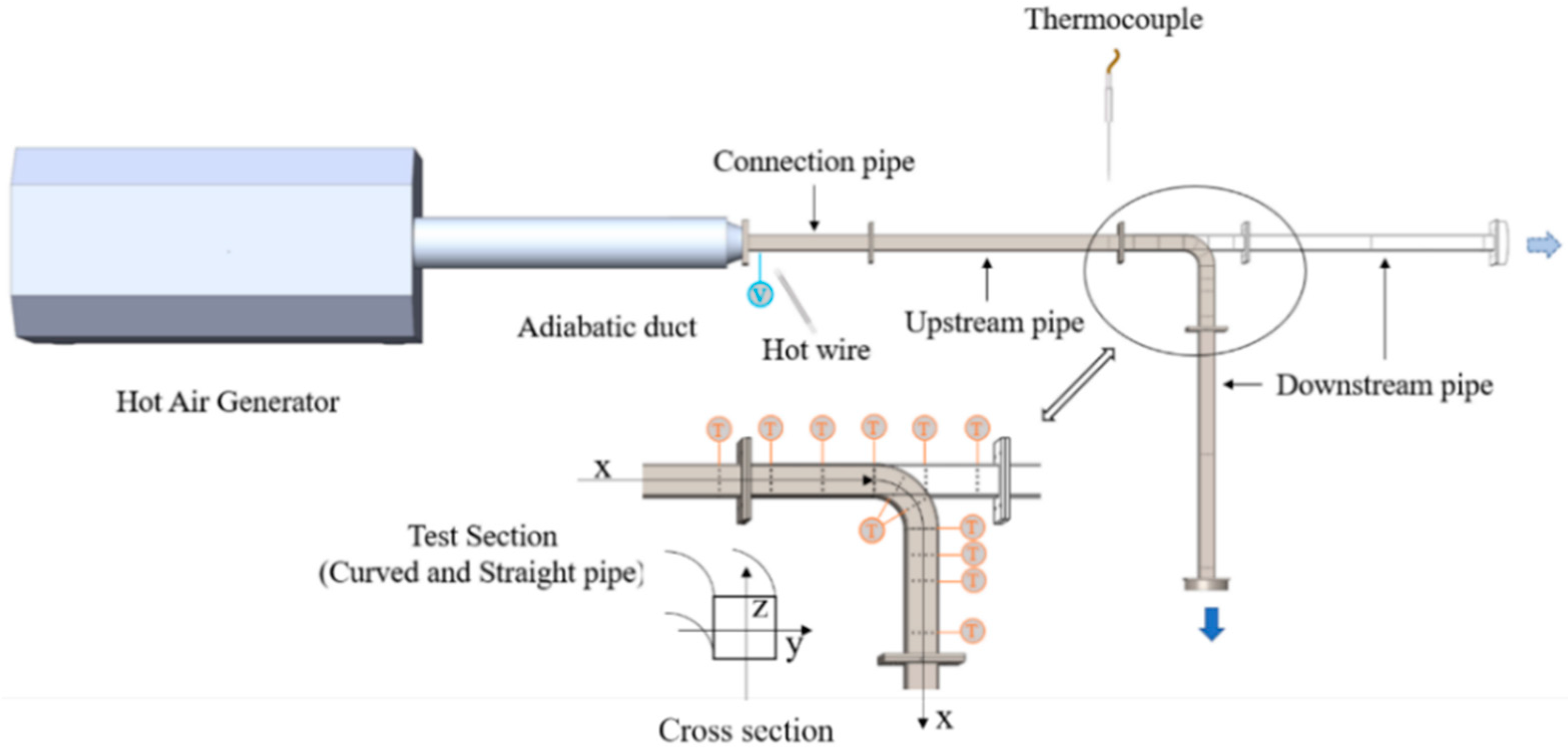
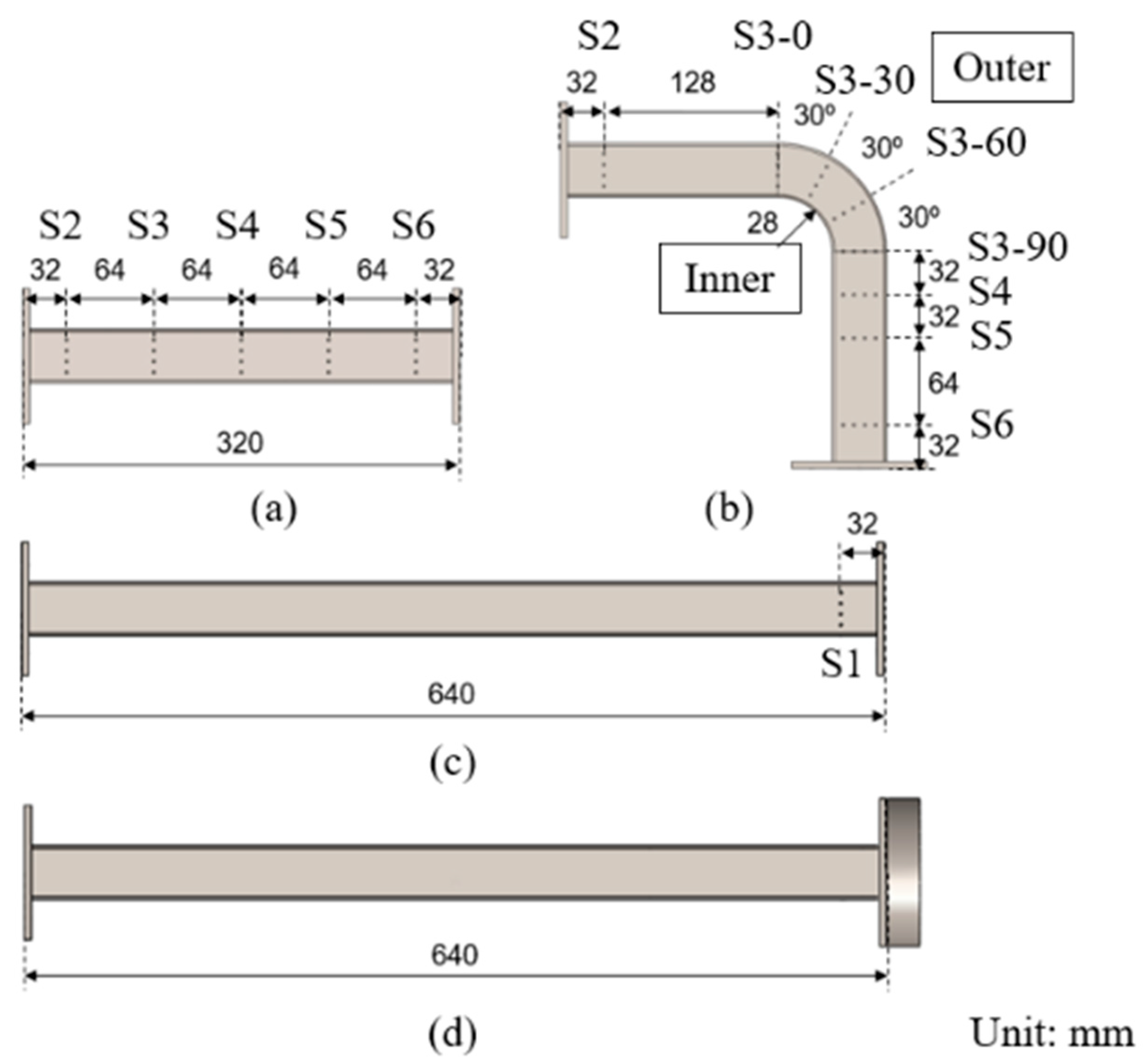
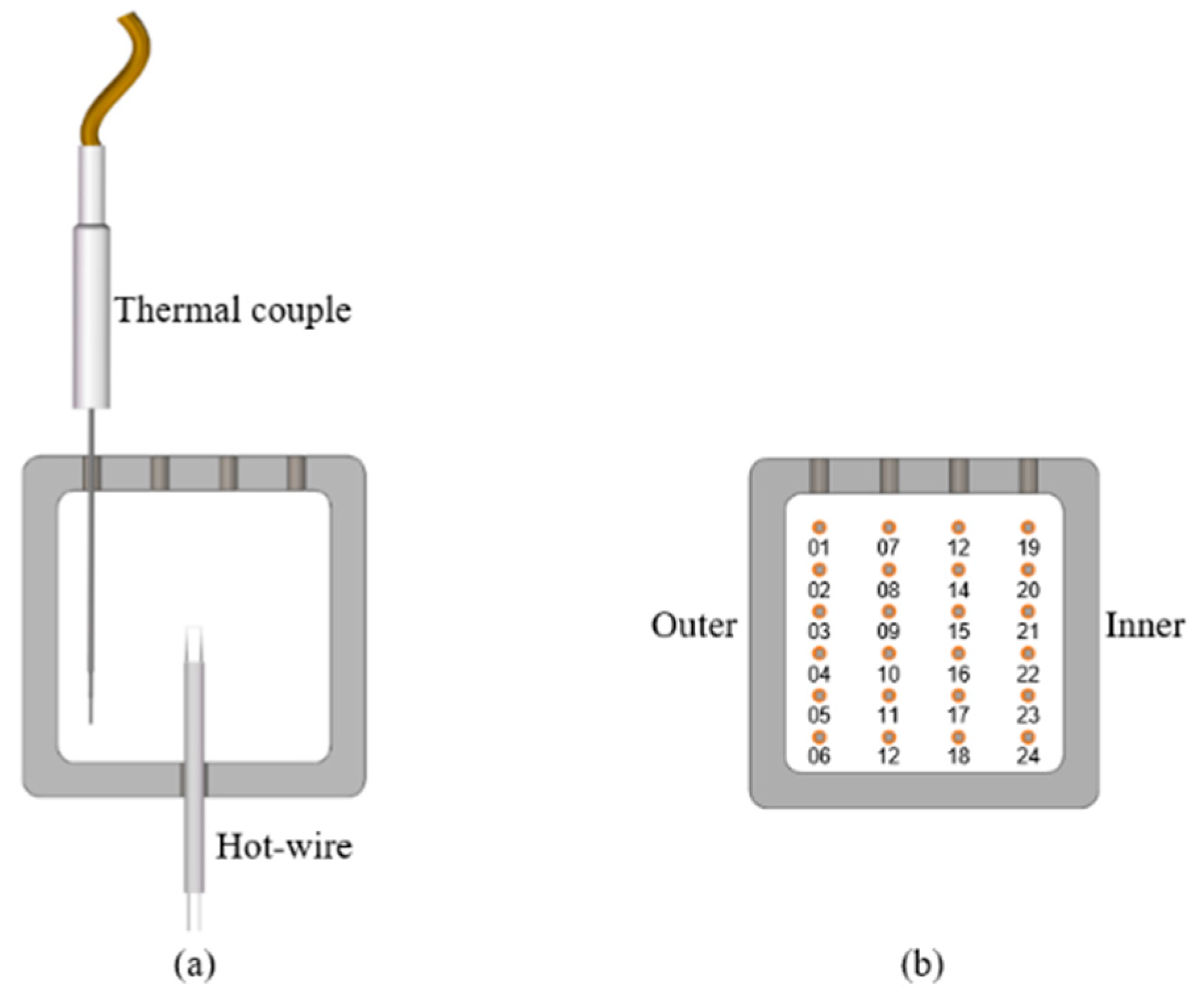
2.1. Experimental Apparatus
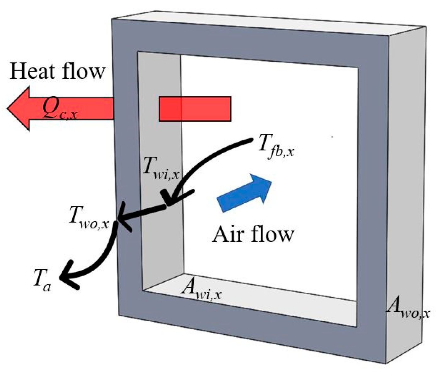
The experiment facility shown in Figure 1 was designed and constructed to investigate the effects of the curved part of the pipe on convective heat transfer. It is an open loop in which air as an operating fluid is heated by a hot air generator and passed to the atmosphere through an exhaust pipe. A hot air generator (HAP 3100, Hakko Electric, Tokyo, Japan) driven by a control panel with flow rates ranging from 2.6 to 4.6 m3/min and an air temperature ranging from room temperature to 573 K was used. Based on the proportion-integral-derivative algorithm, a hot air generator can achieve air temperature control accuracy within 1 K. The coordinate system is shown in Figure 1, where X, Y, and Z denote the streamwise direction, horizontal direction of the cross section, and vertical direction of the cross section, respectively.
After hot air passes through the adiabatic duct, the velocity and temperature of the hot air provide a uniform entrance condition at the connection square pipe. Subsequently, the hot air passes through the test section via the upstream square pipe and then the exhaust pipe after being passed through the downstream square pipe. The hot air enters the test section at a uniform temperature and develops turbulence after the connection and upstream pipes.
The schematic diagrams of the test square pipes are shown in Figure 2. The pipes were manufactured using SUS 304 with an inner diameter of 32 mm and an outer diameter of 40 mm. Fifty-six holes with a diameter of 2 mm were drilled on the top surface of the pipes. These 56 holes were used for thermocouple insertion to measure the cross-section hot-air temperature. A hole with a diameter of 5 mm was drilled on the bottom surface of the upstream pipe such that a hot-wire anemometer (0251R-T5, Kanomax, New Jersey, USA) can be installed to measure the velocity of the hot air. A hot-wire anemometer was used after calibration with a pitot tube under a high temperature. A film thermocouple (No. 3728359, Yamari, Osaka, Japan) was used to measure the temperature outside the pipe wall. Figure 3a shows the methods to measure the velocity and temperature.
In many studies, the outside of the pipe is wrapped with an electric heater to achieve a constant heat flux wall condition. In the present study, because multiple points of temperature inside the pipe must be measured, no heater was wrapped outside the pipe. In fact, many heat exchangers are directly exposed to the environment. Therefore, the outside of the pipe can be considered as a free convection heat transfer condition.
T-type thermocouples (T35, Okazaki, Kobe, Japan) were used to measure the hot air temperature of each cross-section. As shown in Figure 3b, each section comprised 24 temperature measurement points, in which the straight and curved pipes had six and nine temperature measurement cross-sections, respectively.
For the convenience of description, the temperature measurement points of each cross section were numbered from 01 to 24, as shown in Figure 3b. The first measurement section on the outlet of the upstream pipe was defined as the origin. For the straight pipe, S1–S6 represent the six cross-sections measured. For the curved pipe, the four sections of the 90° curved part were numbered by S3-0, S3-30, S3-60, and S3-90. The remaining cross-sections were numbered by S1, S2, S4, S5, and S6, as shown in Figure 2.

2.2. Data Reduction

To visualize the heat transfer process, a schematic diagram of the pipe heat transfer was drawn, as shown in Figure 4. Heat flow occurred from the high-temperature air inside the pipe through the pipe wall to the ambient.
The local heat flow rate (Qc,x) was calculated using the following equation:
Q c , x = h o A w o , x ( T w o , x T a ) ,  
where ho is the local heat transfer coefficient of the outside wall of the pipe. For the free convection heat transfer wall boundary condition of the outside wall of the pipes, the typical value of the heat transfer coefficient ranges from 2.5 to 25 W/m2·K [32]. The heat transfer coefficient significantly affected the temperature distribution in the simulation. After calibration using both the experiment and the simulation results of the temperature fields, the heat transfer coefficient was selected as 14 W/m2·K. In Equation (1), Awo,x is the local outside wall area of the pipe, Two,x is the local outside wall temperature of the pipes, and Ta is the far-field ambient temperature.
Based on the heat transfer process through the cylinder wall, the heat flow rate was constant in the fluid flowing in the pipe to the inner wall of the pipe, the inner wall to the outer wall of the pipe, and the outer wall of the pipe to the ambient fluid. The local inner wall temperature (Twi,x) can be calculated using the following heat conduction equation:
T w i , x = Q c , x x λ s A w , x + T w o , x ,  
where ∆x is the thickness of the pipe (4 mm), Aw,s is the average of the local outside wall area (Awo,x) and inner wall area (Awi,x), and λs is the heat conductivity of the pipe.
The local Nusselt number is defined by:
N u , x = h i , x D λ f ,  
where λf is the heat conductivity of the fluid in the pipe, and D is the characteristic length. D is the same as Din in the present study. hi,x is the local heat transfer coefficient of the inner wall of the pipe, which can be calculated using the following equation:
h i , x = Q c , x A w i , x ( T f b , x T w i , x ) ,
where Awi,x is the local inner wall area of the pipe. Tfb,x is the local fluid bulk temperature across the sections of the pipe, which can be obtained from the average value of the local cross-section temperatures.
The measurement accuracies of the major parameters used are shown in Table 1.

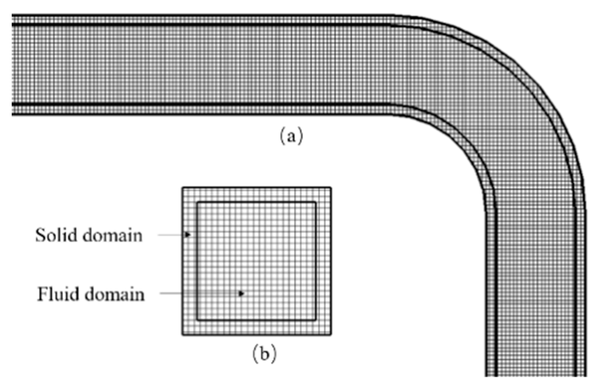
3. Formulation and Numerical Methods

The numerical simulations were performed using CONVERGETM (Convergent Science, Wisconsin, USA) computational fluid dynamics software. Under the same conditions as in the experiment, the CHT method was used to solve the flow and heat transfer in both the solid and fluid regions.
The computational domain comprised an upstream pipe, a test section (curved pipe/straight pipe), and a downstream pipe. The entire computational domain was discretized with a rectangular mesh, and a modified cut-cell Cartesian mesh generation method was used on the geometry surface. The mesh details are shown in Figure 5. The mesh size was 1.6 mm. As reported by Oki et al. [9], almost the same gird also used in their curved pipe simulation. The numerical velocity fields result is in broad agreement with the experimental data obtained by PIV measurement.
The three-dimensional governing equations for the density, velocity, and temperature of flow were solved using the implicit time discretization method in finite volume form on a collocated grid. For the CHT simulation, the temperatures and heat fluxes of the solid and fluid regions were consistent across the entire area of the interface boundary. The interface boundary specifies the demarcation of the solid and fluid regions.
The RNG k–ε turbulence model was used to manage turbulent flows. Furthermore, the law of the wall was applied for the velocity on the solid walls because the RNG k–ε model failed to resolve the region in the vicinity of the wall. For the temperature law of the wall boundary condition, the model reported by Han and Reitz [33] was used to account for compressible effects in a pulsating flow. The turbulent heat flux on the inner wall was modeled as follows:
λ d T d n = { ρ u τ c p ( T f T w ) y + P r m ,     y + < 11.05 ρ c p u τ T f ln ( T f T w ) 2.1 ln ( y + ) + 2.513 ,     y + 11.05 ,  
and:
y + = ρ u τ y μ m ,  
where λ is the heat conductivity, n the normal direction to the wall surface, Prm the molecular Prandtl number, ρ the density of the fluid, Tf the fluid temperature, Tw the wall temperature, and uτ the shear speed expressed as:
u τ = c μ 1 4 k 1 2 ,  
where cμ is the model constant (0.0845) from the k–ε model, and k is the turbulent kinetic energy.
In this study, the Reynolds number is defined as follows:
R e = U D ν ,  
where U is the time-averaged streamwise velocity; D is the hydraulic diameter of the pipe, which is the same as Din in the present study; ν is the kinematic viscosity of the fluid.
The Dean number used to characterize curved flows was first proposed by Dean (1959), and it is expressed as follows:
D e = R e D 2 R c   ,  
where Rc is the radius of curvature of the curved pipe, as shown in Figure 2b. The Dean number is the ratio between the centrifugal and viscous forces. For low Dean numbers (De < 40), flow is unidirectional. Some wavy perturbations are generated as Dear number increases (40 < De < 75). At high Dean number (De > 75), Dean vortices become stable.
The Prandtl number is defined as:
P r = c p μ λ ,  
where Cp is the specific heat of fluid; μ is dynamic viscosity. The Prandtl number is the ratio between momentum diffusivity and thermal diffusivity. For small Prandtl number (Pr << 1), the heat diffuses faster than momentum. The temperature boundary layer is greater than the velocity boundary layer. While for large values (Pr >> 1), the momentum diffusivity dominates the flow behavior, thus, thickness of velocity boundary layer becomes much larger than the one of temperature boundary layer. However, Pr of the air considered in the present study is 0.72, which is different from extremely large and small Prandtl numbers.
The inlet boundary conditions for the velocity and temperature were obtained experimentally. The inlet velocity and temperature were measured by hot-wire and thermocouple separately. The outlet boundary condition was set at an ambient pressure of 101.325 kPa. The interface wall boundary condition was used on the inner wall of the pipe, which is the surface between the solid and fluid domains. The temperatures and heat fluxes of the solid and fluid domains were consistent across the entire area of this interface boundary. For the fluid domain side of the interface wall boundary, the velocity and temperature law of the wall were applied. No-slip wall boundary condition was used for the solid domain side of the interface wall boundary. The convection boundary condition for temperature was applied to the outer wall of the pipe. The far-field temperature was 298.15 K, and the heat transfer coefficient of this boundary was determined to be 14 W/m2·K, as the present simulation was consistent with the experiment. Furthermore, this value fitted well in the range of the free convection heat transfer coefficient. As for the experimental and numerical conditions, the temperature of the inlet condition was set at 402 K. The Reynolds number was 6.0 × 10⁴ in straight pipe and 5.9 × 10⁴ in curved pipe. Dean number was 3.1 × 10⁴ in curved pipe.
The Grashof number is the ratio between the buoyancy and viscous forces acting on a fluid. In pipes, it is expressed as:
G r = g β ( T f T w ) D 3 v 2 ,
where g is the acceleration of gravity. Grashof number is around 6200 in the present experimental conditions, which is much less than Re. Thus, the buoyancy force can be ignored in the present study.

4. Results and Discussion

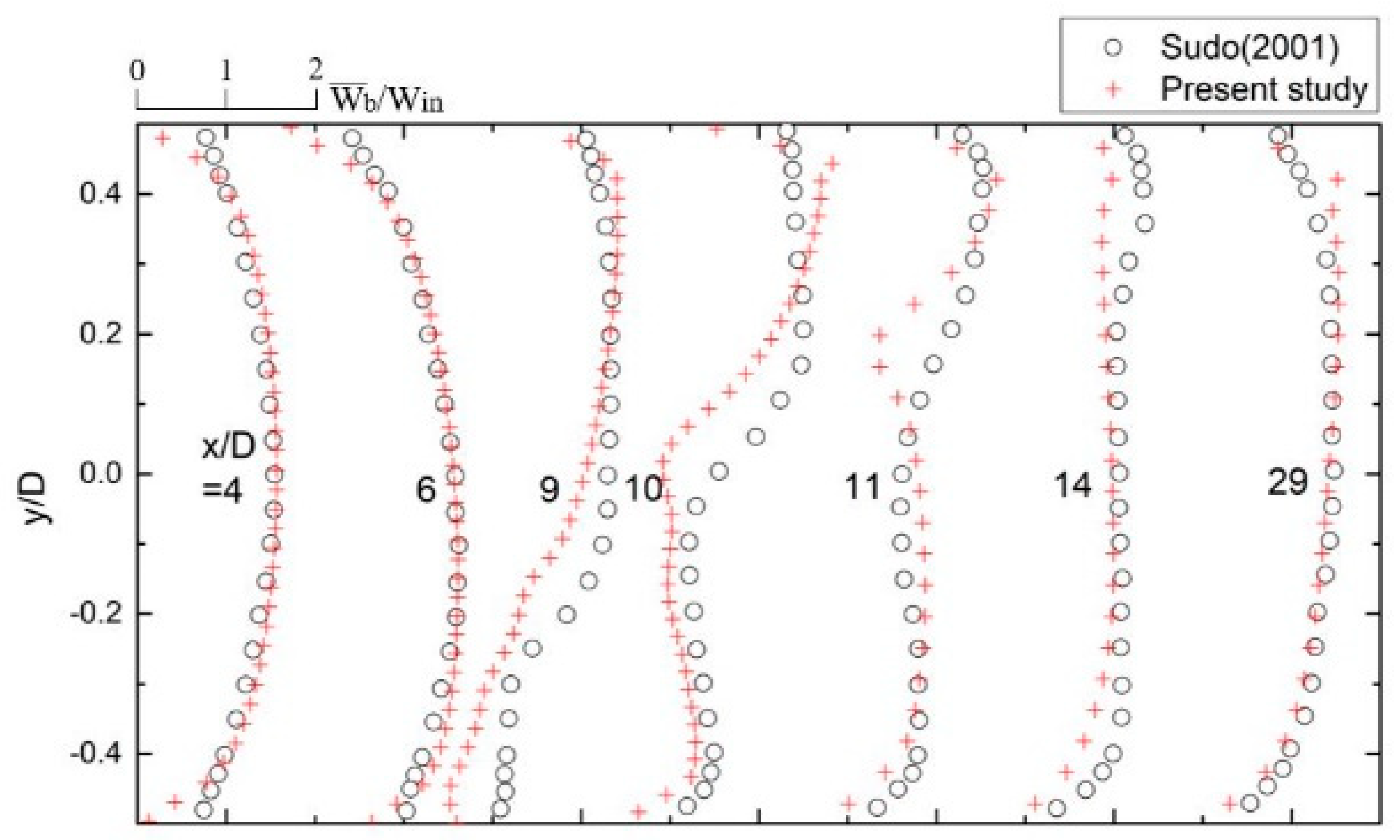
4.1. Numerical Validation for Flow Velocity

At the beginning of our investigation, our model and simulation setup were first validated against the existing experimental and numerical data reported by Sudo et al. [34] and Kim et al. [35]. Various turbulence models, such as the standard k–ε, RNG k–ε, k–ω SST, and LES were used by Kim to simulate a circular-sectioned 90° curved pipe. Based on the experimental data of Sudo et al. [36], the RNG k–ε turbulence model yielded better results for the primary streamwise velocity and the secondary swirling velocity profiles compared with other turbulence models. Sudo et al. investigated a turbulent flow in a 90° section of a curved square duct at a Reynolds number of 4 × 10⁴ using a hot-wire anemometer. Figure 6 shows a comparison of the longitudinal mean velocity distribution between Sudo et al. and the present study. The abscissa “X/D” is the streamwise dimensionless length. The origin of X/D is defined at S1; D is the inner diameter of the pipe.
The upstream and downstream of the curved pipe agreed well with the experimental results of Sudo et al. These results obtained using law of the wall have indicated that first mesh above the wall is considered to be inside the inertial sublayer (logarithmic region) on the whole, thus, the mesh used in the present study could indirectly deal with flow structure including steady turbulent boundary layer. In the curved part (X/D = 6–9), the velocity distribution of the present study differed slightly from that of Sudo et al. The curvature ratio in the geometric model and the Dean number might have contributed to this slight difference. The curvature ratio was 4 in the study by Sudo et al., but it was 3 in the present study. Meanwhile, the Dean number was 2 × 10⁴ in the study by Sudo et al., but it was 3.1 × 10⁴ in the present study. Therefore, the velocity change was more significant in our study.

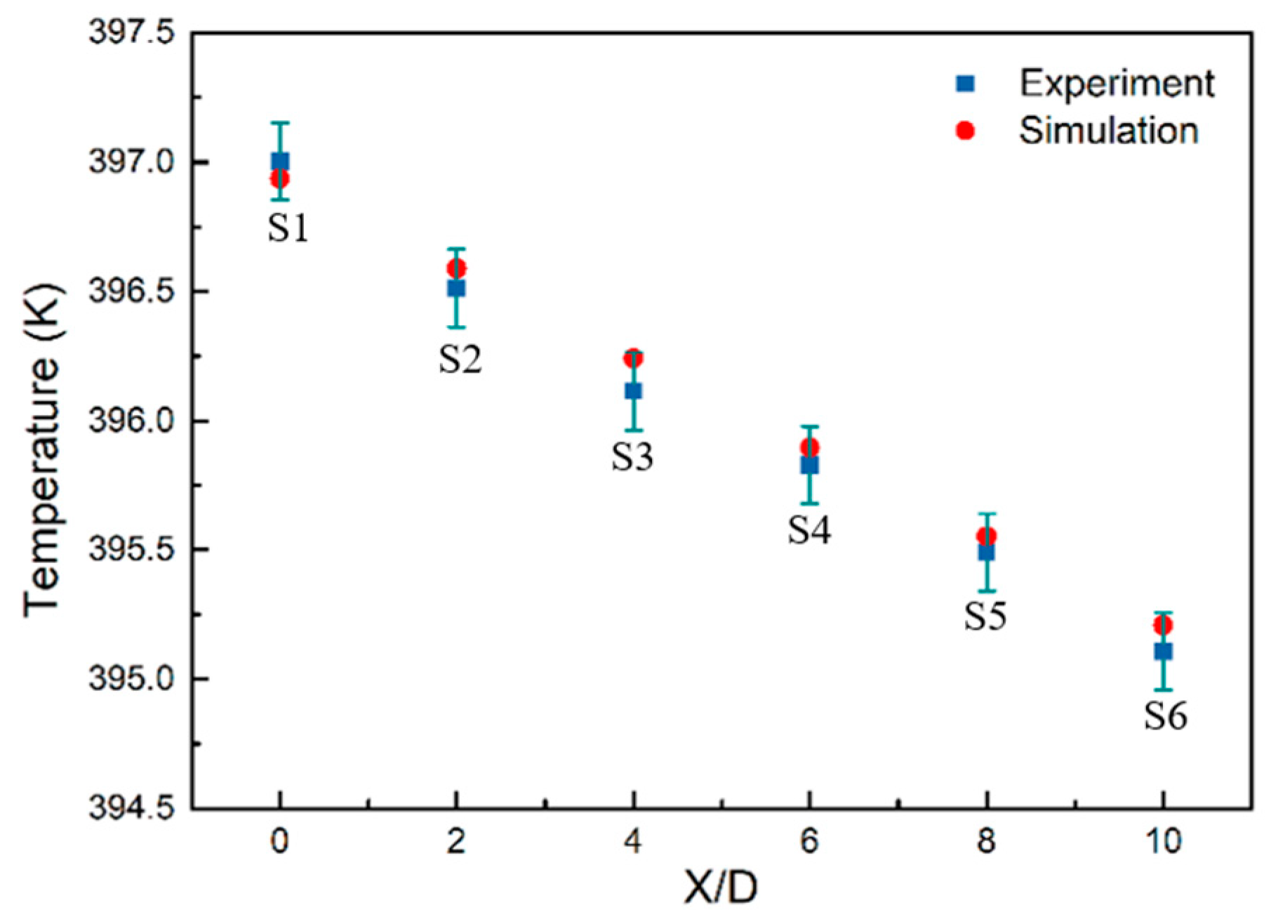
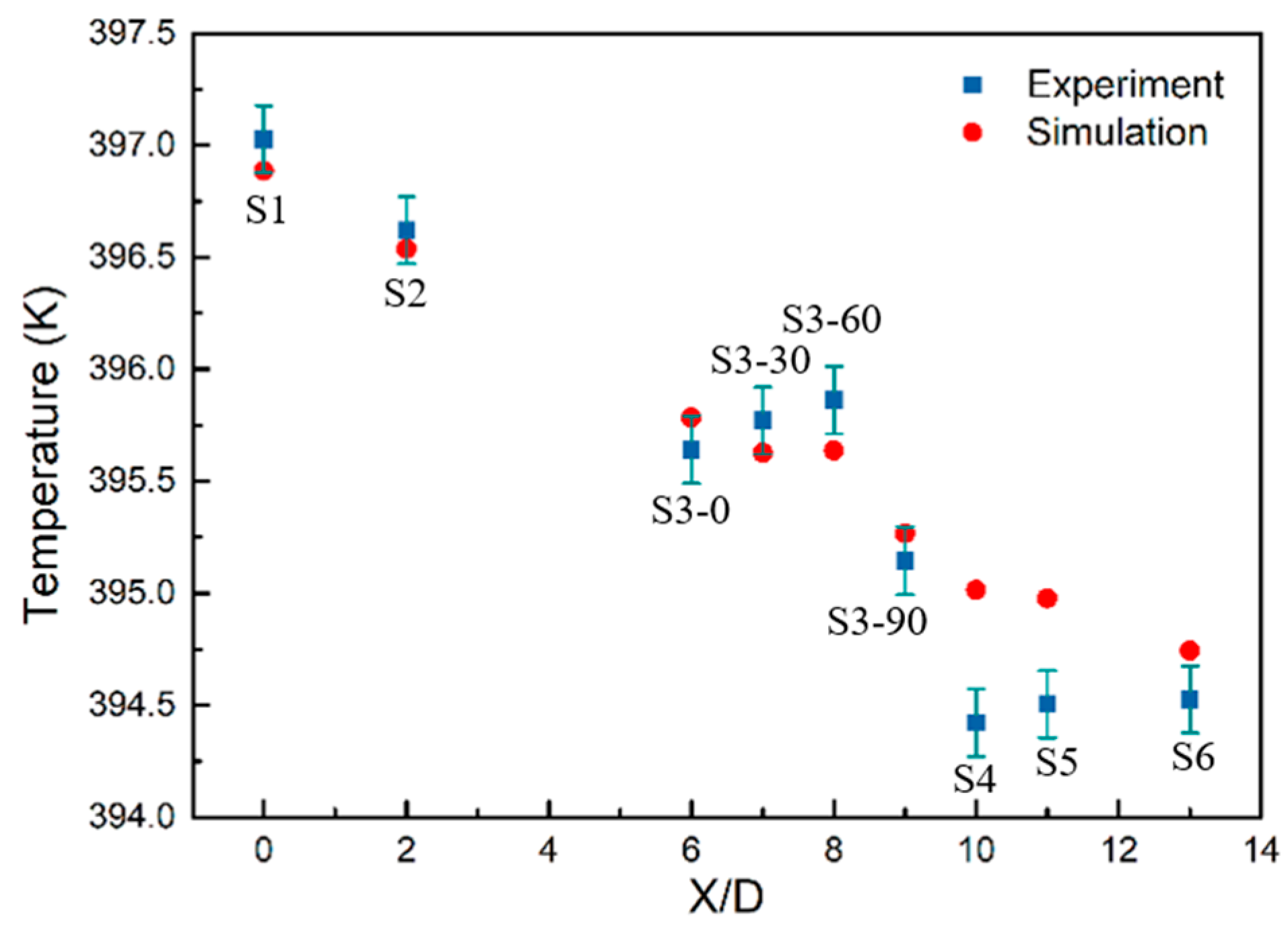
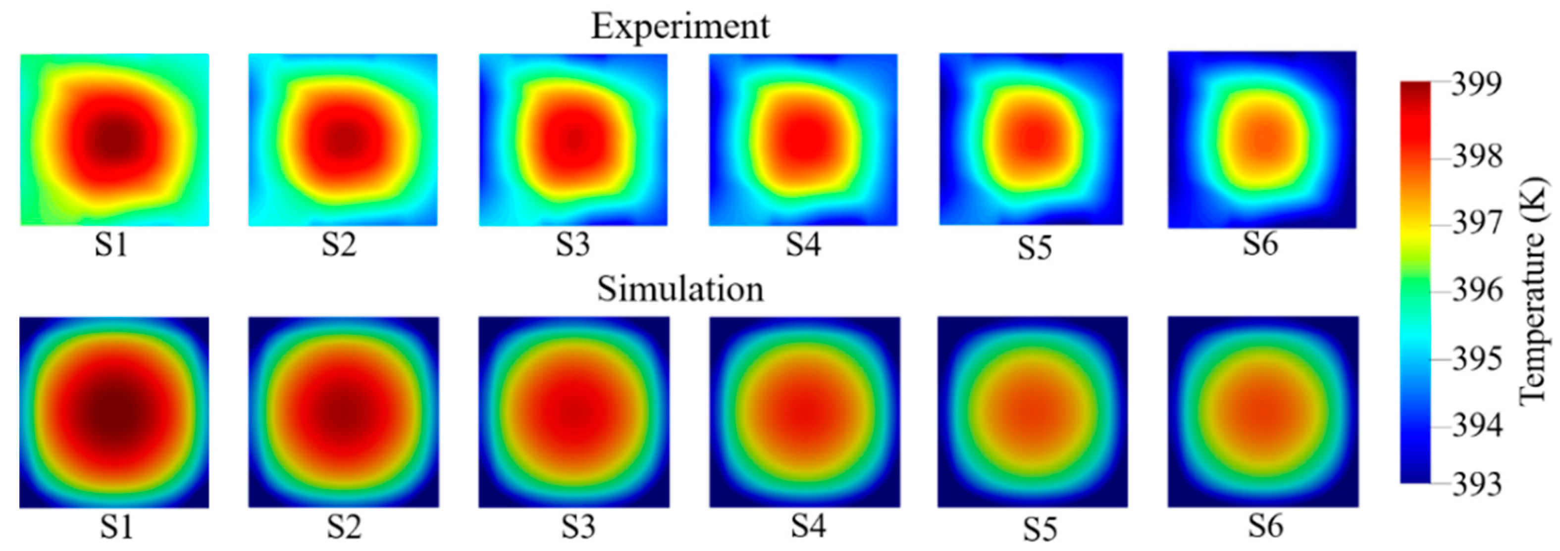
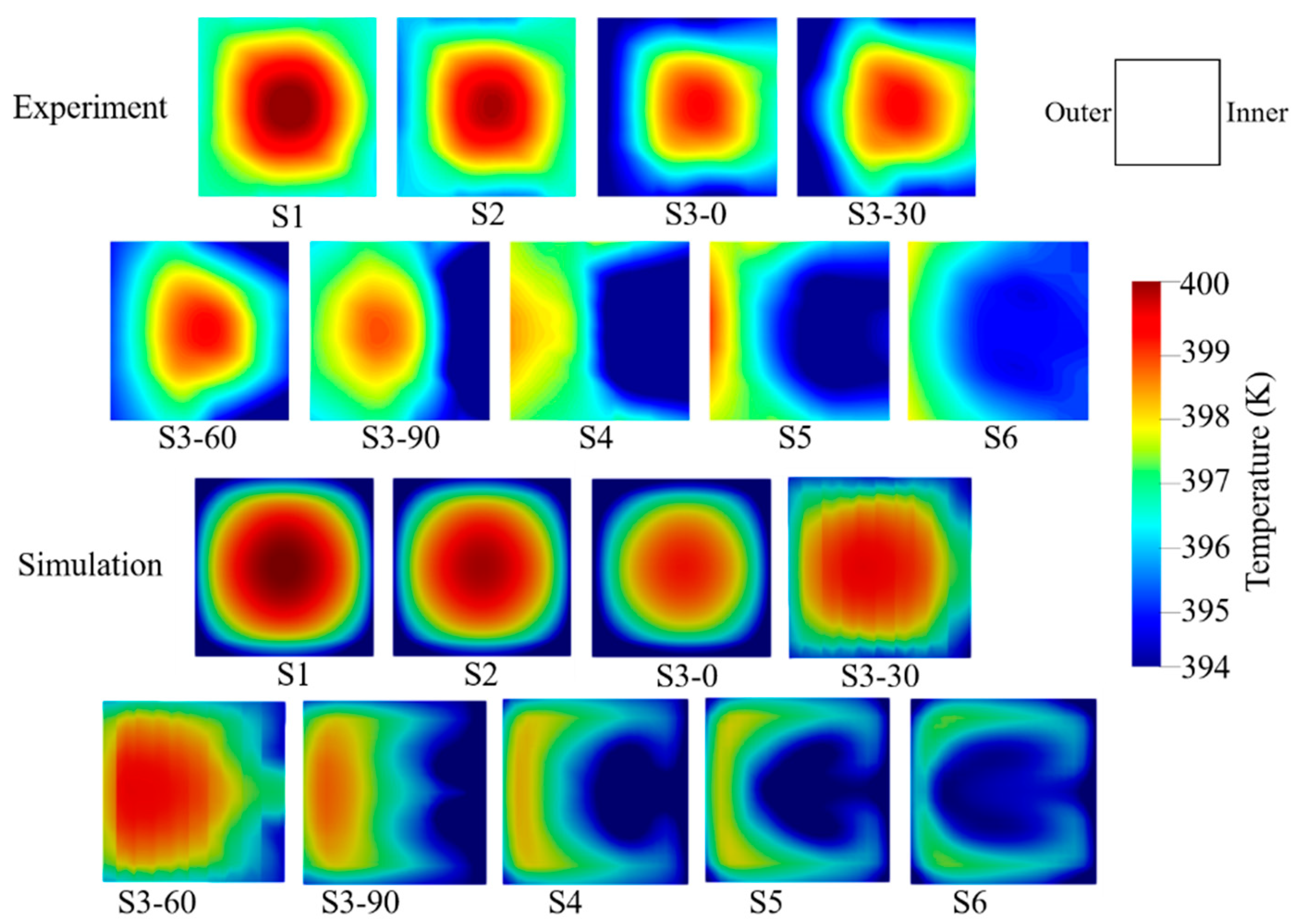
4.2. Comparison of Fluid Temperature between Experiment and Simulation

Based on 24 measured points of each cross section, the average space temperatures at the straight and curved pipe cross-sections obtained via experiment and simulation are presented in Figure 7 and Figure 8, respectively. The temperature at each measurement point was a 10-s time-averaged value. The error bar of the experiment shows the uncertainty of the hot-air temperature measurement.
As shown in Figure 7, the average temperature of the cross sections of the straight pipe decreased along the streamwise direction. Both the experiment and simulation indicated a linear trend, and they agree well with each other.
For the curved pipe, as shown in Figure 8, the average temperature of the cross sections with streamwise development showed different phenomena. The temperature decreases at S1 and S2 and it became almost constant at S3-0 to S3-60 of the curved part. Finally, it decreased significantly again at S3-90 and S4 of the downstream pipe, immediately after the curved part. The difference between the experiment and simulation became more evident in the curved part. This is attributable to the measurement error because the heat transfer coefficient of the wall was not constant in the experiment. A previous experimental study [10] indicated the non-uniformity of the heat transfer coefficient of the curved pipe on the wall surface. Although the experiment and simulation results differed slightly, their overall tendency was identical.
In the circumferential direction of the temperature fields, color contours of temperature for the experiment were created using MATLAB (MathWorks Inc., Natick, MA, USA) codes. Color contours of temperature for the simulation were obtained from CFD post-processing. Figure 9 and Figure 10 show the temperature contours of the straight and curved pipes, respectively.
In Figure 9, the temperature contours in the upper part represent the experimental results obtained using the MATLAB code, whereas the lower part represents the simulation results obtained through CFD post-processing, for a straight pipe. To facilitate the comparison of the air circumferential temperature distribution, the solid part in the simulation was disregarded. From S1 to S6, both the experimental and numerical temperature contours show a concentric circle distribution, and the temperature decreased along the streamwise direction. Owing to the significant temperature gradient at the boundary layer, the limited experimental data at the boundary layer caused the temperature from the numerical results near the solid wall to be lower than that from the experimental results.
A comparison of the experimental and numerical results of the curved pipe is shown in Figure 10. The temperature fields changed significantly at the curved part comparing with the temperature fields variation in the straight pipe. Owing to the centrifugal force, from S3-30 to S6, the high-temperature core shifted to the outer side. After the pipe curvature, along with the secondary flow generation, the temperature field gradually formed a typical symmetric vortex distribution.
The main differences between the experiment and simulation can be observed at S3-0 and S3-30. In the experiment, the temperature of the inner side was higher than that of the outer side. By contrast, in the simulation, the temperature of the outer side was higher. This phenomenon was caused by the geometry of the curved pipe. In the experiment, since our pipe was not surrounded by heaters but directly exposed to the environment, the downstream part of the curved pipe with high temperature resembled a “heat source.” In the geometry, for the curved part of the curved pipe, this “heat source” was located near the inner side and away from the outer side. Hence, this “heat source” can increase the ambient temperature just above the inner side wall, causing a decrease in the normal gradient of temperature toward fluid on the inner wall. Therefore, the temperatures of the inner sides of S3-0 and S3-30 in the experiment were higher than those of the outer sides. In the subsequent part (from S3-60 to S3-90), as the effect of the centrifugal force was more prominent, the high-temperature core deviated and the flow impingement occurred on the outer side wall, increasing the outer side temperature.
Compared with the simulation, the secondary flow temperature distribution in the experimental results was not distinct because of insufficient temperature measurement points, particularly in the inner region formed by the secondary flow. Due to the large mesh size on the wall surface, the boundary layer information cannot be captured very well because the boundary layer thickness is thought to be thinner than base mesh size 1.6 mm in the present paper. However, this study investigated the comparison of temperature distribution between experiment and simulation for steady turbulent flows, and the current simulation results basically agree with the experimental results for temperature as well as velocity.

4.3. Numerical Investigation

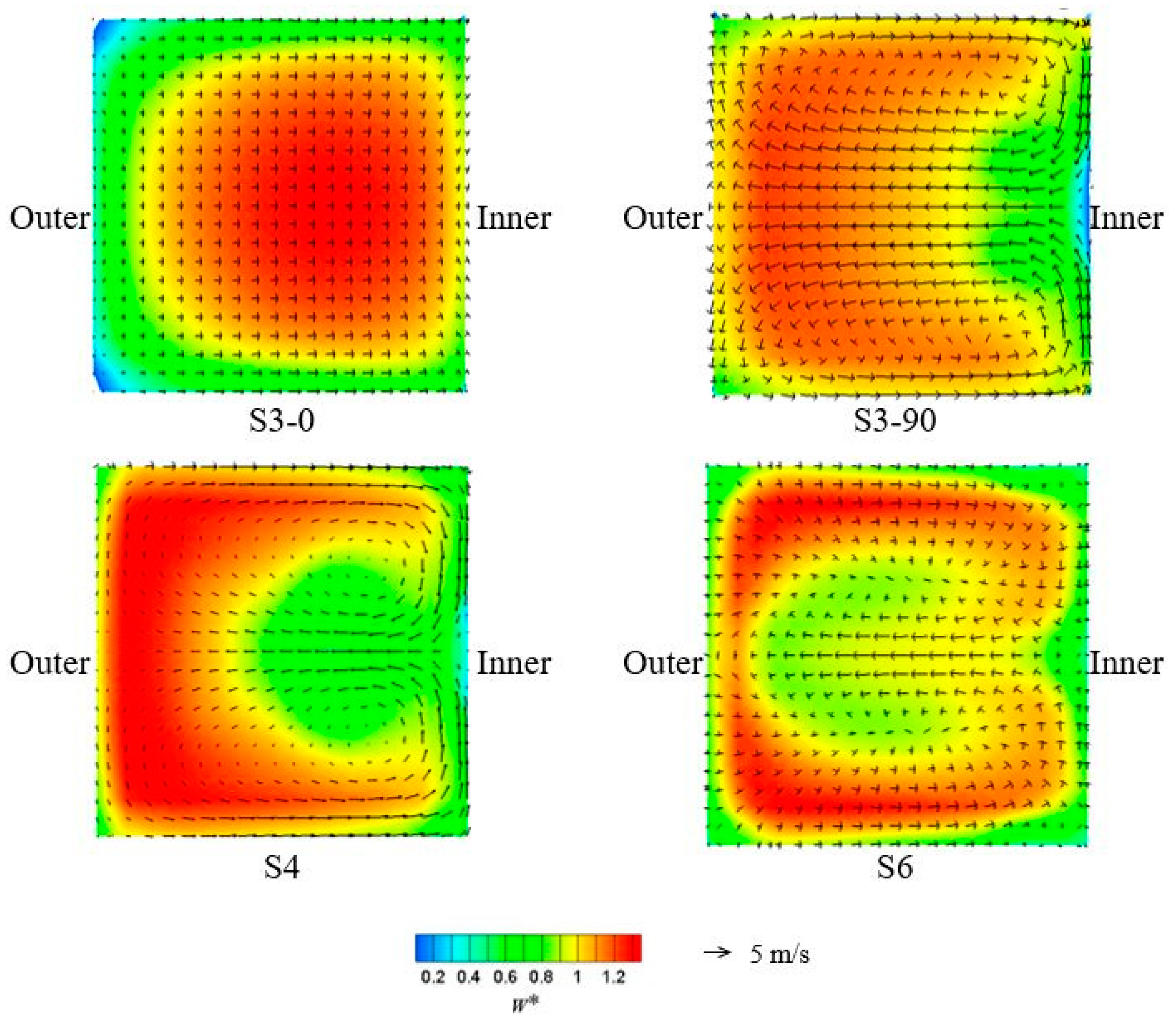
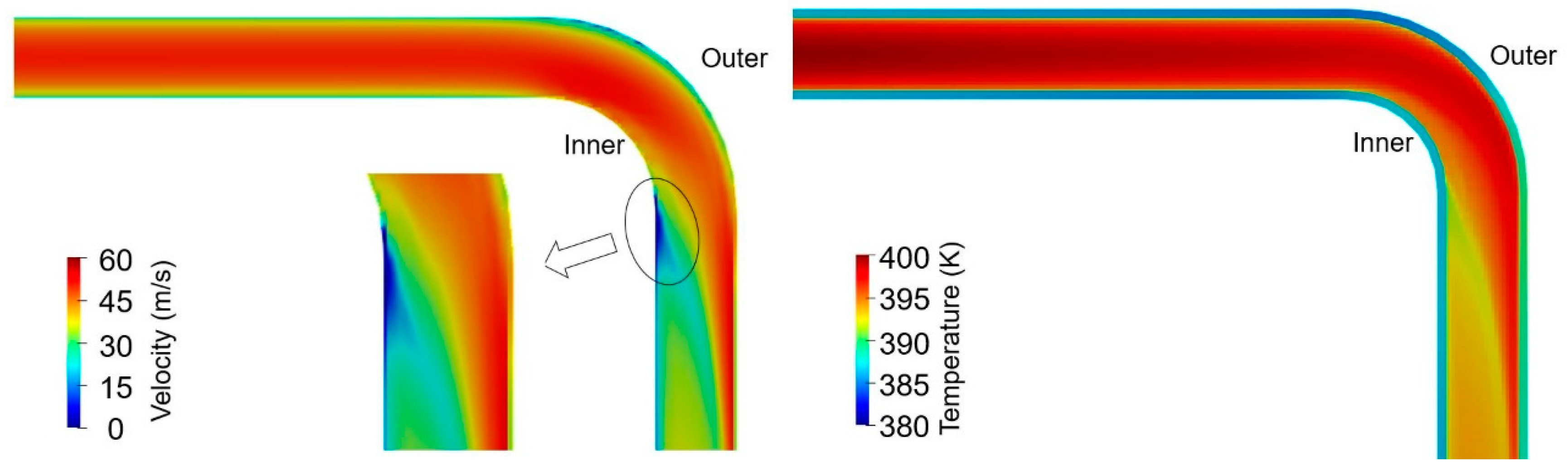
4.3.1. Time-Averaged Flow in Curved Pipe

Figure 11 shows the time-averaged results of the various cross-sections. Each of them is a combination of the vector plot of the time-averaged secondary flow resulting from the vortex flow and the color contours of the time-averaged dimensionless streamwise velocity. As mentioned previously, at the beginning of the curvature, as shown in S3-0, the high streamwise velocity core shifted to the inner side. Furthermore, the curvature affected the velocity and temperature distribution of the upstream section of the curved part. The secondary flow of the typical Dean vortex was observed in S3-90, S4, and S6. These results agreed well with the data of Oki et al. [37]. The high streamwise velocity core indicated the expected distribution from the inner to outer wall. Although S3-90, S4, and S6 exhibited the Dean vortex, the high streamwise velocity core shifted gradually to the top and bottom with the development of the secondary flow. This movement promoted the mixing of air and enhanced heat transfer performance. It is noteworthy that the streamwise velocity was extremely low at the top and bottom left of S3-0 and at the midpoint of the inner side of S3-90. As shown in Figure 10, the temperature was also extremely low at the low velocity region. The low temperature region decreased the local temperature difference between the pipe and the ambient, thereby suppressing heat transfer.
To further investigate the causes contributing to the formation of the secondary flow temperature fields in the curved pipe, a streamwise velocity and the temperature contours of the horizontal section along the center axis are shown in Figure 12. Because centrifugal force was generated, the velocity and temperature near the outer wall were significantly higher than those at the inner wall. The high-temperature core in the air flow impinged on the outer wall after the bend, as shown in Figure 12, and the outer wall temperature increased. Therefore, the heat transfer to the outside of the pipe was further enhanced by the temperature difference between the wall and the ambient.
By contrast, after S3-90, the air separated from the inner wall. This separation resulted in a significant decrease in the temperature of the air near the inner wall, and the temperature difference between the wall and the ambient decreased. Hence, heat transfer was reduced at the inner wall after the curvature. It is found that there is recirculation downstream. Recirculation occurred just after the air separated from the wall. However, the recirculation is a very small size, thus, the authors consider the recirculation hardly affects flow characteristics discussed in the present paper.
Hence, it can be concluded that flow impingement enhanced heat transfer, whereas flow separation suppressed heat transfer. This conclusion is consistent with the simulation result of Arvanitis et al. [23].

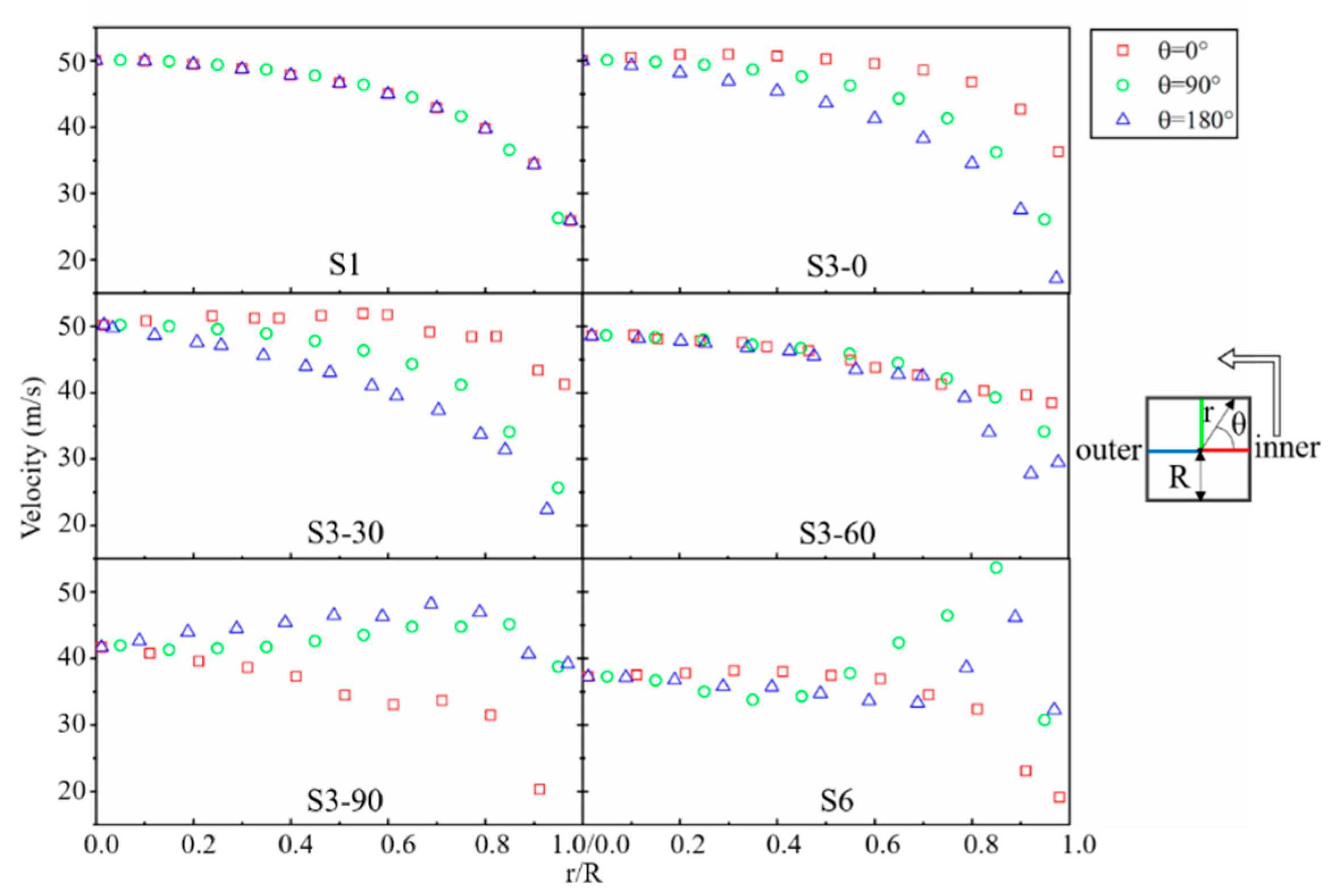
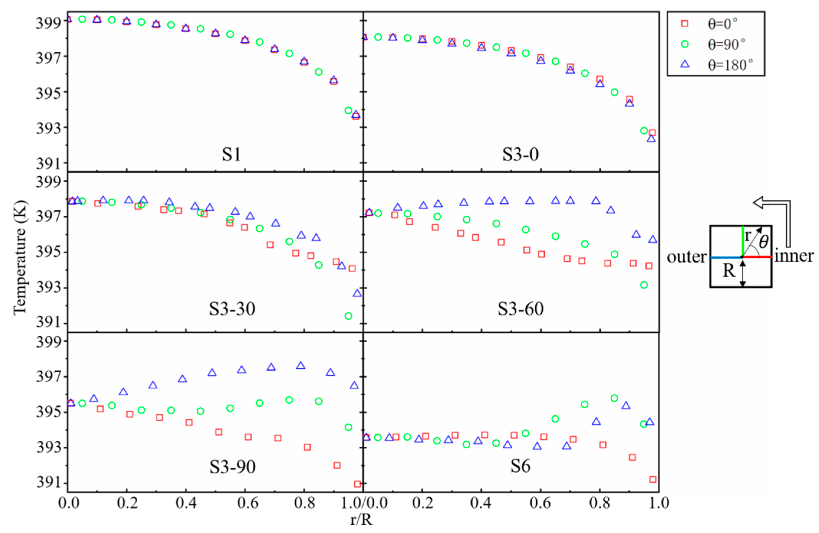
4.3.2. Radial Profiles of Velocity and Temperature for Various Cross-Sections

The detailed results for the time-averaged velocity and temperature are shown in Figure 13 and Figure 14, respectively. The profiles of velocity and temperature along with different radial directions (from the pipe center to the inner, upper, and outer walls) for various cross-sections are depicted. The three radial directions are defined as θ = 0°, 90°, and 180°. The coordinate r is the radial coordinate in the cross section, and R is the pipe inner radius. For S1, regardless of the temperature and velocity, the three radial (θ = 0°, 90°, and 180°) profiles were identical because this cross section was in the straight pipe that was upstream of the curvature, and both the velocity and temperature in the cross section were symmetrical in the pipe. At S3-0, the difference between the velocity and temperature began to appear, and the three radial velocity profiles changed. As the angle of θ increased from 0° to 180°, the velocity decreased gradually. The velocity near the inner side was much higher than that on the outer side. This result is consistent with Figure 12. However, the temperature profile remains almost unchanged, consistent with the distribution of S1. It is noteworthy that studies about the heat transfer performance of a curved pipe are not limited to the velocity field inside the pipe, but also the temperature field inside the pipe.
At the curved parts (from S3-30 to S3-90), the velocity and temperature for θ = 180° began to increase gradually. However, the velocity and temperature for θ = 0° began to decrease significantly. During this process, the velocity and temperature profiles no longer exhibited a monotonous decreasing trend from the center to the edge; instead, a local countertrend appeared. This was primarily due to the centrifugal force, which caused the high temperature and high velocity core to deviate and collide with the outer wall of the pipe; the secondary flow contributed to the phenomenon as well. The phenomenon was observed the most clearly in downstream straight pipe part S6 after the curved part. Owing to the full effect of the secondary flow, the temperature and velocity profiles differed significantly from those of S1. In S6, the temperature and velocity fields near the upper wall and outer side wall were larger than those at the center.

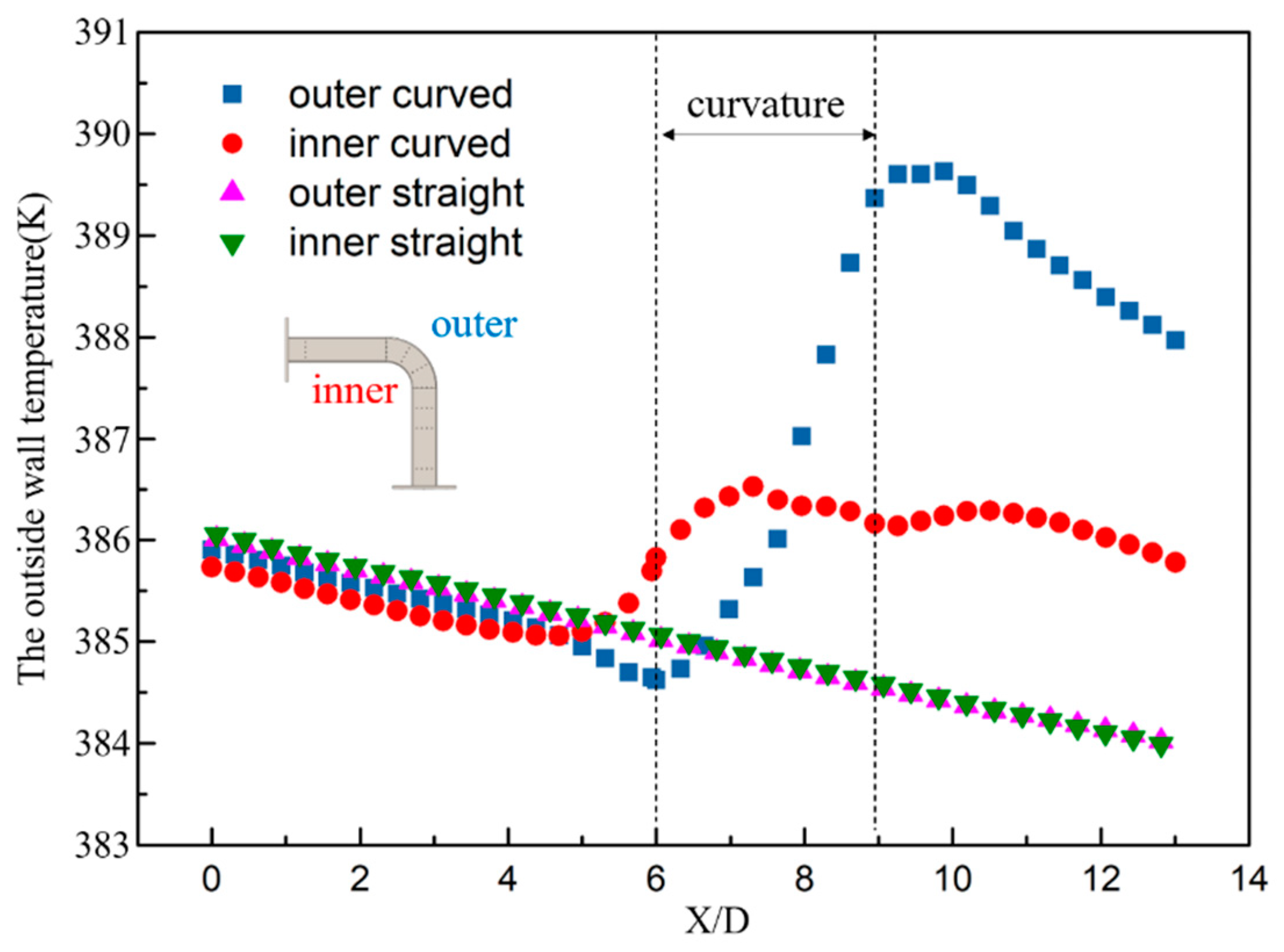
4.3.3. Outside Wall Temperature Distributions

CHT simulation can solve flow and heat transfer in both fluid and solid regions simultaneously. Because of the thickness of the pipe wall, there is a temperature difference between the two sides of the pipe wall. In present study, hot gas passed through the pipe, and it is difficult to measure the inner wall temperature in the experiment. The outside wall temperature was easily measured and compared with CHT results. Thus, we used CHT simulation. Compared to other approximations, CHT has the advantage of displaying solid region information. Because the heat transfer of the solid region can be solved using the heat conduction formula, it is more concise and simpler than that of the fluid region.
The streamwise temperature variations of the inner and outer wall middle points of the solid region are shown in Figure 15. The temperature variation tendency of the solid wall was similar to that of the fluid. Both the temperatures on the inner and outer walls of the straight pipe decreased in the streamwise direction, whereas their temperatures were similar.
The temperature variations of both the inner and outer walls of the curved pipe indicate different behaviors: both the outer and inner temperatures oscillated, particularly in the curved part of the curved pipe. Before the curvature, the outer temperature decreased slightly, whereas the inner temperature increased, as shown from S2 to S3-0 in Figure 10, in which the high-temperature core shifted slightly toward the inner side. In the curved part, owing to the flow deviation and impingement, the thermal boundary layer was broken, and the high-temperature core was impinged on the outer wall. Hence, the outer wall temperature continued to increase. As shown in Figure 12, the velocity near the inner wall was high. This high velocity with high momentum can break the thermal boundary layer. As shown in Figure 10, from S3-30 to S3-60, the thermal boundary layer in the middle of the inner wall was in fact broken by this high velocity. Therefore, the temperature of the inner wall increased at the initial curvature of the curved pipe.
As the velocity near the inner wall decreased, along with the separation effect, the inner temperature decreased gradually. After the curvature, the deviation effect of the high-temperature core caused by the centrifugal force weakened gradually, causing the thermal boundary layer of the outer wall to be repaired again. Consequently, the temperature on the outer side indicated a downward trend. The formation of the secondary flow near the inner wall continued to evolve, increasing the gas mixing. The secondary flow vertical structures transferred the air from the top and bottom to the middle, causing a brief increase in the inner temperature after the curved part.

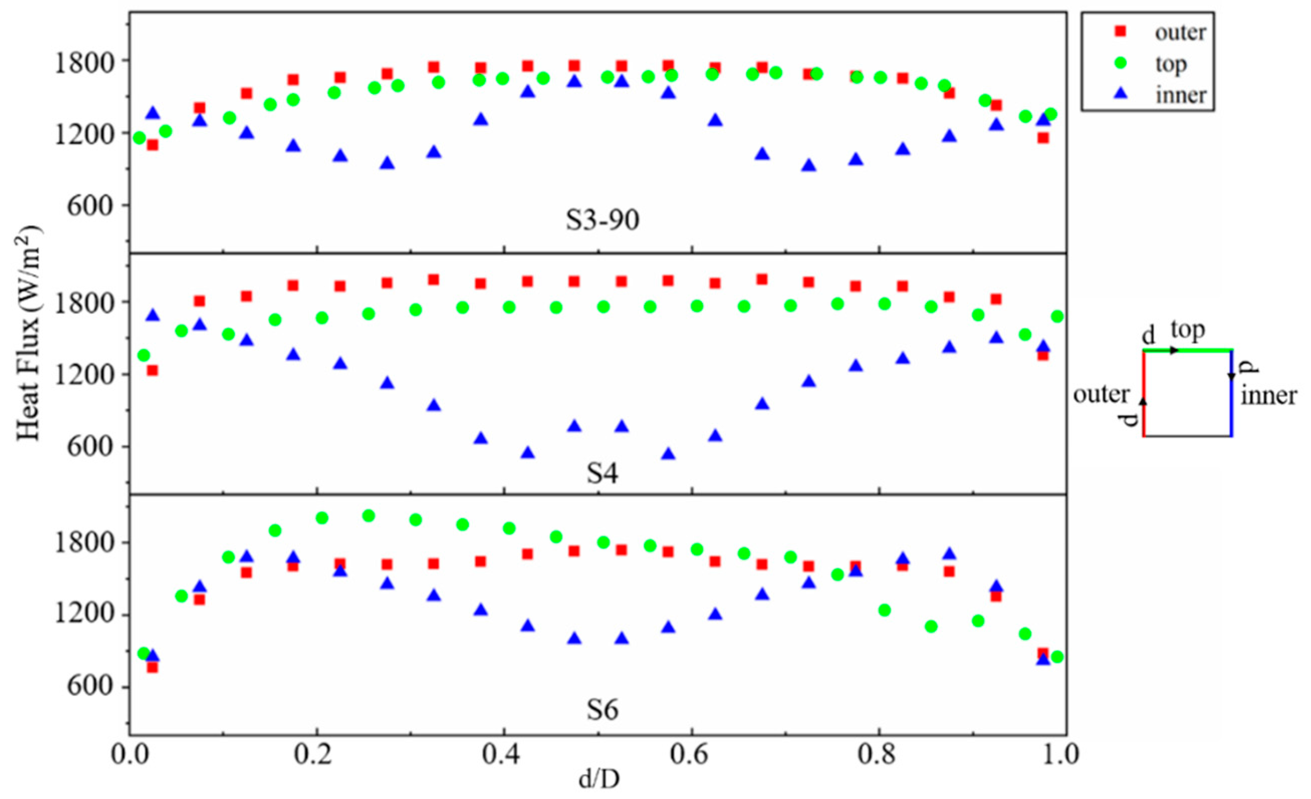
4.3.4. Wall Heat Flux Inside the Pipe

Heat flux is an important parameter that reflects the heat transfer performance. Based on our investigations, in both the straight and curved pipes, the flow and temperature distributions indicated a symmetrical structure, and the axis of symmetry was the horizontal mid-surface of the pipe. Therefore, only the outer wall, top wall, and inner wall should be analyzed. As shown in Figure 16 and Figure 17, the numerical wall heat flux at the interface between the hot air and the solid wall of different cross-sections formulated the heat transfer more intuitively. The coordinate d is the circumference coordinate on the wall, and D is the inner diameter of the pipe. The origin of the coordination is defined at the starting point of each wall.
A typical square straight-pipe heat dissipation curve appeared in S1. The wall temperature was variable even at the same local cross section because the cross section of the pipe is square, not circular, as shown in Figure 9. For each cross section, the maximum wall temperature was the midpoint of each wall. The maximum temperature difference between the wall and the ambient was also the midpoint of each wall. Hence, the heat flux reached the maximum value at the midpoint of each wall. At the initial part of the curvature (from S3-0 to S3-30), the heat flux on the inner side began to increase, and conversely, the outer side indicated a downward trend. During this process, the effect of the centrifugal force was insufficient to break the thermal boundary layer. As mentioned above, the area on the outer side was larger than that of the inner wall. Therefore, the heat flux decreased more significantly on the outer side, whereas the opposite occurred on the inner side. The same phenomenon was observed on the top side, and the heat flux near the inner side was higher than that near the outer side.
From S-90 to S4, the heat flux of the outer side began to dominate gradually. Furthermore, owing to the formation of the secondary flow, the heat flux distribution on the top side became more uniform, and the maximum heat flux was no longer at the midpoint of the inner wall. During this process, the centrifugal force dominated, thereby destroying the thermal boundary layer of the outer wall, and the heat flux of the outer side reached the maximum level. On the contrary, on the inner wall, the heat flux indicated a decreasing trend first and then increased from the two sides to the center. For the heat flux distribution on the top side, a conspicuous change compared with the previous one occurred at the point near the inner side, in which the distribution increased instead of decreased. This is attributed to the formation of the secondary flow, which resulted in the movement of the top and bottom sides of the air. However, for S6, it was located further downstream of the curvature. Therefore, the deflection of the high-velocity and high-temperature core, the separation between the wall and air, and the formation of secondary flow gradually weakened the effect of heat transfer. Although the effects of the factors above were still applied, the average heat fluxes on the top, outer, and inner lines were similar.

4.4. Nu Number Comparison

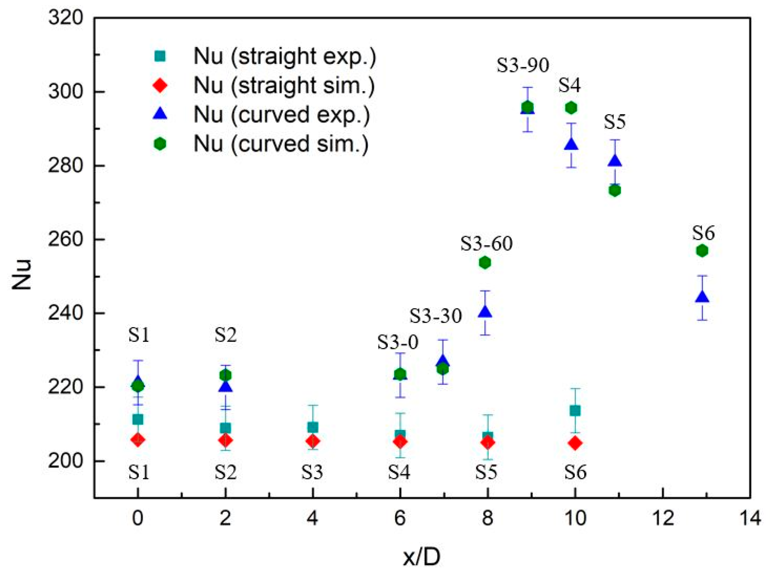
4.4.1. Total Nu Number

Many correlations exist for calculating the Nu number, particularly for straight pipes. The Dittus–Boelter empirical correlation is as follows [38]:
N u = 0.023 R e 0.8 P r 0.3         ( 0.6 P r 160 ,     R e 10 4 ,     L / D i n 60 ) ,  
Furthermore, the highly accurate Gnielinski [39] correlation is expressed as follows:
N u = ξ 8 ( R e 1000 ) P r 1 + 12.7 ξ 8 ( P r 2 3 1 ) [ 1 + ( D i n L ) 2 3 ] ( T f T w ) 0.45         ( 4 · 10 3 R e 10 6 , 0.5 P r 200 ) ,
where ξ denotes the friction factor for smooth tubes calculated from the Filonienko [40] relationship, i.e.,
ξ = ( 1.82 l o g R e 1.64 ) 2
To validate the accuracy of our approach, we compared our results with the correlations above. The deviations obtained were 31% and 18% using Equations (11) and (12), respectively. The deviation with the Dittus–Boelter correlation was slightly large owing to some constraints on the equation. For example, L/Din should be greater than 60, and the pipe should be smooth. The deviation with the Gnielinski correlation was within 20%. The Gnielinski correlation demonstrated a better agreement under the present study condition.

4.4.2. Local Nu Number

Along with the presented investigations and analysis, the observed trends indicated a more significant disruption in the temperature fields for the curved pipe. Hence, a question arises: what is the effect of the deviation, impingement, and secondary flow on the overall thermal performance of the curved pipe?
Based on the findings outlined above, we evaluated the effects of all these phenomena on the local Nusselt number in both straight and curved pipes. Figure 18 shows the variation in the circumferentially averaged local Nu for both the experiment and simulation along the dimensionless length (X/D). Because the inlet conditions of the straight and curved pipes differed slightly, the local Nu differed at the beginning of the test section (X/D = 0).
The straight pipe local Nu presented an approximately linear trend both in the experiment and simulation. However, a slightly diminishing trend appeared in the numerical simulation because the temperature continued to decrease as the fluid advanced in the downstream direction. The boundary condition between the outside solid wall and the ambient in the simulation was the free convection heat transfer condition. Because the ambient temperature and heat transfer coefficient were defined, the temperature difference between the outside solid wall and the ambient decreased, whereas the heat transfer weakened gradually. For the experimental study of the straight pipe, owing to the slightly larger temperature uncertainty on the outside of the pipe wall, although some sections indicated results that differed from the simulation results, they were still within the acceptable range; therefore, the experimental and simulation results can be considered as similar.
For the curved pipe, the results of heat flux inside the wall indicated that the heat flux in the inner and outer parts varied differently. Based on the flow deviation and impingement, along with the secondary flow formation, it was observed that the heat transfer performance improved. The local Nu increased at the curvature. The difference between the experiment and simulation was observed mainly downstream of the curvature. This may be because, in the experiment, the geometry of the curved pipe altered the heat transfer coefficient, whereas the heat transfer coefficient was constant in the simulation. The Nu on the downstream part indicated a clear discrepancy between the straight and curved pipes. However, a converging tendency was observed for the straight and curved pipes.
For quantitative analysis, at S3-90 and S4, the local Nu increased by up to 35% compared with S1. If only the average Nu of sections S1 to S6 is used to replace the average Nu of the entire pipe, then the total heat transfer performance of the curved pipe will be 20% higher than that of the straight pipe.

5. Conclusions

In the present study, both experimental and numerical investigations of turbulent forced convection in a straight pipe and a 90° curved square pipe were performed. In both the streamwise and circumferential directions, the experimental and numerical temperature field results agreed well. For the straight pipe, the cross-section average temperature in the streamwise direction decreased monotonically, whereas the circumferential temperature distribution was concentric. For the 90° curved pipe, the temperature in the streamwise direction increased at first at the initial curvature and then decreased significantly before finally increasing again. Owing to the formation of Dean vortices, secondary temperature distributions appeared in the circumferential temperature field.
Based on the analysis of the numerical time-averaged velocity fields, it was discovered that the deviation and impingement of the high-velocity air core and the formation of secondary flow strengthened heat transfer. Conversely, the separation effect suppressed heat transfer. The local discrepancies observed in the investigated positions (S1–S6) for both the straight and curved pipes were further investigated through the analysis of local distributions of velocity and temperature profiles at different radial lines. The difference in temperature distribution between the straight and curved pipes on the outside of the wall were compared and analyzed in a CHT simulation.
The numerical local heat flux of typical sections provided a more quantitative analysis of the effects, such as impingement, secondary flow, and separation. The curved pipe exhibited more complex behavior. The overall heat transfer performances of these two pipes were investigated in the last section using the local averaged Nu number. It was demonstrated that the heat transfer performance of the 90° curved pipe was 20% higher than that of the straight pipe.

Author Contributions

This is to confirm that all the authors have contributed in diverse ways at all stages of the research including research design, data collection, and data analysis; writing—original draft preparation, G.G.; writing—review and editing, Y.O. All authors have read and agreed to the published version of the manuscript.

Funding

This research received no external funding.

Acknowledgments

Thanks to the graduated Oki and Kuga, who provided preliminary help for the research. This research did not receive any specific grant from funding agencies in the public, commercial, or not-for-profit sectors.

Conflicts of Interest

The authors declare no conflict of interest.

Nomenclature

Asurface area [m2]Greek symbols
Cpconstant pressure specific [J/kg·K]λheat conductivity [W/m·K]
dcircumference coordinate on the wall [mm]ρdensity [kg/m3]
Dinpipe inner diameter [mm]θradial angel [°]
Doutpipe outer diameter [mm]uτshear speed [m/s]
DeDean number𝛏friction factor
gacceleration of gravity [m/s2]
GrGrashof numberSubscripts
hheat transfer coefficient [W/m2·K]bbulk
kturbulent kinetic energy [m2/s2]ffluid
Ltotal length of pipe [mm]ininlet
nnormal unit vectormmolecular
NuNusselt numberssolid
PrPrandtl numberwwall
Qheat flow rate [W]wooutside wall
rradial coordinate in the cross section [mm]wiinside wall
Rpipe inner radius [mm]
ReReynolds numberSuperscripts
Rcradius of curvature [mm]¯average value
Ttemperature [℃]*normalized parameter
Utime-averaged velocity [m/s]
Wstreamwise velocity [m/s]
Xstreamwise coordinate
Yhorizontal coordinate
Zvertical coordinate

References

  1. Naphon, P.; Wongwises, S. A review of flow and heat transfer characteristics in curved tubes. Renew. Sustain. Energy Rev. 2006, 10, 463–490. [Google Scholar] [CrossRef]
  2. Dean, W.R.; Hurst, J.M. Note on the motion of fluid in a curved pipe. Mathematika 1959, 6, 77–85. [Google Scholar] [CrossRef]
  3. Tunstall, M.J.; Harvey, J.K. On the effect of a sharp bend in a fully developed turbulent pipe-flow. J. Fluid Mech. 1968, 34, 595–608. [Google Scholar] [CrossRef]
  4. Brücker, C. A time-recording DPIV-study of the swirl switching effect in a 90° bend flow. In Proceedings of the 8th International Symposium on Flow Visualization, Sorento, Italy, 1–4 September 1998; pp. 171.1–171.6. [Google Scholar]
  5. Rütten, F.; Schröder, W.; Meinke, M. Large-eddy simulation of low frequency oscillations of the Dean vortices in turbulent pipe bend flows. Phys. Fluids 2005, 17, 035107. [Google Scholar] [CrossRef]
  6. Noorani, A.; El Khoury, G.; Schlatter, P. Evolution of turbulence characteristics from straight to curved pipes. Int. J. Heat Fluid Flow 2013, 41, 16–26. [Google Scholar] [CrossRef]
  7. Sakakibara, J.; Machida, N. Measurement of turbulent flow upstream and downstream of a circular pipe bend. Phys. Fluids 2012, 24, 041702. [Google Scholar] [CrossRef] [Green Version]
  8. Wang, Y.; Dong, Q.; Wang, P. Numerical investigation on fluid flow in a 90-degree curved pipe with large curvature ratio. Math. Probl. Eng. 2015, 2015, 548262. [Google Scholar] [CrossRef] [Green Version]
  9. Oki, J.; Ikeguchi, M.; Ogata, Y.; Nishida, K.; Yamamoto, R.; Nakamura, K.; Yanagida, H.; Yokohata, H. Experimental and numerical investigation of a pulsatile flow field in an S-shaped exhaust pipe of an automotive engine. J. Fluid Sci. Technol. 2017, 12, JFST0014. [Google Scholar] [CrossRef] [Green Version]
  10. Hawes, W.B. Some sidelights on the heat transfer problem. Chem. Eng. Res. Des. 1932, 10, 161–167. [Google Scholar]
  11. Mori, Y.; Nakayama, W. Study on forced convective heat transfer in curved pipes: 1st report, laminar region. Trans. Jpn. Soc. Mech. Eng. 1965, 30, 977–988. [Google Scholar] [CrossRef] [Green Version]
  12. Mori, Y.; Nakayama, W. Study on forced convective heat transfer in curved pipes: 2nd report, turbulent region. Trans. Jpn. Soc. Mech. Eng. 1965, 31, 1521–1532. [Google Scholar] [CrossRef]
  13. Mori, Y.; Nakayama, W. Study on forced convective heat transfer in curved pipes: 3rd report, theoretical analysis under the condition of uniform wall temperature and practical formulae. Int. J. Heat Mass Transf. 1966, 10, 681–695. [Google Scholar] [CrossRef]
  14. Cheng, K.; Akiyama, M. Laminar forced convection heat transfer in curved rectangular channels. Int. J. Heat Mass Transf. 1970, 13, 471–490. [Google Scholar] [CrossRef]
  15. Zapryanov, Z.; Christov, C.; Toshev, E. Fully developed laminar flow and heat transfer in curved tubes. Int. J. Heat Mass Transf. 1980, 23, 873–880. [Google Scholar] [CrossRef]
  16. Xin, R.C.; Ebadian, M.A. The effects of prandtl numbers on local and average convective heat transfer characteristics in helical pipes. J. Heat Transf. 1997, 119, 467–473. [Google Scholar] [CrossRef]
  17. Sillekens, J.J.M.; Rindt, C.C.M.; van Steenhoven, A.A. Development of laminar mixed convection in a horizontal square channel with heated side walls. Int. J. Heat Fluid Flow 1998, 19, 270–281. [Google Scholar] [CrossRef]
  18. Sillekens, J.J.M.; Rindt, C.C.M.; van Steenhoven, A.A. Developing mixed convection in a coiled heat exchanger. Int. J. Heat Mass Transf. 1998, 41, 61–72. [Google Scholar] [CrossRef]
  19. Rindt, C.C.M.; Sillekens, J.J.M.; van Steenhoven, A.A. The influence of the wall temperature on the development of heat transfer and secondary flow in a coiled heat exchanger. Int. Commun. Heat Mass Transf. 1999, 26, 187–198. [Google Scholar] [CrossRef]
  20. Di Piazza, I.; Ciofalo, M. Numerical prediction of turbulent flow and heat transfer in helically coiled pipes. Int. J. Therm. Sci. 2010, 49, 653–663. [Google Scholar] [CrossRef]
  21. Di Liberto, M.; Ciofalo, M. A study of turbulent heat transfer in curved pipes by numerical simulation. Int. J. Heat Mass Transf. 2013, 59, 112–125. [Google Scholar] [CrossRef]
  22. Kang, C.; Yang, K.-S. Large eddy simulation of turbulent heat transfer in curved-pipe flow. J. Heat Transf. 2015, 138, 011704. [Google Scholar] [CrossRef]
  23. Arvanitis, K.D.; Bouris, D.; Papanicolaou, E. Laminar flow and heat transfer in U-bends: The effect of secondary flows in ducts with partial and full curvature. Int. J. Therm. Sci. 2018, 130, 70–93. [Google Scholar] [CrossRef]
  24. Wang, M.; Zheng, M.; Wang, R.; Tian, L.; Ye, C.; Chen, Y.; Gu, H. Experimental studies on local and average heat transfer characteristics in helical pipes with single phase flow. Ann. Nucl. Energy 2019, 123, 78–85. [Google Scholar] [CrossRef]
  25. Cvetkovski, C.G.; Reitsma, S.; Bolisetti, T.; Ting, D.S.-K. Heat transfer in a U-Bend pipe: Dean number versus Reynolds number. Sustain. Energy Technol. Assess. 2015, 11, 148–158. [Google Scholar] [CrossRef]
  26. Egidi, N.; Giacomini, J.; Maponi, P. Mathematical model to analyze the flow and heat transfer problem in U-shaped geothermal exchangers. Appl. Math. Model. 2018, 61, 83–106. [Google Scholar] [CrossRef]
  27. Safari, A.; Saffar-Avval, M.; Amani, E. Numerical investigation of turbulent forced convection flow of nano fluid in curved and helical pipe using four-equation model. Powder Technol. 2018, 328, 47–53. [Google Scholar] [CrossRef]
  28. Pan, C.; Zhang, T.; Wang, J.; Zhou, Y. CFD study of heat transfer and pressure drop for oscillating flow in helical rectangular channel heat exchanger. Int. J. Therm. Sci. 2018, 129, 106–114. [Google Scholar] [CrossRef]
  29. John, B.; Senthilkumar, P.; Sadasivan, S. Applied and theoretical aspects of conjugate heat transfer analysis: A review. Arch. Comput. Methods Eng. 2018, 26, 475–489. [Google Scholar] [CrossRef]
  30. Chen, X.; Han, P. A note on the solution of conjugate heat transfer problems using SIMPLE-like algorithms. Int. J. Heat Fluid Flow 2000, 21, 463–467. [Google Scholar] [CrossRef]
  31. Zhao, Z.; Che, D. Numerical investigation of conjugate heat transfer to supercritical CO2in a vertical tube-in-tube heat exchanger. Numer. Heat Transf. Part A Appl. 2014, 67, 857–882. [Google Scholar] [CrossRef]
  32. Kosky, P.; Balmer, R.; Keat, W.; Wise, G. Exploring Engineering, 3rd ed.; Academic Press: Cambridge, MA, USA, 2012. [Google Scholar]
  33. Han, Z.; Reitz, R.D. A temperature wall function formulation for variable-density turbulent flows with application to engine convective heat transfer modeling. Int. J. Heat Mass Transf. 1997, 40, 613–625. [Google Scholar] [CrossRef]
  34. Sudo, K.; Sumida, M.; Hibara, H. Experimental investigation on turbulent flow in a square-sectioned 90-degree bend. Exp. Fluids 2001, 30, 246–252. [Google Scholar] [CrossRef]
  35. Kim, J.; Yadav, M.; Kim, S. Characteristics of secondary flow induced by 90-degree elbow in turbulent pipe flow. Eng. Appl. Comput. Fluid Mech. 2014, 8, 229–239. [Google Scholar] [CrossRef]
  36. Sudo, K.; Sumida, M.; Hibara, H. Experimental investigation on turbulent flow in a circular-sectioned 90-degree bend. Exp. Fluids 1998, 25, 42–49. [Google Scholar] [CrossRef]
  37. Oki, J.; Kuga, Y.; Yamamoto, R.; Nakamura, K.; Yokohata, H.; Nishida, K.; Ogata, Y. Unsteady secondary motion of pulsatile turbulent flow through a double 90°-bend duct. Flow Turbul. Combust. 2019, 104, 817–833. [Google Scholar] [CrossRef]
  38. Dittus, F.; Boelter, L. Heat transfer in automobile radiators of the tubular type. Int. Commun. Heat Mass Transf. 1985, 12, 3–22. [Google Scholar] [CrossRef]
  39. Gnielinski, V. New equations for heat and mass transfer in the turbulent pipe and channel flow. Int. Chem. Eng. 1976, 16, 359–368. [Google Scholar]
  40. Filonienko, G.K. Friction factor for turbulent pipe flow. Teploenerg 1 1954, 4, 40–44. (In Russian) [Google Scholar]
Figure 1. Schematic diagram of experimental apparatus and coordinate system.
Energies 14 00094 g001
Figure 2. Schematic diagram of measurement points on pipes (top view): (a) straight pipe; (b) curved pipe; (c) upstream pipe; (d) downstream pipe.
Energies 14 00094 g002
Figure 3. Cross section of pipes (from upstream view): (a) measurement methods; (b) measurement points.
Energies 14 00094 g003
Figure 4. Schematic of pipe heat transfer.
Energies 14 00094 g004
Figure 5. Mesh used for CHT simulation. (a) lateral view, (b) upstream view at cross section.
Energies 14 00094 g005
Figure 6. Distribution of streamwise mean velocity.
Energies 14 00094 g006
Figure 7. Average temperatures in streamwise direction of straight pipe.
Energies 14 00094 g007
Figure 8. Average temperatures in streamwise direction of curved pipe.
Energies 14 00094 g008
Figure 9. Temperature contour comparison between experiment and simulation in streamwise direction of straight pipe.
Energies 14 00094 g009
Figure 10. Temperature contour comparison between experiment and simulation in streamwise direction of curved pipe.
Energies 14 00094 g010
Figure 11. Time-averaged velocity fields of various cross-sections from numerical data. Contours indicate normalized streamwise velocity W* = W/ W b ¯ , where W is the streamwise velocity, and W b ¯ is the time-averaged bulk velocity. Vectors indicate in-plane velocities.
Energies 14 00094 g011
Figure 12. Streamwise velocity magnitude and temperature contours of horizontal section along center axis of curved pipe.
Energies 14 00094 g012
Figure 13. Time-averaged velocity profiles along different radial lines located at 90° intervals starting from θ = 0°.
Energies 14 00094 g013
Figure 14. Time-averaged temperature profiles along different radial lines located at 90° intervals starting from θ = 0°.
Energies 14 00094 g014
Figure 15. Outside wall temperature in streamwise direction of simulation.
Energies 14 00094 g015
Figure 16. Local wall heat flux distributions of S1, S3-0, and S3-30.
Energies 14 00094 g016
Figure 17. Local wall heat flux distribution of S3-90, S4, and S6.
Energies 14 00094 g017
Figure 18. Local Nu comparison between experiment and simulation.
Energies 14 00094 g018
Table 1. Major parameter uncertainties.
ParameterUncertaintyParameterUncertainty
Pipe diameter0.08 mm (0.25%)Wall temp1.5 K
Pipe length1.5 mm (0.08%)Air temp0.2 K
Curvature0.1 mm (0.17%)Velocity1.2 m/s
Publisher’s Note: MDPI stays neutral with regard to jurisdictional claims in published maps and institutional affiliations.

