Determination of Heat Losses from the Pipeline in SDHW System during the Continuous Change of the Supply Temperature

Abstract

In this article, the research object is the solar domestic hot water (SDHW) heating system that has been in operation since 2015 and is located on the campus of the Bialystok University of Technology (Poland). The thermal performance of solar collectors are thoroughly investigated so far. Therefore, special attention was paid to the issue of the heat loss from pipes. The measurements showed that the heat transfer in circulation pipes is quite complex due to continuous fluctuations in water temperature at the supply of this loop. As it turned out, the application of the classical method of energy balancing and the readings from heat meters gave inaccurate results in this case. The main aim of this study was to develop a different approach to solving the problem of determination of heat losses. The method presented in this article is based on computational fluid dynamics (CFD) and measurement results as the input data. The practical result of this study was the development of two relationships for calculating the heat loss from pipes. A separate issue, that is discussed in this paper, concerns the impact of the time intervals used in numerical simulations on the accuracy of calculation results.

1. Introduction

Solar thermal technologies are widely used in small and medium scale in single-family, multi-family, hospitals, public, and office buildings. Domestic hot water (DHW) heating systems supported by flat plate or evacuated tube solar collectors are most commonly used in Europe and China. The amount of converted solar radiation energy received directly by the final recipient depends on the efficiency of the designed system and climatic conditions. It usually covers between 30% and 50% of the energy demand for heating the tap water. The devices used to acquisition energy emitted by the Sun and transfer it in a planned manner to the recipients have already achieved very high level of energy conversion. Therefore, improvements should be sought within another field that offers potential opportunities for increasing the energy efficiency of the solar installations. One of these areas may be the reduction of heat loss from pipes connecting the system elements.

Beckman [1] was the first to draw attention to the significant impact of heat loss of the pipes, connecting the solar collector with the storage tank, on the overall system performance. In a short technical note he gave a computational example proving his thesis. The model was simplified and did not take into account the continuous temperature changes of the medium circulating in the solar circuit.

Experimental studies carried out by Tsuda et al. [2] showed that heat loss of pipes in the solar collector loop is higher during system operation than it results from design calculations. The authors of this study suggested designing as short as possible connections between collectors and storage tanks. Unfortunately, the article did not contain information on the measurement methods, measuring equipment, pipe diameter and insulation thickness.

Stubblefield et al. [3] considered the important issue of contact resistance between insulation and pipe, which is called the fourth boundary condition. The impact of this air gap thickness at the insulation-pipe interface on the change in thermal resistance based on the experimental research was determined in this work. The working medium was not water but saturated steam. Mineral wool with unusually very high thermal conductivity coefficient of 0.052 W/(mK) was used as an insulating material.

Marshall [4] developed a steady-state solar collector model that includes heat loss of pipes in the total energy balance of the system. The number of transfer units (NTU) method was used for this purpose. In the summary of this analysis, it was found that it is not possible to separate the pipe heat loss from the collector loss without further measuring the ambient temperature of the pipes. Moreover the use of high-quality pipe insulation will improve the thermal performance of the entire system of water heating. The research was carried out for a very small system consisting of collectors with an area of 1 m² to 6 m², and a short pipe length of 4 to 6 m with a diameter of 20 mm.

The heat loss assessment of pipelines located in the field of solar collectors was made by El-Nashar [5]. The research object included 1064 evacuated tube collectors with absorber area of 1.75 m² of each. The solar desalination plant was located in Abu Dhabi (UAE). The dependence of the pipeline heat loss on x-parameter expressed in m²·°C/W and the piping area ratio was the result of measurements. It turned out, that the effect of the heat loss on the solar collector efficiency was significantly smaller during the midday and higher in the morning and afternoon. The solar system, that was the subject of El-Nashar’s research, was very different from that presented in the current article. It was designed to work with a seawater evaporation system, the diameters of the pipes were different, and the outside air temperature was much higher.

The effectiveness of 2 mm coatings made of polyvinyl chloride as thermal insulation of hot-water piping was tested by Deeble [6]. The experimental research and computer modelling showed that this type of insulation allows a noticeable reduction in heat losses. This is mainly due to the relatively low emissivity of the outer surface of PVC insulation. The tests were performed only in laboratory and under steady heat exchange conditions.

The problem of determining the optimal thickness of insulation of pipes transporting hot water inside the building envelope was investigated by Kecebas [7]. He used the exergy method and life-cycle cost concept in this analysis. As a conclusion, Kecebas stated that the optimum thickness of the pipes insulation for the exergy optimization is higher compared to the result of traditional energy-economic optimization. It was only a theoretical analysis that assumed a constant temperature of the transported medium and the air surrounding the pipe.

Kohlenbach et al. [8] conducted a study on the impact of insulation material (mineral wool soaked with thermal oil) on the heat loss of solar circulation pipes. The heat transporting medium was oil at 175 °C and 250 °C. It was observed that the thermal conductivity increases 2.5 times when the oil content in mineral wool insulation was 33% and more than three times when this content exceeded 50%. The experimental tests were carried out in the laboratory condition, on a short pipe section of 0.7 m, and a relatively large diameter of 80 mm.

The potential improvements in a typical solar hot water system located in a multi-family building were presented by Springer et al. [9]. Particular attention was paid to heat loss resulting from circulation of hot water in the solar circuit. The potential for savings resulting from the proposed modifications was over 30% for Concord location (USA) and over 20% for Lafayette site (USA). Unfortunately, the diameters of pipelines and their lengths were not included in the test report.

Yu et al. [10] studied a small SDHW system designed for single-family housing. As a result of this analysis, it was determined that the heat loss through the pipes is approximately 28% of the energy obtained from solar collectors. However, the article does not describe the heat transfer model that was used to obtain this value, so it is difficult to determine the accuracy and reliability of these estimates.

Thermal performances of the solar collector field of the Integrated Solar Combined Cycle power plant at Ain Beni Mathar (Morocco) were estimated by Zaaoumi et al. [11]. A detailed model that included energy balance equations was developed. The authors used COMSOL Multiphysics software to solve the matrix of these mathematical relationships. One of the issues of this work was to determine heat losses through pipes, which were only a structural element of parabolic trough collectors. The analysis of heat loss through pipeline in the circulation loop was neglected in this study.

The purpose of this article is to present the results of estimating the heat loss of pipelines that are part of the solar domestic hot water (SDHW) heating system located on the campus of the Bialystok University of Technology (Poland). A series of measurements were carried out under normal operating conditions. Particular attention was paid to the impact of continuous water supply temperature fluctuations on the variability of heat flux emitted by the external surface of pipes.

Two methods were used to estimate heat losses of circulation pipelines. The first was to compare the readings of heat meters installed in each loop. The second was a classical method, i.e., the heat losses were calculated by multiplying the mass flux by the specific heat and the temperature difference at the beginning and end of the pipe. The concept of this research emerged when it turned out that the results obtained from these two methods differ significantly. It turned out that heat losses were not recorded when the return temperature was higher than the supply temperature. In contrast, when energy was balanced in a classic way, heat gains appeared instead of heat losses. In real operating conditions the heat flux was constantly emitted from the entire surface of the pipelines insulation because the water temperature was higher than the temperature of the surrounding air. The causes of these fluctuations and “anomalies” in water temperature will be explained later in this article. In order to properly estimate the heat losses, the author used the CFD modeling technique and the temperature measurement results were applied as the input data. A very extensive literature review assured the author that so far no one has determined heat losses from pipelines in such a precise way under conditions of high fluctuations in the temperature of the medium.

Most of the leading computer programs for energy simulation of buildings and HVAC systems use weather meteorological databases that contain average values of parameters in hourly intervals. In the case of Poland, such typical meteorological years and average hourly statistical climate data for over 60 locations can be found on the EnergyPlus™ website [12]. The article also presents the answer to the question: is it correct to use averaged hourly meteorological parameters when there are rapidly changing the heat transfer conditions?

2. Description of the Solar Domestic Hot Water Heating System

DHW heating system supported by thermal solar collectors was built as part of the project financed by the European Union under the Regional Operational Program of the Podlasie Voivodship (part 5.2.—Improving the energy efficiency of the infrastructure of the Bialystok University of Technology using renewable energy sources) (Zukowski [13,14]). It consists of a battery of 35 flat plate collectors (Figure 1) with a total area of approximately 72 m² (gross) and 65.5 m² (absorber) and 21 evacuated tube type collectors (Figure 2) with a total area of over 74 m² (gross) and approximately 67 m² (active). The entire solar installation is located on the roof of the hotel for young researchers of the Bialystok University of Technology.

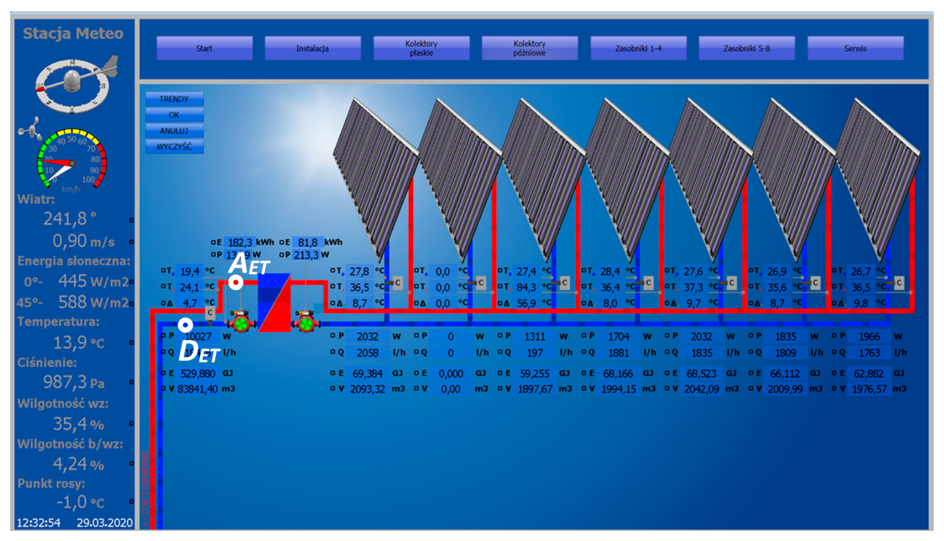
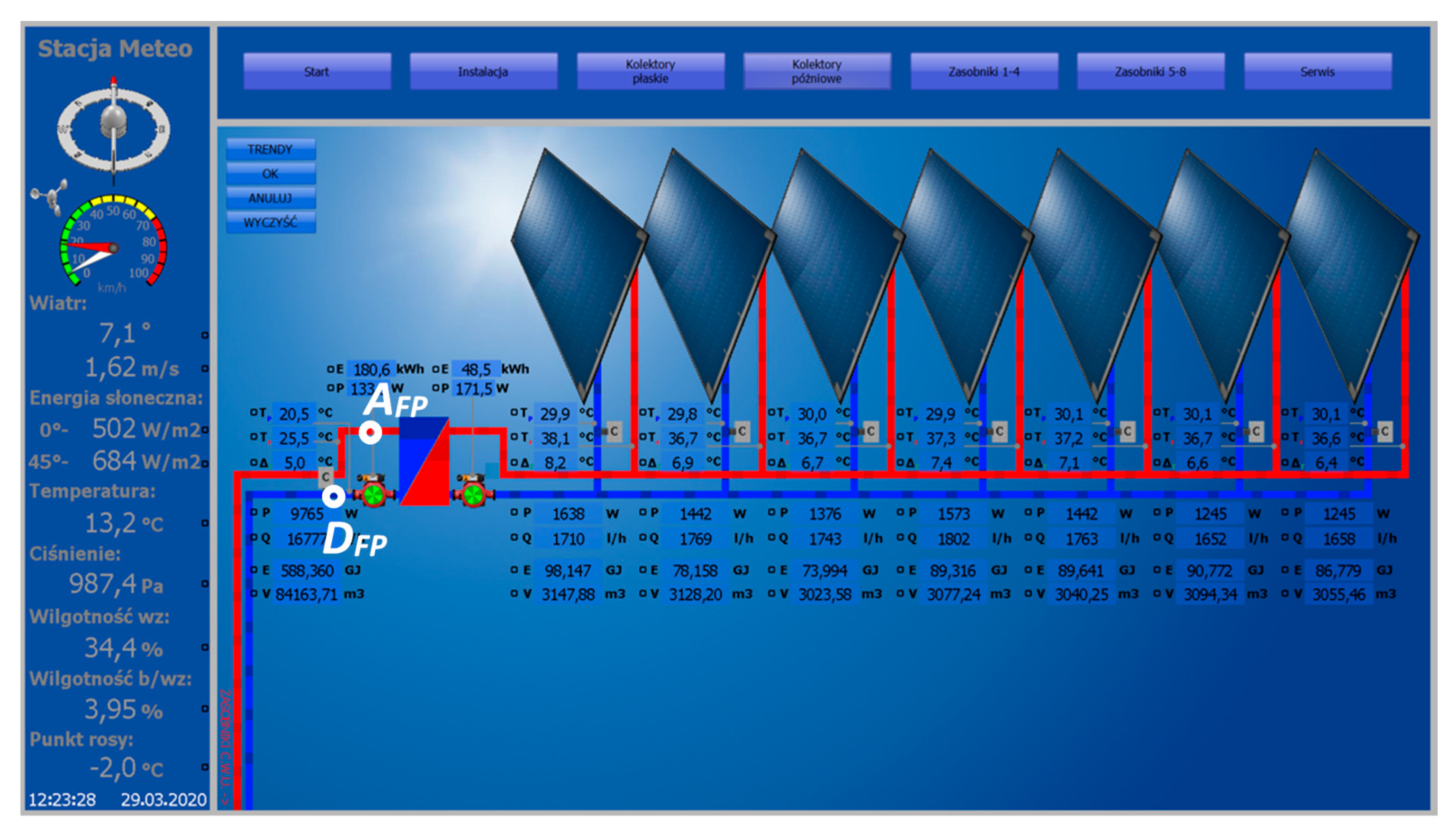
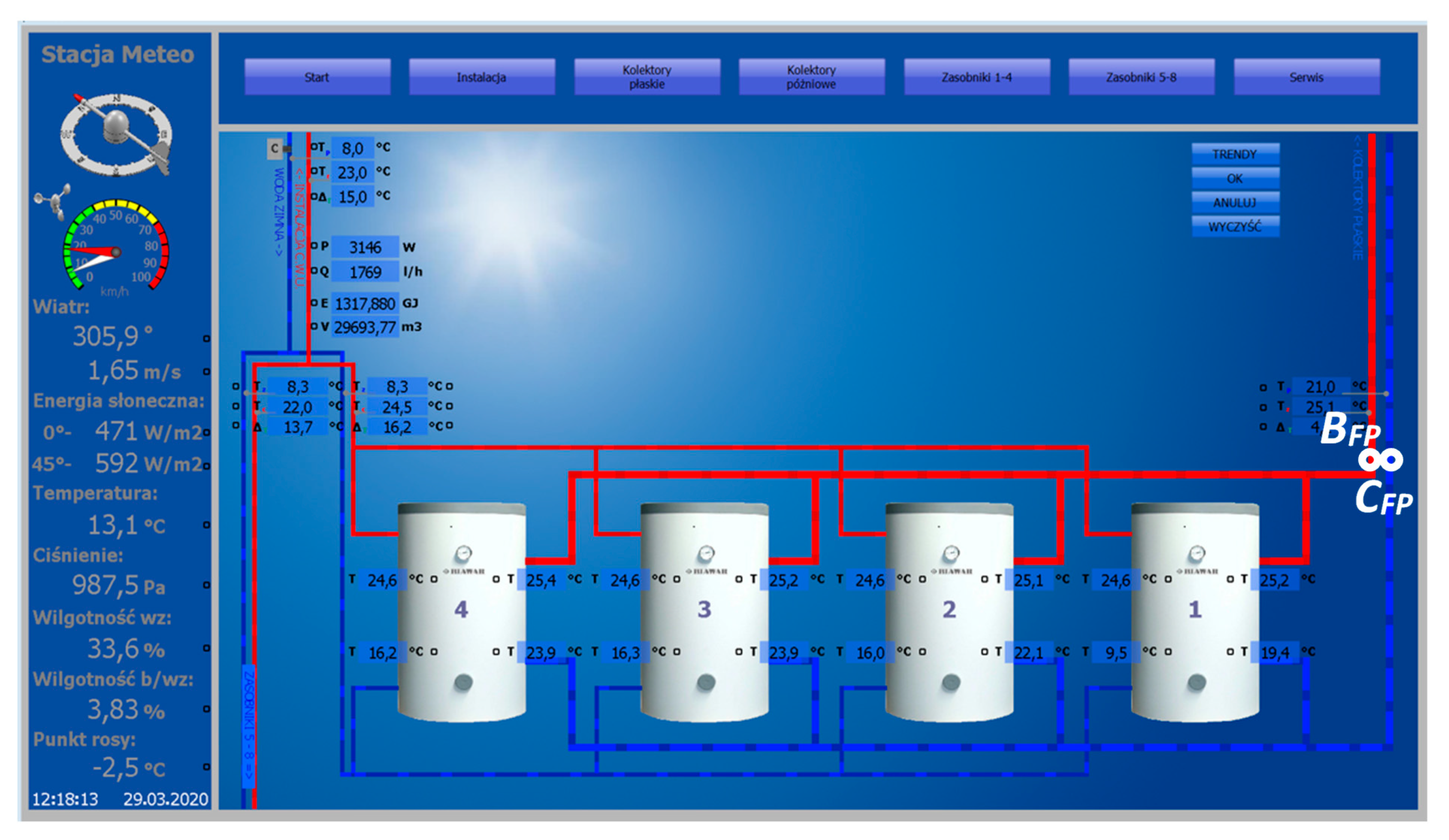
A simplified connection diagram of the system components is shown in Figure 3. The entire installation consists of two identical circuits connected in parallel.

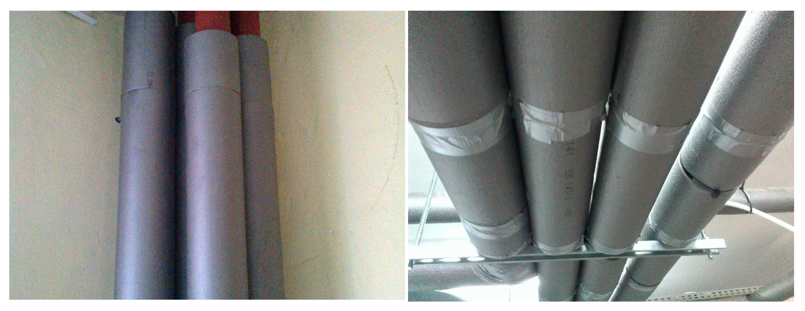
The object of this study were four pipes connecting heat exchangers located on the roof with storage tanks in the basement. They are made of light galvanized steel pipes and have a nominal diameter of DN 40. Their outer diameter is 48.3 mm and the wall thickness of 2.9 mm. The average length of each of the four pipes is 86 m. The pipelines are insulated with PE foam, which was produced by extrusion, with a thickness of 30 mm (Figure 4). The heat transfer coefficient of the insulating sleeve is equal 0.038 W/(m·K) at an average temperature of 40 °C and and its density is about 30 kg/m³.

Letters A, B mark the beginning and end of the supply pipe connecting the heat exchanger located on the roof with the storage tanks located in the basement. While the letters C and D correspond to the beginning and end of the return pipe connecting the storage tanks to the substation located on the roof. The _FP, _ET sub-indexes relate to pipes in the flat plate and evacuated tube collector loops, respectively.

3. Data Acquisition System

The operating parameters of the entire hydraulic system are monitored with a one-minute time step. The measurement results are read from 14 heat meters supporting each of the collector batteries, two heat meters measuring the energy yield of flat and evacuated tube collectors separately, and one general meter located in the heating substation. In addition, 42 Pt500 resistance temperature sensors are installed. The total temperature measurement error is approximately ±0.3 °C. In addition, four meters register electricity consumption by two solar pumps and two circulation pumps. The basic parameters of the outside air and the intensity of solar radiation are recorded by the specially dedicated weather station every 5 s. It is possible to monitor the results of measurements over the Internet. Screenshots of the monitoring system are presented in Figure 5, Figure 6, Figure 7 and Figure 8.

Selected results of temperature measurement on two supply pipelines registered at A_FP, B_FP, A_ET, B_ET points and two return pipes registered at C_FP, D_FP, C_ET, D_ET points (shown in Figure 5, Figure 6, Figure 7 and Figure 8) were used in order to determine the heat loss of the pipes.

4. Results and Discussion

4.1. Characteristics of Temperature Fluctuation in the Circulation Pipes

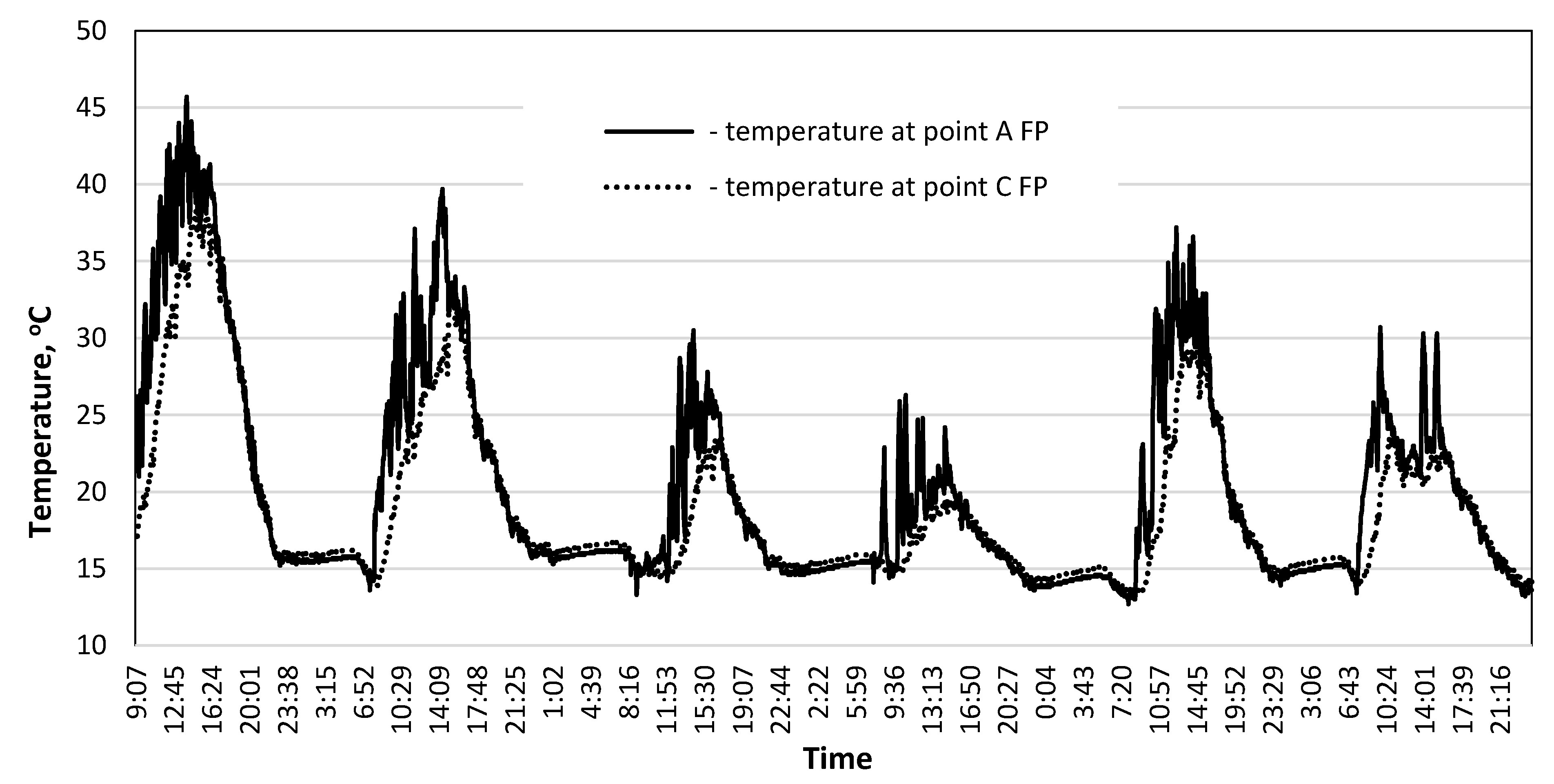
In the two analyzed loops, in which water circulates between the heat exchangers located on the roof and the heat storage tanks located in the basement, there is a continuous change in temperature. The reason for these fluctuations are, of course, changes in the amount of heat supplied by solar collectors during the day. During the night, the temperature of circulating water stabilizes. This cyclic process, illustrated in Figure 9, was shown for flat collector batteries for six days of the week. The nature of temperature variation in the vacuum collector loop was only slightly different from that shown in Figure 9, so it was not included in this article.

4.2. Determination of Heat Loss in the Classic Way

Due to the dynamic nature of the heat exchange occurring in the solar system pipes, it was decided to study this phenomenon in more detailed way. In the first stage, heat loss were determined in a classic way, i.e., using the following basic balance equations:

$$Q_S={\dot{m}}_c{c}_p\left(T_A-T_B\right) (\mathrm{for} \mathrm{supply} \mathrm{pipe}) \mathrm{and}$$

(1a)

$$Q_S={\dot{m}}_c{c}_p\left(T_C-T_D\right) (\mathrm{for} \mathrm{return} \mathrm{pipe}),$$

(1b)

where:

• ${\dot{m}}_c$—mass flow rate of water circulating in the pipes,
• c_p—specific heat at constant pressure,
• $T_A, T_C$—temperature at the beginning of the pipe (higher),
• $T_B, T_D$—temperature at the end of the pipe (lower).

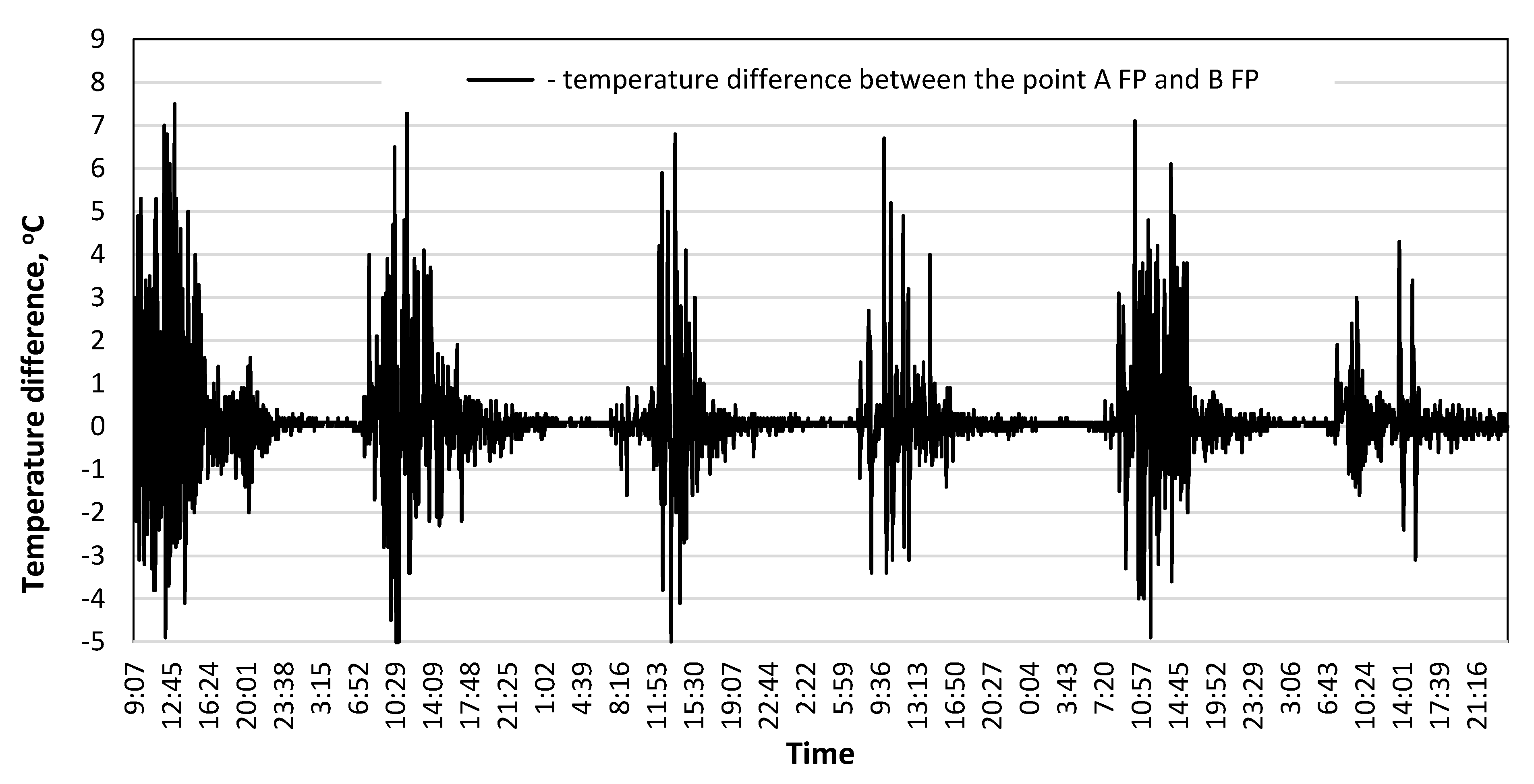
However, as the results of preliminary calculations have shown, it is not possible to use classical energy balancing equations (Equation (1)) based on determining the temperature difference at the inlet and outlet of the system. Thus, the use of heat meters to estimate energy loss will cause incorrect results, because if the return temperature is higher than the supply temperature, the measuring device will show the value 0. In fact, the heat flux is emitted from the entire surface of the pipelines.

This phenomenon results from two reasons. One is the thermal inertia of the pipes and to a lesser extent the thermal capacity of the insulation jacket. The second reason is the time of water flow through the pipeline, which was more than twice as long as the sampling time of the data recording system. The chart in Figure 10 was made to illustrate this phenomenon. The graph shows changes in temperature difference between the beginning (A_FP point) and end (B_FP point) of the supply pipe over a six-day period. As can be seen in Figure 10, there is a cyclical negative temperature difference suggesting the appearance of heat gains from the surroundings. In fact, there are still heat loss because the temperature of the water in the pipeline is higher than the temperature of the ambient air.

It was not decided to conduct experimental research involving direct measurement of heat flux density on the pipeline insulation surface due to the following reasons:

• Large error that occurs during these types of measurements (small and variable flux values).
• Large piping lengths (the need to perform measurements at large number of points simultaneously).
• Continuous temperature fluctuation inside the pipes.
• High costs of a large number of sensors and ensuring their accuracy.

Thus, a special method has been developed for estimating heat loss from pipes with variable medium temperature. This is an element of novelty, which is presented in the next part of this paper.

4.3. The New Approach to Determining the Heat Loss of Pipelines

To estimate the heat loss of pipelines with continuous fluid temperature fluctuations, a new approach has been proposed based on temperature measurements and numerical simulations. In the first step, a numerical model of the heat transfer in a pipeline was developed using algorithms of Computational Fluid Dynamics. Then this model was validated on the basis of comparison the water temperature values at the end of the pipeline as the results of calculations and measurements. A positive result of model verification ensured the correct energy balance obtained from numerical simulations. Thus, the amount of heat emitted from the outer surface of the pipeline could be determined with high accuracy based on computer calculations. As a result of this numerical analysis, two analytical equations were developed.

4.3.1. Governing Equations

The incompressible water flow inside the pipes is described by the equations of mass and energy conservation. The general form of the continuity equation (mass conservation) for 2D axisymmetric geometry is as follows [15]:

$$\frac{\partial v_r}{\partial r}+\frac{\partial v_x}{\partial x}+\frac{v_r}{r}=0,$$

(2)

where:

• ρ—fluid density,
• t—time,
• x—axial coordinate,
• r—radial coordinate,
• v_x—axial velocity,
• v_r—radial velocity.

The energy transport equation in terms of enthalpy h can be written in the following form:

$$\frac{\partial h}{\partial t}+\nabla ·\left(\overrightarrow{v}h\right)=\frac{1}{\rho }\nabla ·\left[\left(\mu +\frac{{\mu }_t}{{\sigma }_t}\right)\nabla h\right],$$

(3)

where:

• μ—viscosity,
• μ—turbulence viscosity,
• σ_t—constant.

The equations of axial and radial momentum conservation are given by [15]:

$$\frac{\partial v_r}{\partial t}+v_r\frac{\partial v_r}{\partial r}+v_x\frac{\partial v_r}{\partial x}=-\frac{1}{\rho }\frac{\partial p}{\partial r}+\frac{\mu }{\rho }\left(\frac{{\partial }^2{v}_r}{\partial r^2}+\frac{{\partial }^2{v}_r}{\partial x^2}+\frac{1}{r}\frac{\partial v_r}{\partial r}-\frac{v_r}{r^2}\right),$$

(4)

and

$$\frac{\partial v_x}{\partial t}+v_r\frac{\partial v_x}{\partial r}+v_x\frac{\partial v_x}{\partial x}=-\frac{1}{\rho }\frac{\partial p}{\partial x}+\frac{\mu }{\rho }\left(\frac{{\partial }^2{v}_x}{\partial r^2}+\frac{{\partial }^2{v}_x}{\partial x^2}+\frac{1}{r}\frac{\partial v_x}{\partial r}\right),$$

(5)

where p is a pressure.

A standard two-equation turbulence model k-ε was used for numerical simulations of transient water flow. The turbulence kinetic energy k and rate of dissipation of energy ε are presented below [15].

$$\rho \frac{\partial k}{\partial t}+\rho u_i\frac{\partial k}{\partial x_i}=\frac{\partial }{\partial x_j}\left[\left(\mu +\frac{{\mu }_t}{{\sigma }_k}\right)\frac{\partial k}{\partial x_j}\right]-\rho \epsilon +G_k,$$

(6)

and

$$\rho \frac{\partial \epsilon }{\partial t}+\rho u_i\frac{\partial \epsilon }{\partial x_i}=\frac{\partial }{\partial x_j}\left[\left(\mu +\frac{{\mu }_t}{{\sigma }_{\epsilon }}\right)\frac{\partial \epsilon }{\partial x_j}\right]+C_{1\epsilon }\frac{\epsilon }{k}{G}_k-C_{2\epsilon }\rho \frac{{\epsilon }^2}{k},$$

(7)

where, ${\mu }_t=\rho C_{\mu }\rho \frac{k^2}{\epsilon }$, G_k—generation of turbulence kinetic energy.

The default values of the constants in the above equations are equal to: C_μ = 0.09, C_1ε = 1.44, C_2e = 1.92, σ_k = 1.0, σ_ε = 1.3 [16].

4.3.2. Description of the Numerical Model

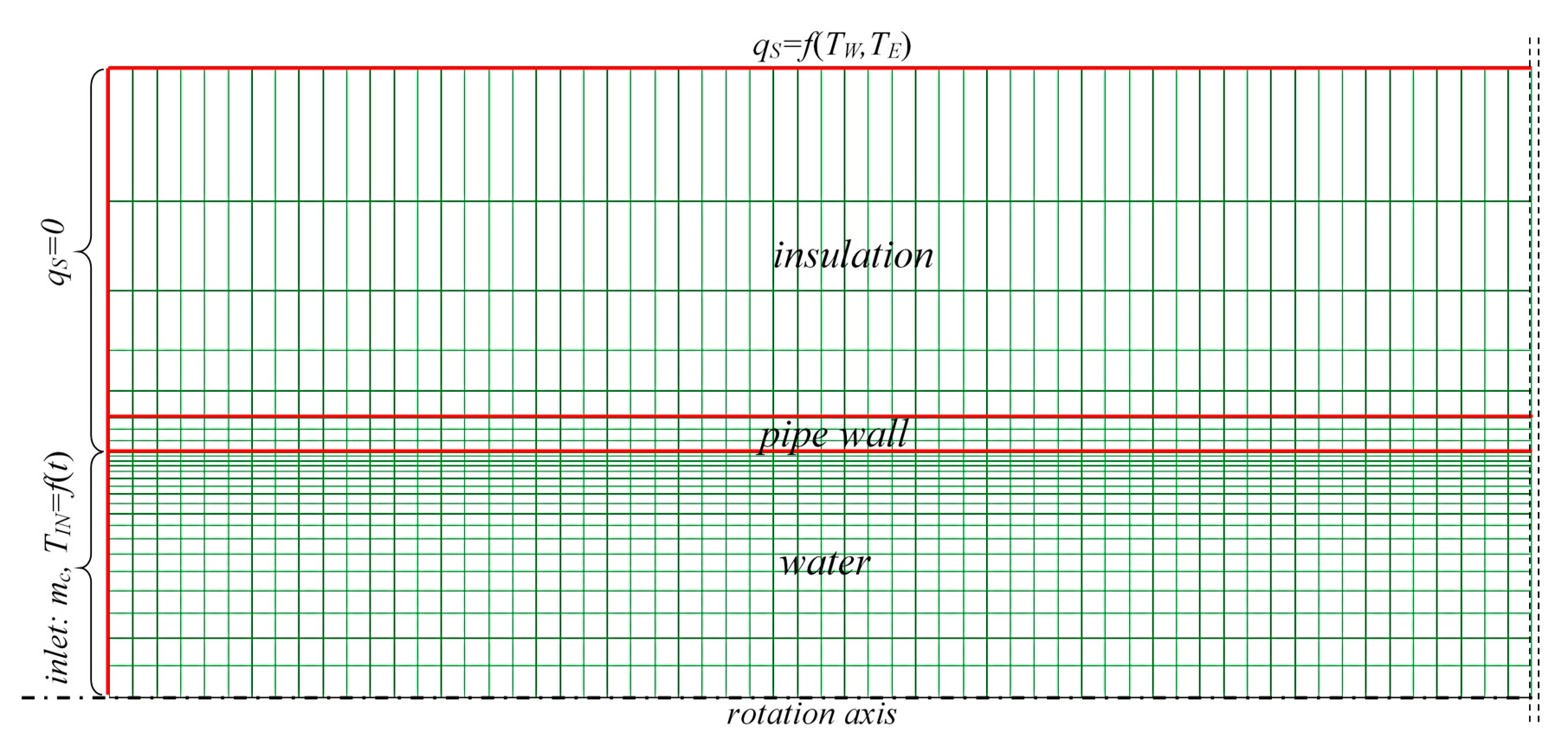
Numerical model of the pipeline with thermal insulation was developed using Ansys Release 19.2 software package. The discretization mesh, a fragment of which is shown in Figure 11, was made using a Ansys Meshing program and geometric model of the computational domain was created in the SpaceClaim program. While the calculations and processing results were carried out in Fluent solver (finite-volume numerical scheme). All these programs are integral parts of the Ansys package.

An axisymmetric geometry was applied, thanks to which this flow issue was reduced to two-dimensional. In order to select the optimal mesh density, four tests were carried out with the following number of elements: 860,000, 1,118,000, 1,419,000, 1,634,000. Area-Weighted Average Total Surface Heat Flux q_S was selected as a variable whose value was compared in each calculation series. The tests lasted 31,620 s with a time step of 60 s. The change in q_S compared to the least dense mesh was 0.311%, 0.314% and 0.316%. Therefore, for further calculations, a mesh with 1,118,000 elements and 1,147,959 nodes was used in this study. The external dimensions of the model were 86 m (length x) and 0.054 m (length y).

SIMPLE (Semi-Implicit Method for Pressure-Linked equations) algorithm for solving the pressure and velocity dependent equations was applied. The Reynolds number was higher than 20,000, therefore turbulent flow was assumed and the standard k-ε model was used, as mentioned earlier.

The equations describing the conditions at the model boundaries are shown in Figure 11. All calculations were made with a time step of 60 s.

In order to simplify the model, it was assumed that the pipeline has no bends. To increase the accuracy of calculations, the heat transfer coefficient on the outer wall of insulation was declared as a function of insulation surface temperature T_W and ambient temperature T_E. The modification of boundary conditions at the air and wall boundary using User-Defined Function (UDF) was used for this purpose. UDF was also applied to account for changes in the thermal conductivity of the insulation material depending on its temperature.

Creating an analytical model that would take into account all these assumptions described above is impossible. For this reason CFD modelling was used to determine heat loss of pipelines. This value was obtained using the Fluent postprocessor function (Reports-Surface Integrals), which enabled the generation of heat flux emitted at the external boundary of the model at each time step.

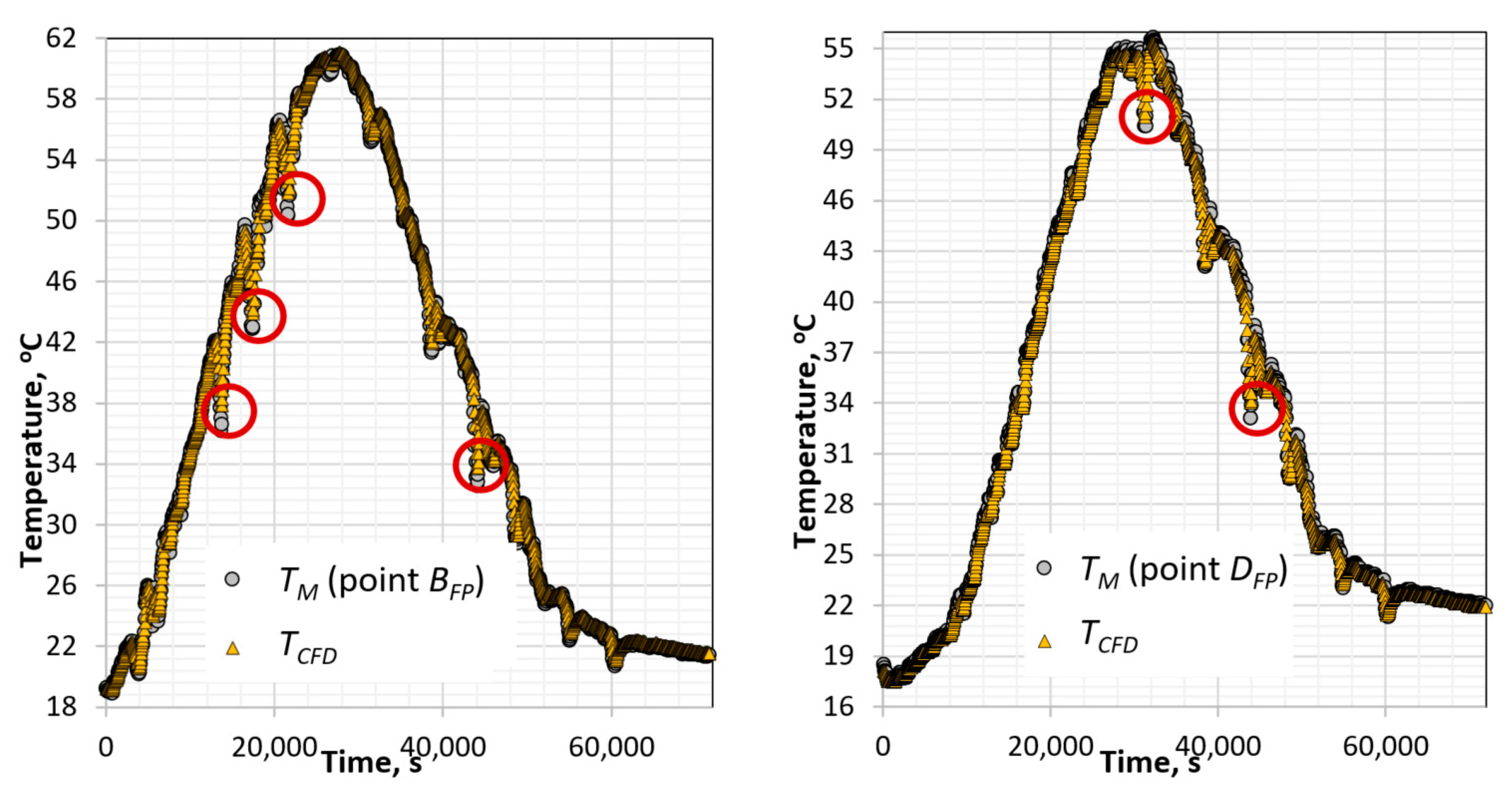
4.3.3. Validation of the Simulation Model

Verification of the accuracy of the numerical model was carried out by comparing the water temperature at the end of the pipes obtained from the measurement (T_M) and from the calculations (T_CFD). Four typical cases during the system operation were selected. The first two (P1, P2) concerned the supply (Figure 12) and return (Figure 13) pipes in the vacuum collectors loop. The next two cases (P3, P4) concerned the temperature fluctuation in the flat collector loop: the supply (Figure 14) and the return (Figure 15) pipe. The ambient temperature of pipes T_E in the analyzed measuring series was 20 ± 0.5 °C.

To determine the level of accuracy of computer simulations, two equations were used to calculate the mean relative error e_MRE (Equation (8)) and root mean square error e_RMSE (Equation (9)).

$$e_{MRE}=\frac{{{\displaystyle \sum }}_{i=1}^n\left|\frac{T_M-T_{CFD}}{T_M}\right|}{n}·100\%,$$

(8)

$$e_{RMSE}=\sqrt{\frac{{{\displaystyle \sum }}_{i=1}^n{\left(T_M-T_{CFD}\right)}^2}{k_e}},$$

(9)

where k_e = n − 1 for n < 30 and k_e = n for n > 30.

In the first two cases (P1, P2) n was 525, which corresponded to 8.75 h; and in the next two cases (P3, P4) n was equal to 1195, i.e., the simulation period was 19.9 h.

Table 1. Results of model validation.

Error	P1	P2	P3	P4
eMRE/(%)	0.91	0.24	0.82	0.53
eRMSE/(°C)	0.28	0.12	0.25	0.16

contains the results of model validation using error estimation. It turned out that the divergence between temperature values obtained from measurements and numerical calculations are quite small and are within the accuracy range of temperature sensors.

The highest differences appeared in the case of a very rapid change in temperature at the inlet to the pipe. The return temperature obtained from the calculations show that the model tends to suppress this sharp variations.

Therefore, points with maximum deviations $\left|\frac{T_M-T_{CFD}}{T_M}\right|·100\%$ were distinguished in each of these measurement series. They were marked with the red circles on Figure 12 and Figure 13. In the case of P1 (Figure 12—left graph) this difference in two points is about 10% and 8.7%; in the second case P2 (Figure 12—right graph) it is 3.9%; in the third series P3 (Figure 13—left graph) the error reaches 4.7% and in the last case P4 (Figure 13—right graph) the error value is the lowest and does not exceed 2%. However, these single cases did not affect the accuracy of modelling results in long time intervals. As can be seen, fluctuations in the supply temperature in the return pipes (P2 and P4 series) were definitely smaller compared to the changes that occurred in the supply pipes. This is due to the high thermal inertia of the storage tanks from which the return pipelines are supplied. This also translates into value of e_RMSE and e_MRE, which in the case of flow analysis in return pipes are noticeably lower.

In summary, it can be concluded that the proposed model accurately simulates the heat transfer occurring in an insulated tube and can be used to precisely determine the pipes heat loss in the second stage of this method.

4.4. Determination of the Pipelines Heat Loss

Most professional computer programs designed to simulate the buildings energy consumption and operation of HVAC systems apply meteorological databases prepared with one-hour time steps. So, it was decided to check whether assuming hourly temperature averaging, which is characterized by high variability, will affect the accuracy of the results of pipe heat loss calculations. A specific heat loss from the surface of the circulation pipes were determined using the above-described numerical model in two variants.

First, calculations were made assuming the temperature obtained from measurements T_IN (one-minute time step) as an inlet boundary condition. Then the same calculations were made using the previous input data but averaging them over one hour.

4.4.1. Determination of the Heat Loss per Unit Length of Pipe with One-Minute Time Step

Calculations of the heat flux Q_S emitted from the surface of the pipelines were made for four measurement series (P1 ÷ P4) in transient conditions. In total, 3440 values of Q_S corresponding to the supply temperature T_IN in the range from 20 °C to 60 °C were obtained. In engineering practice heat losses per 1 m of pipe length are often determined:

$$q_{S,l}=\frac{Q_s}{l},$$

(10)

where l is the length of the pipeline.

The distribution of the heat flux density q_S,l on the surface of the pipeline shows a very variable nature, which can be seen in the examples shown in Figure 14.

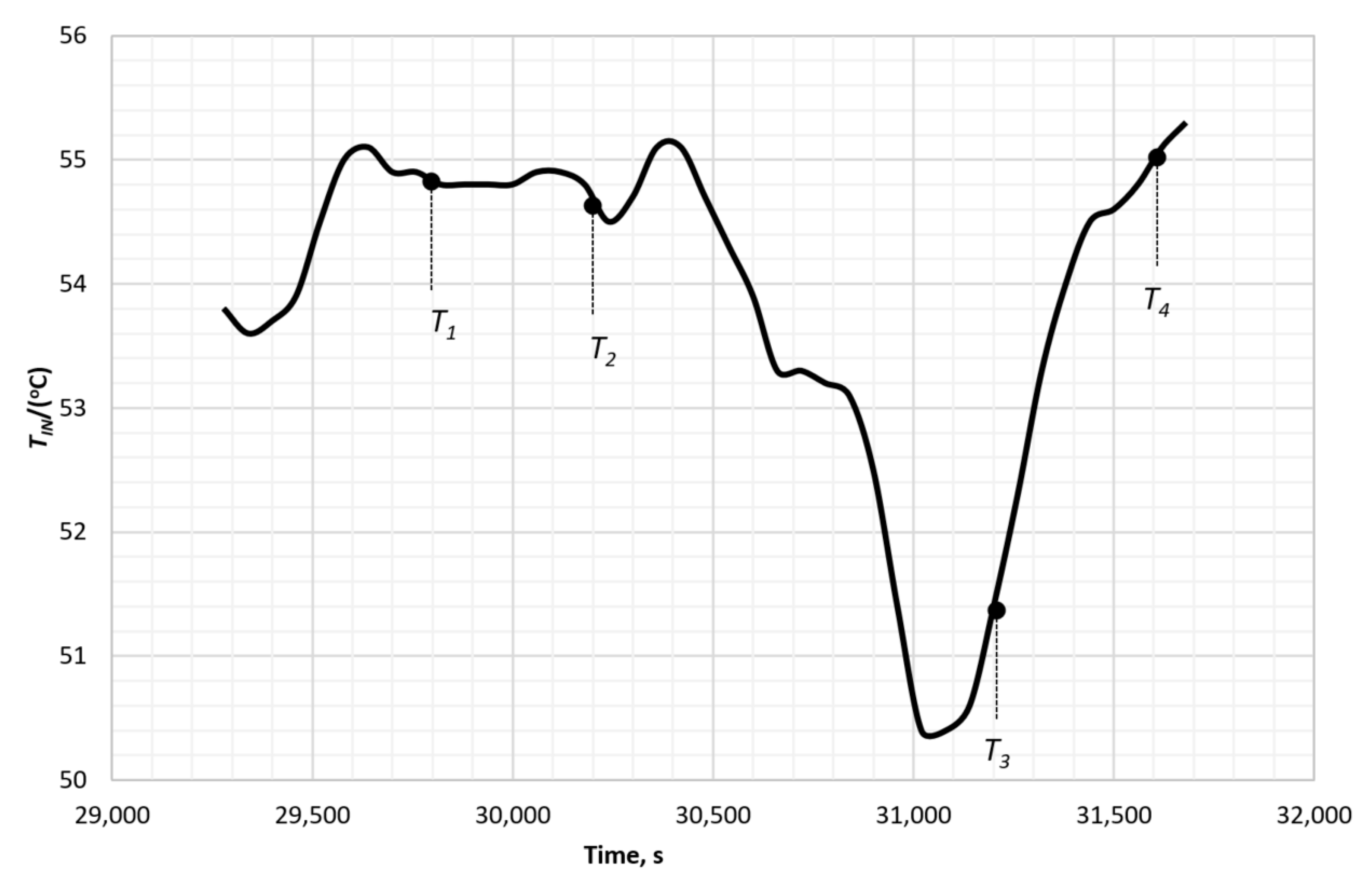
Four cases (T₁ ÷ T₄) were selected from the fragment of the inlet temperature distribution (Figure 15), for which the change in q_S,l along the pipeline length was determined. In the case of slight T_IN fluctuations, heat loss slowly decrease as a result of water cooling (T₁, T₂). A sharp change in the supply temperature (T₃) causes the reverse phenomenon, i.e., an increase q_S,l along the length of the pipe. After seven minutes of continuous increase of the inlet temperature (T₄), the tendency to change the distribution of q_S,l again reverses, showing this time the highest gradient downwards compared to the values in cases for T₁ and T₂. So, as one can see, the heat transfer on the surface of the pipeline is very dynamic and thus difficult to describe it in an analytical form.

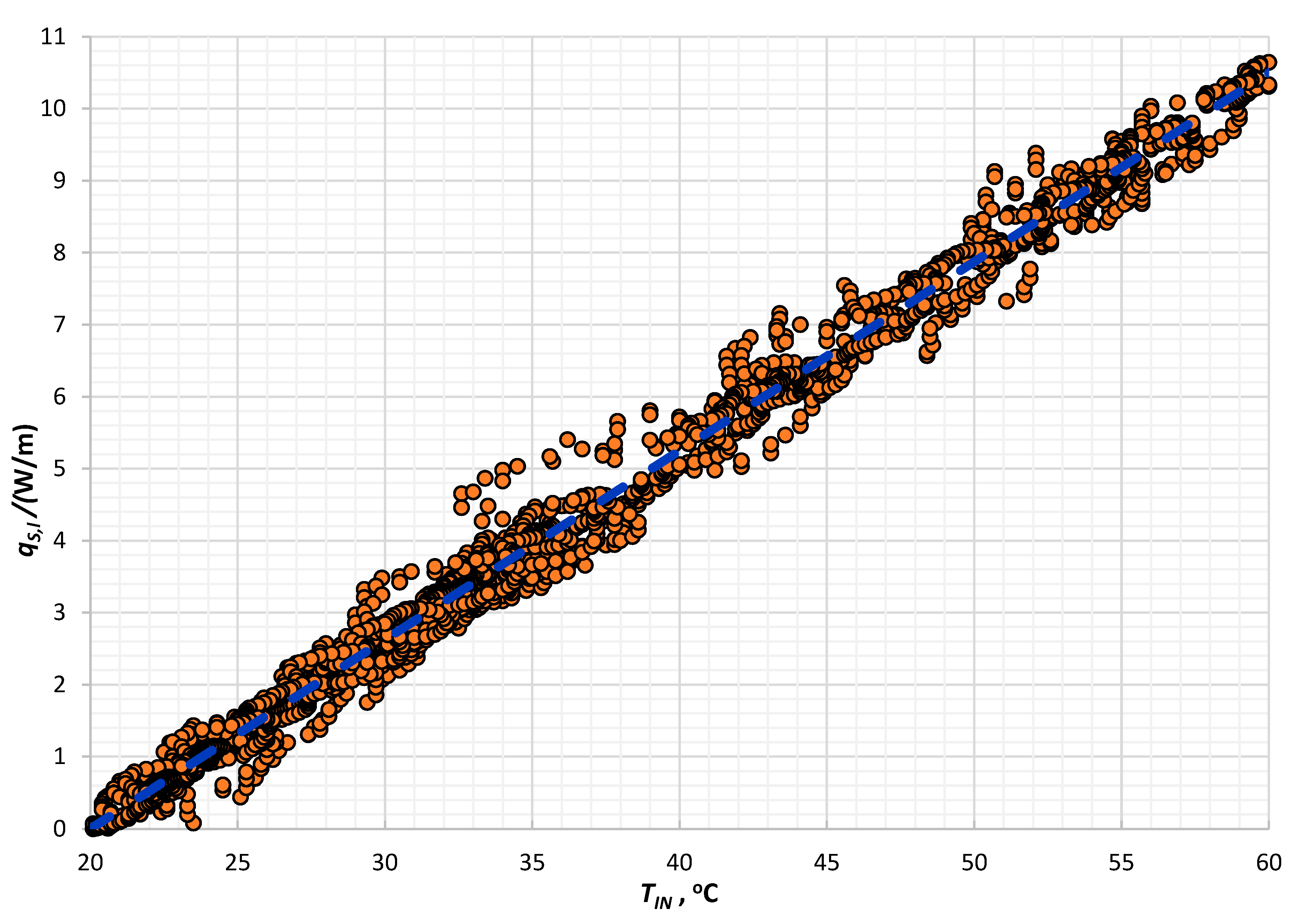
Figure 16 summarizes the results of calculations illustrating the dependence of the temperature at the inlet of the pipeline on the unit heat losses q_S,l. The dashed line indicates the trend function (Equation (11)), that approximates the results of the analysis with high accuracy, because the coefficient of determination R² is 0.9935.

$$q_{S,l}= 0.2624·T_{IN}-5.2444.$$

(11)

Equation (11) can be used to determine the heat loss of DN40 pipes protected by 30 mm-thick thermal insulation.

It is more practical in engineering applications to determine heat losses as a function of the difference in water and ambient air temperature using the following equation:

$$q_{S,l}= 0.2624·\left(T_{IN}-T_E\right).$$

(12)

If we want to calculate the amount of energy E_l lost in the Δt period, then the following relationship should be used:

$$E_l= q_{S,l}·l·\Delta t.$$

(13)

These equations can be used in the design of SDHW systems, optimization of insulation thickness and economic analyses related to the profitability of this type of installations.

4.4.2. Determination of the Heat Loss with One-Hour Time Step

As mentioned earlier, one-hour time steps are used in computer simulations due to the time-spans of meteorological parameters contained in databases. Of course, in software such as EnergyPlus or TRNSYS we can use shorter time intervals, but in this case linear interpolation of weather data is done automatically. Therefore, it was decided to calculate the heat loss of pipelines q_{S(1 h)} based on the results of the P3 and P4 measurement series, averaging inlet temperature T_IN in hourly intervals. In order to assess the accuracy of these calculations, the data presented previously obtained for a one-minute time step were averaged over an hour interval and marked q_{S(1 min)} for proper comparison both cases. Dq_S parameter was used to reflect the relative error resulting from the use of different time-spans (1 h and 1 min) and is described by the following relationship:

$$D{q}_S=\frac{q_{S\left(1min\right)}-q_{S\left(1h\right)}}{q_{S\left(1min\right)}}100\%.$$

(14)

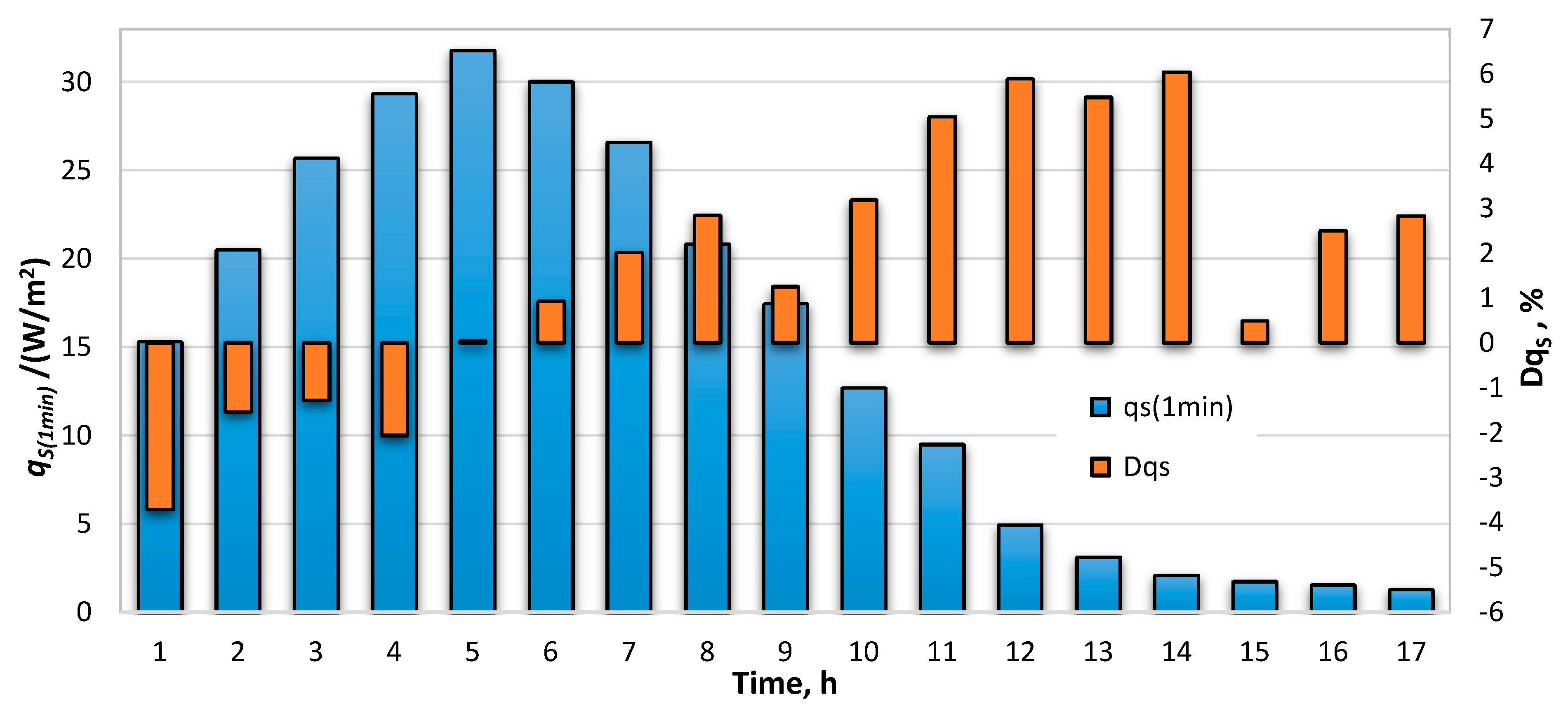
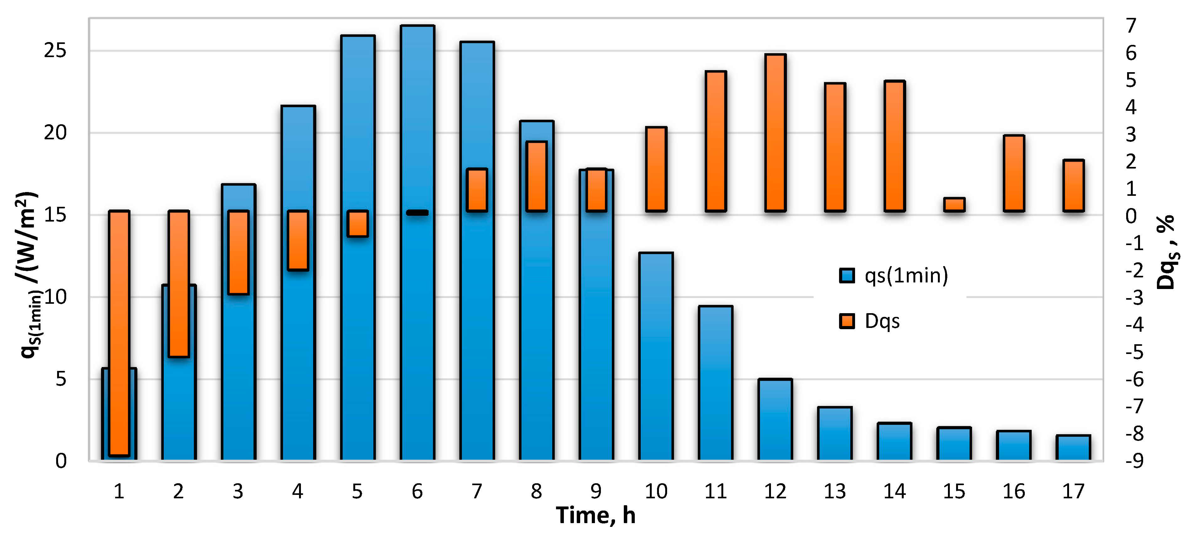
Figure 17 and Figure 18 simultaneously show the tendency to change the flux of heat loss obtained as a result of “precise” calculations q_{S(1 min)} and the parameter Dq_S for assessing the error of results obtained with a 1-h time step. Comparing these variables, two main conclusions can be drawn:

• The value of q_{S(1 h)} is overestimated in relation to “precise” calculations when heat loss tend to increase.
• We can observe reduction of q_{S(1 h)} when heat loss decreases.

However, these differences are not too high, because in the P3 series the error ranges from about −5% to over 6%, and in the P4 series from less than −9% to about 6%.

In the case of energy simulations we are interested in long periods of calculation. Therefore, the inaccuracy for the whole series of measurements was determined. For the P3 series the error was 1.8%, and in the case of second P4 series, the average error was 0.9%. This is due to the reduction of negative and positive deviations.

To sum up, it can be stated that energy simulations that are performed with a long time-spans and sinusoidal changes in heat loss trends (successive increases and decreases) will be relatively precise.

Should be noted that the issues discussed above are quite complex and do not cover the whole scope of this problem.

4.5. Determination of Nusselt Number

The Nusselt number for the flow through the pipes is calculated from the following relationship:

$$\mathrm{Nu}=\frac{h_f{D}_{in}}{k_f},$$

(15)

where, h_f—convection heat transfer coefficient, D_in—inner diameter of the pipe, k_f—thermal conductivity.

The convection heat transfer coefficient was determined based on the calculation of the heat flux q_w−f transferred through the water-pipe wall boundary:

$$h_f=\frac{q_{w-f}}{A_{w-f}·\left(T_F-T_W\right)},$$

(16)

where, A_w−f—area of heat transfer surface, T_F—water temperature, T_W—wall temperature.

The intensity of the heat transfer inside the pipe depends primarily on the Reynolds number value. Thus, the Nusselt number in the conditions occurring in the analyzed hydraulic system (Re range from 20,000 to 40,000 and average water temperature of 40 °C) can be written in the following form:

$$\mathrm{Nu}=0.037{\mathrm{Re}}^{0.8},$$

(17)

where, $\mathrm{Re}=\frac{v_f{D}_{in}}{\nu }$, v_f—average water velocity, ν—kinematic viscosity.

4.6. Pressure Loss Characteristic

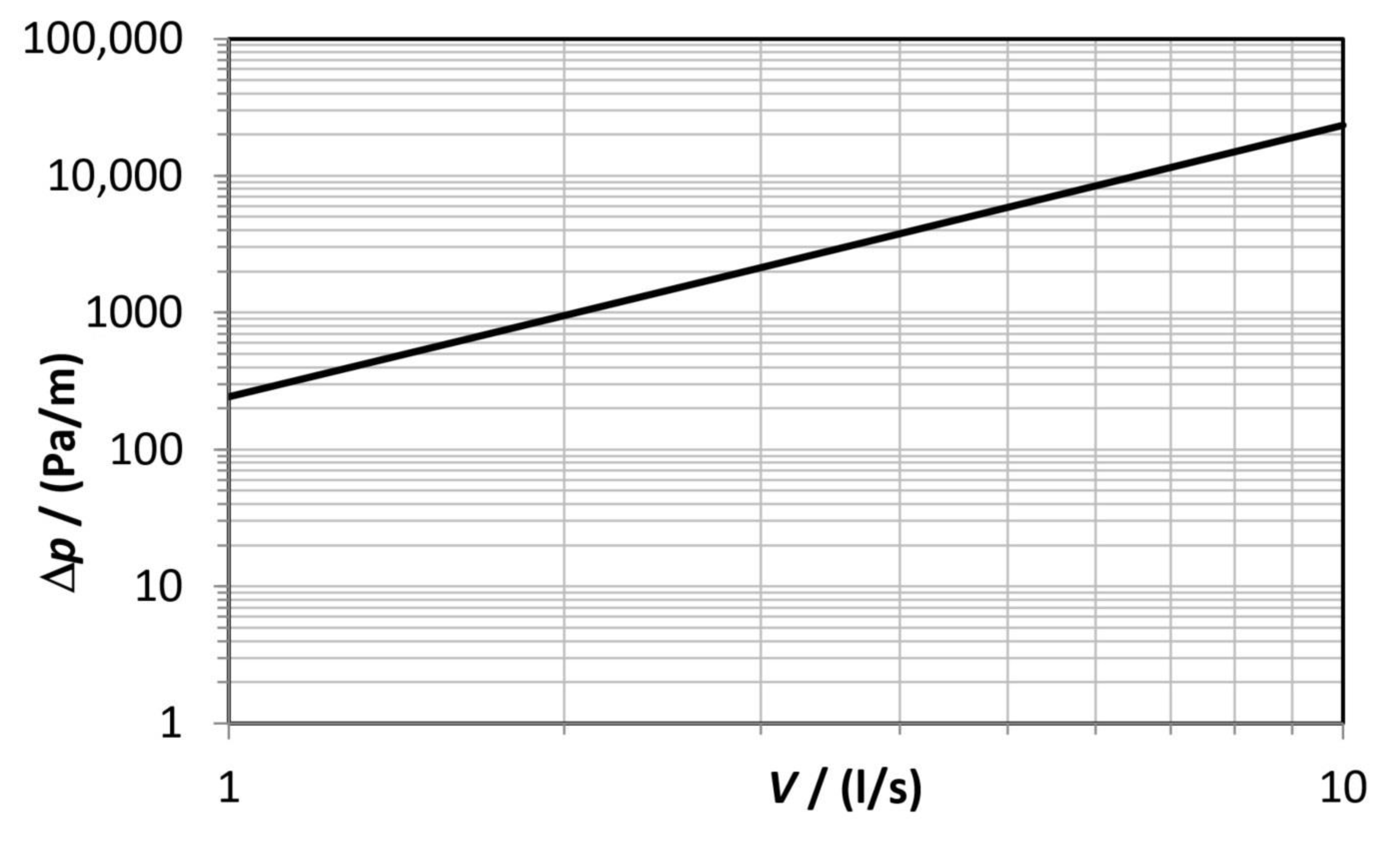
The characteristic of the pressure drop caused by the flow of water through the pipe with a nominal diameter of DN40 are shown in Figure 19.

The pressure loss related to 1 m of the pipeline length can be approximated with high accuracy (R-squared = 0.9996) by Equation (18):

$$\Delta p=242.26V^{1.9842}.$$

(18)

Thus, the pressure loss in the 86 m long pipeline DN40 section at a constant flow V = 0.63 l/s (2.28 m³/h) was 8417 Pa.

5. Summary, Conclusions, and the Future Work

The article presents the results of the analysis, which aimed to determine the heat loss of pipelines that are part of the SDHW heating system. It is supported by solar collector array consisting of 35 flat plate and 21 evacuated tube panels. Solar collectors are located on the roof of the Hotel for young researchers at Bialystok University of Technology in Bialystok (Poland). Four insulated steel pipes with a diameter of DN 40 mm and a total length of 344 m were the subject of this study. The pipelines connect heat exchangers located on the roof with heat storage tanks located in the basement of the building. There is the continuous change in the temperature circulating in these pipes due to fluctuations in the amount of energy converted by collectors during the day.

At the beginning of this work, it was decided to determine the heat loss based on measuring the flow rate and temperature difference at the inlet and outlet of the system (Equation (1)) i.e., in a classical way. However, it turned out that due to the dynamic nature of the heat exchange in the solar installation, the use of the classic energy balancing method is the cause of high inaccuracy. For this reason, a new approach has been proposed for estimating the heat loss of pipelines with a continuous change in the supply temperature. The development of a numerical model using CFD algorithms was the first step in solving this problem. Then the model was validated using the measurement results. Thus, the amount of the heat emitted from the outer surface of the pipelines in operating conditions was determined on the basis of computer calculations. The results of the supply temperature measurements taken from the data acquisition system were used as input data. Based on the approximation of a large database of computer simulation results, two relationships were proposed (Equations (11) and (12)). They are the practical result of this work and can be used in engineering calculations. It allows estimating the heat loss of pipelines in stationary heat exchange conditions as a function of the difference in water and ambient air temperature.

Building energy simulation software usually uses meteorological databases prepared with an one-hour time step. It was also decided to estimate the error resulting from assuming hourly averaging of SDHW system operation parameters. Based on a comparison of the results of the heat loss calculations carried out with a 1-h and 1-min step, it can be concluded that the differences for these time-spans are quite large and range from −9% to 6%. However, when it was balanced the whole day of the system operation, the total error did not exceed 2% due to the elimination of divergences between the first and second half of the measurement series.

In the next stage of this work, it is planned to develop the universal equations that will allow the calculation of heat losses from pipes of different diameters and different thickness and types of thermal insulation materials.