Downward Annular Flow of Air–Oil–Water Mixture in a Vertical Pipe

Abstract

The paper presents the results of a study concerned with the hydrodynamics of an annular downward multiphase flow of gas and two mutually non-mixing liquids through a vertical pipe with a diameter of 12.5 mm. The air, oil and water were used as working media in this study with changes in superficial velocities in the ranges of j_g = 0.34–52.5 m/s for air, j_o = 0.000165–0.75 m/s for oil, and j_w = 0.02–2.5 m/s for water, respectively. The oil density and viscosity were varied within the ranges of ρ_o = 859–881 kg/m³ and η_o = 29–2190 mPas, respectively. The research involved the identification of multiphase flow patterns and determination of the void fraction of the individual phases. New flow patterns have been identified and described for the gravitational flow conditions of a two-phase water–oil liquid and a three-phase air–water–oil flow. New flow regime maps and equations for the calculation of air, oil and water void fractions have been developed. A good conformity between the calculated and measured values of void fraction were obtained. The map for the oil–water–air three-phase flow is valid for the following conditions: j_3P = 0.35–53.4 m/s (velocity of three-phase mixture) and oil in liquid concentration β_o* = 0.48–94% (oil in liquid concentration). In the case of a downward annular oil–water two-phase flow, this map is valid for liquid mixture velocity j_l = 0.052–2.14 m/s and β_o* = 0.48–94%.

1. Introduction

The co-current flow of a mixture comprising two non-mixing liquids and gas occurs in a variety of apparatus in the chemical and food industries, as well as in the petrochemical and plastics branches. The industrial use of multiphase flows involves the need to develop computational methods capable of predicting their behaviors in specific types of equipment and apparatus. In many cases, for the purpose of the adequate operation of the apparatus, it is also necessary to generate a desired type of flow. Thin-film evaporators or tubular heterogeneous reactors can be listed in this category (Cyklis [1], Czernek et al. [2] and Nagavarapu et al. [3]). Among this class of apparatus, the preferred conditions include annular flow, i.e., one in which the liquid flow occurs in the form of a thin film along the pipe wall accompanied by gas flow with a considerable velocity through its center. In the processes of the design of apparatus using the annular flow of a multiphase mixture, problems are faced in relation to determining such quantities as ranges of occurrence of various flow patterns, the actual values of void fractions of the phases, and the values of the thickness of the liquid films that play significant roles in the pipes of the thin-film apparatus. It is also very important to take into account the fact that one of the phases of the two-phase liquid needs to be taken to be the continuous phase and the other as the dispersed phase. This has a direct effect on the efficiency of the heat and mass transfer processes, which is indicated by, among others, studies by Witczak et al. [4], Czernek et al. [5], Dong et al. [6], Hamidi et al. [7] and Guichet et al. [8].

Nowadays, two-phase gas–liquid flows have been well explored and reported in the literature, as have three-phase gas–liquid–liquid mixtures in horizontal channels, but despite the significant practical importance much fewer studies focus on the hydrodynamics of three-phase gas–liquid–liquid flows through vertical channels, and especially on the downflow of mixtures with very viscous liquids.

The majority of the published works in this field emphasize the very complex nature of the hydrodynamic phenomena accompanying such flows, and the adequate interpretation of them still forms a challenge for scientists and practicing engineers. These flows are accompanied by specific phenomena, such as an effect of reducing pressure drops, phase inversion, interfacial slip, as well as the formation of liquid emulsions in the mixture. Extensive numerical and experimental studies were described in Sobolewski et al. [9], Edwards et al. [10], Edwards et al. [11] and Edwards et al. [12]. The knowledge of listed characteristic phenomena in a three-phase flow becomes particularly important when the designed apparatus and installations will be operated in these specific conditions.

The scope and basic information of the research works carried out so far for vertical three-phase flow are summarized in Table 1.

Poettmann et al. [13] and Tek [14] conducted the first studies on the three-phase flow of natural gas, water and oil in pipes of vertical wells. On the basis of experimental data, the authors developed correlations for calculating pressure drops in vertical pipes. In turn, Foreman et al. [15] developed a two-phase flow slip model for calculating the gas void fraction in a three-phase mixture.

Shean [16] and Pleshko et al. [17] conducted an analysis of the possibility of using two-phase models to determine the transition boundaries between individual three-phase patterns. Furthermore, they calculated the gas void fractions and pressure drops in the three-phase flow.

The three-phase flows of gas and two non-mixing liquids are explored more comprehensively by Woods et al. [18], Spedding et al. [19], Oddie [20], Shi et al. [21], Descamps et al. [22,23], Nowak [24] and Nowak et al. [25]. In these works, the authors gave, among other things, detailed classifications of three-phase patterns, and attempted to describe changes in total pressure drops, taking into account the value of the volume fraction of particular phases.

The latest works on this subject include studies reported by Pietrzak et al. [26] and Colmanetti et al. [27]. The authors attempted to determine the influences of gas velocity and liquid viscosity on the course of the phenomena accompanying phase inversion in the water–oil system during three-phase mixture flow, and the effect of this phenomenon on the pressure drop. We can also note the areas explored in studies by Wang et al. [28] and Bannwart et al. [29]. The authors investigated the conditions of three-phase co-current flow in both horizontal and vertical channels, pointing to significant similarities and differences in the phenomena accompanying these flows. In these studies, the authors applied high-viscosity oils (0.15–3.4) Pas. This research demonstrated the significant effect of oil viscosity on the hydrodynamics of liquid phase flow.

Three-phase flow in hilly terrain pipelines with different inclinations was investigated by Huang et al. [30]. The results demonstrated that different structures are formed in the case of the air–oil–water upflow and downflow in pipelines with a diameter of 40 mm inclined at an angle of 30°. They noticed significant changes in pressure drop values accompanying changes in flow patterns during the flow of the multiphase mixture. The influence of flow direction on the three-phase flow patterns was also the subject of research conducted by Hanafizadeh et al. [31]. The authors of Ref. [31] conducted research on the three-phase flow in a pipe with an internal diameter of 20 mm and an angle of inclination ±45° in relation to the horizontal. In both cases, the test results confirmed the significant effects of the physicochemical properties of the phases and their velocity on the hydrodynamics of three-phase flow both for upflow and downflow.

The influence of the flow direction of the three-phase mixture, both for upflow and downflow, on the formation of flow patterns was investigated by Brandt [32]. In this study, the measurement techniques applied in the study of multiphase flow hydrodynamics were also described. In turn, Goshika et al. [33] investigated the problems of feeding a column operating with a falling three-phase gas–liquid–liquid flow. They studied the effect of the supply system (contactor) on the hydrodynamics of a falling air–kerosene–oil three-phase flow at different operating conditions. They developed models to assess liquid entrainment and holdup in the column for this type of three-phase mixture.

An analysis of the work on the three-phase flow in vertical pipes shows that most of the experimental studies were conducted for the upward flow of the mixture. Only a few of the papers (Huang et al. [30], Hanafizadeh et al. [31], Brandt [32] and Goshika et al. [33]) discuss issues related to research on downward flow in vertical and inclined pipes. Based on the current state of the art, it is difficult to generalize the description of the complex phenomena occurring during such a flow.

Table 1. Summary of research into the hydrodynamics of upward three-phase gas–liquid–liquid flow in vertical pipes.

No.	Author	Mixture Components	Channel Diameter	Oil Properties		Scope of Experiment
				Density	Viscosity
			mm	kg/m3	mPas
1	Poettmann et al. [13] (1952)	paraffin–water–air	boreholes	-	-	pressure drop
2	Tek [14] (1961)	paraffin–water–air	borehole	-	-	pressure drop, void fraction
3	Foreman [15] (1975)	paraffin–water–air	19	810	1.5	void fraction
4	Shean [16] (1976)	oil–water–air	19	889	71.8	flow patterns, void fraction, pressure drop
5	Pleshko et al. [17] (1990)	oil–water–air	51	814	7.48	flow patterns, gas void fraction, frictional pressure drops
6	Woods et al. [18] (1998)	oil–water–air	26	829	12	flow patterns, void fraction, pressure drop
7	Spedding et al. [19] (2000)	oil–water–air	26	829	11	flow patterns, void fraction, pressure drop
8	Oddie et al. [20] (2003)	paraffin–water–nitrogen	152	810	1.5	flow patterns, void fraction
9	Huang et al. [30] (2003)	oil–water–air	40	870	117	flow patterns for pipe inclination of −30° (upward and downward)
10	Shi et al. [21] (2004)	paraffin–water–nitrogen	15	810	1.5	void fraction
11	Descamps et al. [22] (2006)	oil–water–air	82.8	830	7.5	effect of gas injection on critical concentration of oil and water at phase inversion point, pressure drop
12	Nowak [24] (2007)	oil–water–air	30	860	20	flow patterns, void fraction, pressure drop
13	Bannwart et al. [29] (2009)	oil–water–air	28.4	970	3.4	flow patterns, pressure drop
14	Wang et al. [28] (2012)	oil–water–natural gas	52.5	-	150–570	flow patterns, gas void fraction, frictional pressure drop
15	Brandt [32] (2015)	oil–water–air	12.5	860–880	16–2000	flow patterns, void fraction, liquid film thickness
16	Pietrzak et al. [26] (2017)	oil–water–air	30	856	29	flow patterns, void fraction of phases, pressure drop
17	Hanafizadeh et al. [31] (2017)	oil–water–air	20	840	4.5	flow patterns for pipe inclination of −45° to +45° (upward and downward)
18	Colmanetti et al. [27] (2018)	oil–water–air	50, 95	900	70–280	flow patterns, pressure drop

Table 1. Summary of research into the hydrodynamics of upward three-phase gas–liquid–liquid flow in vertical pipes.

No.	Author	Mixture Components	Channel Diameter	Oil Properties		Scope of Experiment
				Density	Viscosity
			mm	kg/m3	mPas
1	Poettmann et al. [13] (1952)	paraffin–water–air	boreholes	-	-	pressure drop
2	Tek [14] (1961)	paraffin–water–air	borehole	-	-	pressure drop, void fraction
3	Foreman [15] (1975)	paraffin–water–air	19	810	1.5	void fraction
4	Shean [16] (1976)	oil–water–air	19	889	71.8	flow patterns, void fraction, pressure drop
5	Pleshko et al. [17] (1990)	oil–water–air	51	814	7.48	flow patterns, gas void fraction, frictional pressure drops
6	Woods et al. [18] (1998)	oil–water–air	26	829	12	flow patterns, void fraction, pressure drop
7	Spedding et al. [19] (2000)	oil–water–air	26	829	11	flow patterns, void fraction, pressure drop
8	Oddie et al. [20] (2003)	paraffin–water–nitrogen	152	810	1.5	flow patterns, void fraction
9	Huang et al. [30] (2003)	oil–water–air	40	870	117	flow patterns for pipe inclination of −30° (upward and downward)
10	Shi et al. [21] (2004)	paraffin–water–nitrogen	15	810	1.5	void fraction
11	Descamps et al. [22] (2006)	oil–water–air	82.8	830	7.5	effect of gas injection on critical concentration of oil and water at phase inversion point, pressure drop
12	Nowak [24] (2007)	oil–water–air	30	860	20	flow patterns, void fraction, pressure drop
13	Bannwart et al. [29] (2009)	oil–water–air	28.4	970	3.4	flow patterns, pressure drop
14	Wang et al. [28] (2012)	oil–water–natural gas	52.5	-	150–570	flow patterns, gas void fraction, frictional pressure drop
15	Brandt [32] (2015)	oil–water–air	12.5	860–880	16–2000	flow patterns, void fraction, liquid film thickness
16	Pietrzak et al. [26] (2017)	oil–water–air	30	856	29	flow patterns, void fraction of phases, pressure drop
17	Hanafizadeh et al. [31] (2017)	oil–water–air	20	840	4.5	flow patterns for pipe inclination of −45° to +45° (upward and downward)
18	Colmanetti et al. [27] (2018)	oil–water–air	50, 95	900	70–280	flow patterns, pressure drop

Considering the above, the main objective of the work is to complete and extend the knowledge in the field of the hydrodynamics of co-current air–water–oil three-phase downflow through vertical pipes, with particular emphasis on liquids with high viscosity. The determination of the flow conditions at which the particular flow patterns occur, as well as the description of how the flow parameters and properties of the mixture components influence the values of the void fraction in the multiphase mixture, are explored.

2. Materials and Methods

Scope of Experiment

The experimental tests involving air–oil–water three-phase flow were carried out in an experimental stand presented in Figure 1.

The measurement of the temperatures of individual fluids (in the range of 15 to 30 °C) was carried out using a K-type thermocouple system with an accuracy of T_i ± 0.1 K. The oil was fed from the tank (1) to the installation and supply system (with a central nozzle) by means of a gear pump (2), driven by a DC motor, which ensured smooth regulation of the pump rotating speeds. Four types of oils were used in the tests: LAN-15 machine oil, and three types of Itherm oils (6, 12 and 30 MF) with different densities and viscosities found in the ranges of ρ_o = 850–881 kg/m³ and η_o = 29–2190 mPas, respectively. Water was extracted directly from the water supply network (ρ_w = 990–1000 kg/m³ and η_w = 0.95–1.1 mPas), pumped to the water tank (18) from where after degassing by means of a hydrophore (19) it was routed to the channel supply system, through a battery of water flowmeters. The air was extracted from the central compressed pressure system (0.6 MPa) and after passing through the reducing valve (12), it was directed to the flowmeter battery (11), where its flow rate was controlled and measured. The measurements of air temperature and pressure (using K-type thermocouples and Peltron pressure transducers, respectively) indicated ρ_g = 1.15–1.25 kg/m³ and η_g = 0.018 mPas.

The multiphase mixture produced in a mixing chamber (K) initially flowed through the opaque section of the test channel (10) where the flow stabilized and flow patterns formed. In the transparent part of the measuring channel (3), the observation and identification of flow patterns were performed, combined with measurements of the void fraction of the phases conducted using the trap method (5, 6, 7). A system of electrical conductivity probes (15) was used for the determination of the dominance of oil or water phase in the flow. Output signals from the probes used to determine the presence of individual liquid phases on the walls of the measuring channel were recorded using a 16-channel NI USB-6210 analog-digital measuring card from National Instruments (16), which was offered by the recorded DC voltage signals in the range of 0 to 5 V with an accuracy of ±1.0 mV.

The actual characteristics of the voltage variations for two-phase liquid–liquid flow are presented in Figure 2. These characteristics correspond to the following flows: water dominated flow—O/W, oil dominated flow—W/O and emulsified flow—(O + W), in which latter case it was unfeasible to clearly determine which of the liquid phases was dominant in the flow. The mean voltage values characteristic of a given type of flow are also marked on the waveforms of the provided voltage characteristics.

Flow patterns were recorded with a Canon EOS 300D digital camera and video camera. The camera used to take pictures of the flow structures had a shutter speed of 1/4000s, and the video camera recorded movies at a resolution of 1024 × 1024 pixels with a frequency of 1800 Hz.

After the three-phase mixture had passed through the measuring channel, it was routed into the pre-separator (13), in which gas and liquid were separated. Then, using a Grundfos centrifugal pump, the liquid mixture separated from the air was pumped into the final separator (21) with a capacity of 1000 dm³, where the mixture components were separated into oil and water by gravity. The measuring instruments were connected to the computer-based data acquisition system (17).

The experiments were carried out with a wide range of variations in flow parameters and properties of fluids. The range of the flow parameter changes for the three-phase air–water–oil mixture and the characteristics of oils at 20 °C are presented in

Table 2. The range of parameters change in multiphase mixture flow.

Mixture Component	Flow Rate	Superficial Velocity		Reynolds Number		Inlet Void Fraction
	Qi, m3/h	ji, m/s		Rei, -		βi, -
Air	0.15–23.2	0.34–52.5		271–43,870		0.1–0.99
Water	0.007–1.1	0.02–2.5		181–32,632		0.095–0.98
L-AN 15 oil	0.012–0.33	0.028–0.75		11–300		0.027–0.94
Iterm 6 Mb oil *	0.00096–0.33	0.0022–0.75		0.3–110		0.024–0.9
Iterm 12 oil	0.001–0.17	0.0028–0.22		0.12–20		0.0086–0.94
Iterm 30MF oil	7.31 × 10−5–0.022	0.000165–0.05		0.0007–12		0.0017–0.7
Physical Properties of Oils at Temperature of 20 °C
Oil	Density, kg/m3		Viscosity, mPas		Surface Tension, mN/m
L-AN 15	859.8		29		32.47
Iterm 6 Mb	860.7		83		35.85
Iterm 12	881.5		37		61.43
Iterm 30 MF	880.8		2190		91.23

* The tests were carried out only for the gravitational downflow of a two-phase liquid–liquid mixture, due to the significant emulsification of the system at higher multiphase flow velocities.

.

The values of the Reynolds number for individual phases, Re_i, (Table 2) and the values of the volume ratios of the phases at the inlet to the pipe (ratios of phase flow rate), β_i, were determined as:

$${Re}_i=\frac{j_{i}d{\rho }_i}{{\eta }_i}$$

(1)

$${\beta }_i=\frac{j_i}{j_g+j_w+j_o}=\frac{j_i}{j_{3P}}$$

(2)

The superficial velocity (which by definition is calculated per entire pipe cross-section) was derived from the following relation:

$$j_i=\frac{4Q_i}{\pi d^2},$$

(3)

where Q_i is the volume flow rate of the i-th phase, m³/s, and d is the internal diameter of the pipe, m. The tests were carried out for ten constant values of air flow rates, as well as eight and thirteen constant values of the flow rates of oils and water of different characteristics, respectively. Each measurement lasted for the duration of 10–90 s (depending on the physical properties of the oils applied in the tests).

3. Results and Discussion

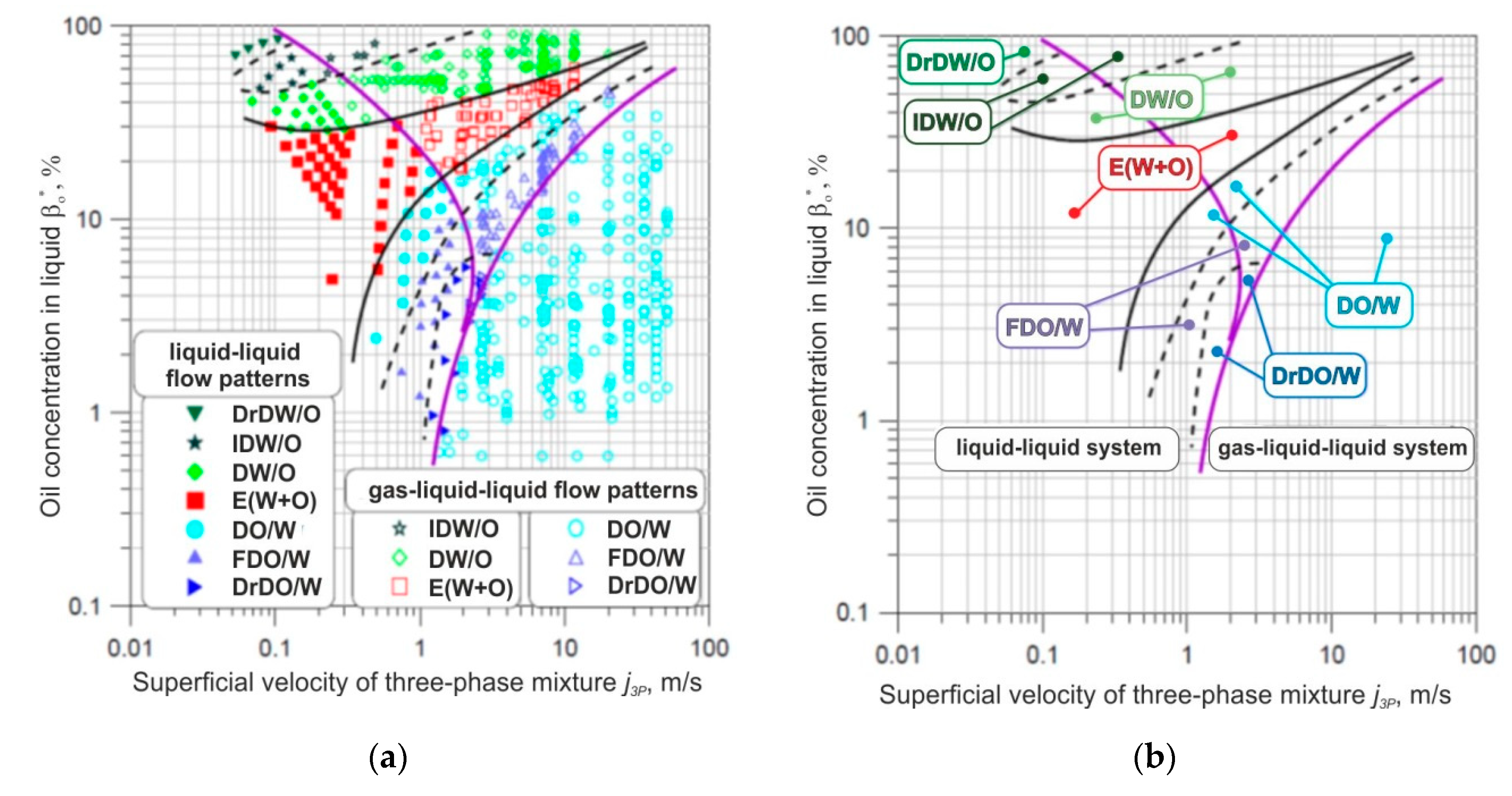
3.1. Flow Patterns

Three-membered abbreviation was applied to define the identified multiphase flow patterns. The first part of the name describes the nature of the phase distribution in the gas–liquid system (e.g., A—annular pattern), the second part refers to the flow patterns of the dispersed liquid (e.g., D—dispersion of a given liquid component). The third part of the name indicates the type of dispersed and continuous component that dominates in the flow (e.g., O/W—oil in water). Taking into account all the observed and registered forms of flow and the results of conductometric tests obtained for them, they were classified according to the proposed scheme.

During tests of water–oil downflow two-phase flow through a vertical channel, seven basic flow patterns were identified: three patterns characterized by water-dominated flow (DrDO/W—drops of dispersed oil in water continuum, FDO/W—bubble-dispersed oil in water continuum, DO/W—dispersed oil in water continuum), three patterns with oil-dominated flow (DrDW/O—drops of dispersed water in oil continuum, IDW/O—intermittent dispersed water flow in oil continuum, DW/O—dispersed water flow in continuous oil phase) and one transient pattern with properties of emulsion, which was classified as intermittent flow E (W + O).

In a similar manner to the case of two-phase liquid–liquid flow, the patterns accompanying the downflow of three-phase air–water–oil mixture in the vertical pipe were also identified and described. The names and letter abbreviations were assigned to all observed flow structures. Due to the similarity of the characteristics of both of these flows, a prefix with the symbol “A” was added to the names employed to refer to the two-phase water–oil flow, in the case of three-phase flow, indicating the annular characteristics of the flow. In this way, for the flow with the dominant water phase, the following patterns were distinguished: annular with drops of dispersed oil in water—A-DrDO/W; annular with dispersed foam of oil in water—A-FDO/W; annular with dispersed oil in water—A-DO/W. In turn, for the oil-dominated flow, the following patterns were distinguished: annular with dispersed drops of water in oil—A-DrDW/O; annular with intermittent-dispersed water in oil—A-IDW/O and annular with water dispersion in oil—A-DW/O. It should be emphasized that along with the decay of the gas phase flow, these patterns correspond to the ones recorded for the gravitational flow of two non-mixing liquids.

Table 3. Air–water–oil three-phase downflow patterns in vertical pipe for η_o = 0.159 Pas.

Water Dominated Flow (O/W)			Emulsified Flow (O + W)	Oil Dominated Flow (W/O)
A-DrDO/W	A-FDO/W	A-DO/W	A-E(W+O)	A-IDW/O	A-DW/O	DrDW/O
jg = 2.485	3.457	11.32	2.485	3.887	8.432	0.982 m/s
jw = 0.141	0.742	0.742	0.230	0.110	0.110	0.186 m/s
jo = 0.036	0.120	0.094	0.210	0.158	0.158	0.210 m/s

presents images of the three-phase air–water–oil flow patterns derived for the case in which various velocities of individual phases were applied in the experiment. In turn,

Table 4. Schematic diagrams of gas–liquid–liquid downflow patterns in vertical pipes.

Water Dominated Flow (O/W)			Emulsified Flow (O + W)	Oil Dominated Flow (W/O)
A-DrDO/W	A-FDO/W	A-DO/W	A-E(W+O)	A-IDW/O	A-DW/O	A-DrDW/O

contains the corresponding diagrams of these flow patterns divided into water- or oil-dominated flows.

Table 5. Description of flow patterns accompanying gas–liquid–liquid downflow.

Characteristics of Flow Patterns with Water Phase Domination
A-DrDO/W	Annular with dispersed drops of oil in water
The water phase occupied a significant part of the measuring channel and remained in constant contact with the channel wall. The gas flowed with a significant velocity through the center of the channel, forming a core that intensified the flow of the very dispersed liquid mixture along the walls of the channel. The flowing liquid mixture formed an annulus of varying thickness and surface waves. The oil flowed (depending on the concentration in the liquid mixture) in the form of individual smaller or larger drops.
A-F-DO/W	Annular with foam-dispersed oil in water
The water formed the dominant phase in the flow and was displaced by the gas phase flowing at high velocity through the middle of the channel, towards the channel wall. The water contained tiny oil droplets. The liquid phase formed a characteristic annulus with waves on the surface. The liquid film was of varying thickness along the length of the channel wall.Due to the intensive and oscillating nature of the flow of the liquid mixture, it assumed the characteristics of a dynamic foam. Waves of varying length and amplitude were formed on the surface of the thin film of water near the channel wall.
A-DO/W	Annular with oil dispersed in water
The dispersed mixture of oil in water was on the surface of the channel wall. The gas–liquid mixture flowed at high velocity, which increased the degree of dispersion of oil droplets in water. The liquid mixture generated an annulus in the channel with different thickness. The waves created on the mixture surface with a geometry that could be described in terms of a specific wavelength and amplitude depend on the gas flow velocity and the flow rates of both liquid phases. With increasing water and oil flow rates and at high gas velocities, the nature and form of the created waves change and the liquid film becomes thinner.
A-E(W+O)	Annular with emulsified water and oil
Emulsified flow forms the type of flow in which it cannot be clearly stated which of the phases is dominant in the flow. This type of flow pattern was initiated at large water and oil flow rates and comparable values of their void fraction. In the gravitational flow of liquids and their flow with low velocity, there was often an alternate flow of differently shaped portions of water and oil. However, as the gas velocity increased, the flow took on dynamic characteristics and there was a strong emulsification of the gas–liquid mixture. The liquid phase took the form of “liquid butter”.
Characteristics of Flow Patterns with Oil Phase Domination
A-IDW/O	Annular with dispersed drops of oil in water
This pattern was formed at low flow rates of the continuous oil phase and a small void fraction of water present in the form of numerous small droplets. The emerging regions occupied by water and oil were repeatedly recorded on the channel wall. Clearly delimited areas of individual phase on the channel wall, i.e., oil and water, were observed. The liquid mixture formed an annulus with a varying thickness and with different types of surface waves.
A-DW/O	Annular with intermittently dispersed water in oil
The dispersed water-in-oil mixture flows along the wall of the experimental channel section. The liquid mixture became almost opaque, reminiscent of a liquid butter emulsion. Along with an increase in the flow velocities of both liquid phases and the high flow velocity of the gas phase, the resulting liquid annulus was characterized by a different level of surface waves, and its thickness was significantly decreased as the velocity of the gas phase increased.
A-DrDW/O	Annular with dispersed drops of water in oil
Oil flow occurred along the wall of the channel, considerably filling its entire cross-section. The oil also contained water droplets with various dimensions, which were entrained by the continuous oil phase during the flow. The gas phase flowed at a significant velocity through the center of the channel forming a core that intensified the flow of the highly dispersed liquid mixture along the wall of the channel. The flowing liquid mixture formed an annulus of varying thickness and surface wave characteristics. Depending on the concentration of water in the multiphase mixture, the water flowed in the form of individual drops or irregular clusters of various dimensions.

presents detailed characteristics of the individual flow patterns observed during the experiment. The influence of the gas flow rate on the level of the dispersion of liquid components playing the most significant role in determining the values of the void and volume fractions of individual phases that formed the three-phase gas–liquid–liquid flow was determined for each type of the analyzed flow.

On the basis of the analysis of experimental data, a three-phase air–water–oil flow map was developed. During the development of the flow map, each pattern was assigned with the specific superficial velocity values of individual phases and the mean direct voltage characteristic of a given dominant liquid phase. Subsequently, using experimental data in a spreadsheet, the measuring points characterizing each phase were plotted on the graph in a dedicated coordinate system. The map of multiphase air–water–oil downflow developed in this way is presented in Figure 3. Figure 3a indicates the distribution of experimental points, while Figure 3b indicates the separate areas of occurrence of individual flow patterns. These maps mark the area of the conducted research covering both the falling two-phase liquid–liquid flow and the three-phase gas–liquid–liquid flow.

The vertical coordinate of the new flow regime map is the volume concentration of oil in liquid β_o*, while the horizontal coordinate is the three-phase mixture velocity j_3P. Three-phase flow velocity is calculated as the total of the superficial gas velocities and both liquid phases in the flow, i.e., air, water and oil, according to Equation (5). The value of the concentration of oil in liquid is a value that determines the mutual relations of water and oil in a liquid two-phase stream according to the following equation

$${\beta }_o{}^{*}=\frac{j_o}{j_w+j_o}; {\beta }_o{}^{*}+{\beta }_w{}^{*}=1$$

(4)

$$j_{3P}=j_g+j_w+j_o$$

(5)

The specific flow patterns in Figure 3 formed compact areas (clusters) of points that were characteristic of specific flow conditions.

The area of dominance of the oil phase W/O included such flow patterns as drops of dispersed water in oil—DrDW/O, intermittently dispersed water in oil—IDW/O, and dispersed water in oil—DW/O. However, in the region dominated by the water phase, O/W, the following patterns were identified: oil dispersed in water—DO/W, dispersed foam of oil in water—FDO/W, and dispersed drops of oil in water—DrDO/W. Between these two main areas was the region of emulsified flow—E(W + O), i.e., a transient state that could not be clearly attributed to the region of the domination of water or oil. Within the range of the three-phase air–water–oil mixture velocities of up to around 3–4 m/s, the recorded flow patterns were virtually analogous to the conditions characteristic of the two-phase water–oil–liquid gravitational flow. For higher velocities of the three-phase mixture, which arise as a consequence of the increase in air velocity, the components of the liquid phase were considerably mixed, and emulsified flow systems were formed. In this range, depending on the oil void fraction in the liquid, the mainly dispersed flow of oil in water (DO/W) occurred, along with the dispersed flow of water in oil—DW/O. However, it was not possible to identify a clear boundary between the flows with dominant water and oil phases. This resulted from the considerable emulsification of both liquid components of the mixture—E(O + W). The lines on the map that separate the regions of occurrence of individual flow patterns (Figure 3) make it feasible to indicate the flow parameters of the three-phase mixture.

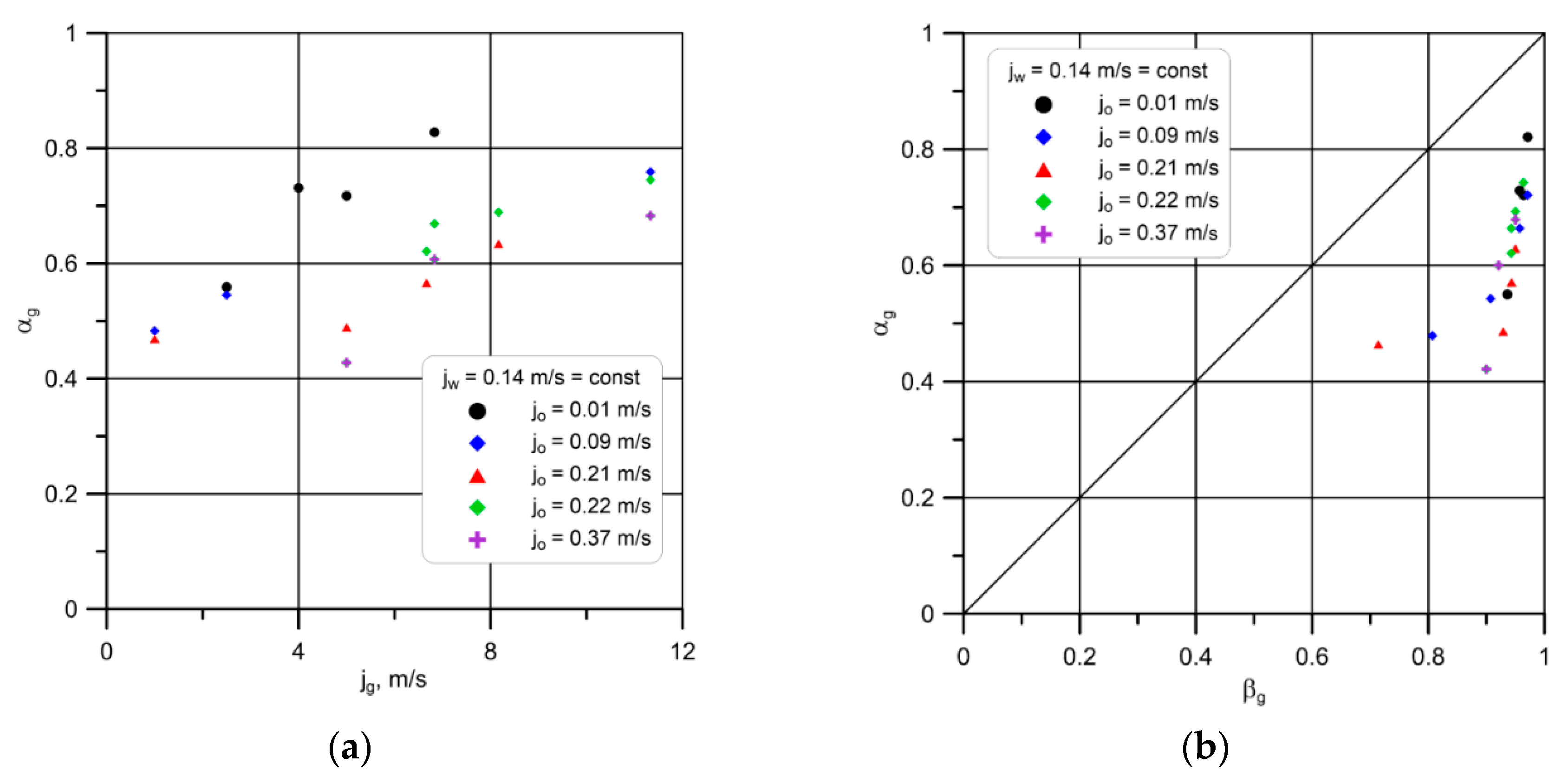
3.2. Void and Volume Fraction

In the case of the co-current flow of three non-mixing components such as air, oil and water, the flow rates of all these components have a mutual effect on the value of the actual void fraction of the phases, α_i. The values of the phase void fraction are affected by the values of the superficial velocities of all phases, j_i, in the flow, the physicochemical properties of individual components of the mixture and their mutual relations, as well as the type of liquid phase (oil, water) forming the dominant phase in the multiphase flow.

Based on the results of experimental research on the hydrodynamics of multiphase air–water–oil annular flow, an analysis of the influence of selected flow parameters on the value of the volume ratio of individual phases was performed. Due to the occurrence of many variables in this type of flow, and for the purpose of the graphical presentation of results, the superficial velocity of one of the components of the mixture was assumed to be a constant parameter characterizing the three-phase mixture, whereas the remaining superficial velocity values were considered to be variable. Due to the wide range of variations in flow parameters adopted in the study, only selected examples of the variations occurring in this type of flow are illustrated. Figure 4, Figure 5 and Figure 6 contain graphs providing examples of relations between the superficial flow velocities of individual components of the three-phase mixture and the values of the phase void fraction, as well as between the values of the actual void fraction of a particular component of the mixture, α_i, and the value of its void fraction at the inlet β_i.

The analysis of experimental data demonstrates that irrespective of the liquid phase that is dominant in the flow (water or oil), the void fraction of gas α_g increases with the increase in the superficial gas velocity, with a note that this value decreases for the case when the superficial velocity of any of the liquids increases (Figure 4). The study also found that the values of the air void fraction α_g are smaller than the corresponding values of the inlet void fraction β_g resulting from the relations representing the flow rates fed into the measuring channel. These differences are greater for the case of the oil-dominated flow. For the cases of volume ratios of oil, α_o, (Figure 5) and water, α_w, (Figure 6), it was found that these values increase along with greater superficial oil and water velocities, respectively, following the increases in the superficial gas phase velocity contributing to the decrease in the volume flow rates of each of the liquid phases. The analysis of the variations in α_o and α_w demonstrates that they assume a range of values that is greater than the one resulting from the volume feed rates given at the inlet to the channel (β_o, β_w), which indicates that each of these phases is accumulated in the channel, respectively. The reason for this accumulation is associated with the deceleration of the liquid phase resulting from its contact with the channel wall, with a greater effect of liquid holdup taking place during the flow with the dominant oil phase, and along with the increase in the oil viscosity.

When we take into account the entire range of the experimental data, we can state that in each case the values of the void and volume ratios of the individual phases of the three-phase flows are significantly affected by the superficial velocities of individual components; however, due to the interfacial slip occurring in the flow and the phase inversion phenomenon, the influence of these parameters on the values of the volume ratios of individual components does not offer completely unambiguous conclusions.

On the basis of the data recorded from the experiments concerned with the actual void and volume fractions of three-phase air–water–oil flow, an analysis was carried out to verify the performance of the selected calculation methods. Due to the fact that the literature to this date does not provide insights into the downward three-phase flow in the vertical channel, an attempt was made to adapt selected methods for calculating the phase volume ratios in the gas–liquid two-phase flow to determine this amount in the gas–liquid three-phase flow. The most frequently cited calculation methods in the literature were selected for assessment, whose high accuracy in calculating the value of gas volume share in gas–liquid two-phase flows has been confirmed for a large experimental database. In this respect, a variety of methods were identified by application of computational models, including the methods devised by Stomma [34], Chisholm [35], Armand [36], Zivi [37], Zhao et al. [38] and Harrison et al. [39], which were derived on the basis of the Lockhart–Martinelli parameter as well as its derivative, as well as the methods by Zuber-Findlay [40], Hughmark [41], GE RAMP [42] and Bonnecaze et al. [43], based on drift-flux.

For the purpose of determining the values of the void and volume fraction of the particular phases in the downward three-phase flow, another two methods were applied (Lahey [44], Pendyk [45] and Witczak et al. [46]), which are normally feasible for three-phase flows through horizontal pipes, as well as the Nowak method [24,25], which was developed specifically for three-phase flows through vertical pipes, and whose detailed reports can be found in the work reported by Pietrzak et al. [26]. The detailed description of relations applied to compute the void and volume fraction are summarized in

Table 6. Equations applied for the calculation of the void fraction in downward three-phase gas–liquid–liquid flow (vertical pipes).

Author	Equation
Methods for Gas–liquid Two-Phase Flow
$j_l=j_o+j_w$; $j_{3P}=j_g+j_o+j_w$; ${\beta }_g=\frac{j_g}{j_g+j_{l,}}$; $x=\frac{{\rho }_g{j}_g}{{\rho }_g{j}_g+{\rho }_l{j}_l}$
Stomma [34], (1979)	${\alpha }_g=1-\frac{{\beta }_g^2-x^2}{2\left[ln\left(\frac{1-x}{1-{\beta }_g}\right)-\left({\beta }_g-x\right)\right]}$
Chisholm [35], (1967)	${\alpha }_g=\frac{1}{1+S\frac{1-x}{x}\frac{{\rho }_g}{{\rho }_l}}$, $S={\left[x\frac{{\rho }_l}{{\rho }_g}+\left(1-x\right)\right]}^{0.5}$
Armand [36], (1946)	${\alpha }_g=1-\frac{4+\frac{8}{7}m}{5+m\left(\frac{{\beta }_g}{1-{\beta }_g}+\frac{8}{7}\right)}$ $m=4{Re}_l^{1/8}{\left(\frac{{\rho }_g}{{\rho }_l}\right)}^{0.5}\left[0.69+\left(1-{\beta }_g\right)\left(4+21.9\sqrt{F{r}_l}\right)\right]$ ${Re}_l=\frac{j_{l}d{\rho }_l}{{\eta }_l}$; $F{r}_l=\frac{j_l^2}{gd}$
Zivi [37], (1964)	${\alpha }_g=\frac{1}{1+\left(\frac{1-x}{x}\right){\left(\frac{{\rho }_g}{{\rho }_l}\right)}^{0.67}}$
Zhao et al. [38], (2001)	${\alpha }_g=\frac{1}{1+{\alpha }_g^{-0.125}{\left[\left(\frac{1-x}{x}\right)\left(\frac{{\rho }_g}{{\rho }_l}\right)\left(\frac{{\eta }_l}{{\eta }_g}\right)\right]}^{0.875}}$
Harrison et al. [39], (1975)	${\alpha }_g=\frac{1}{1+{\left(\frac{1-x}{x}\right)}^{0.8}{\left(\frac{{\rho }_g}{{\rho }_l}\right)}^{0.515}}$
Zuber-Findlay [40], (1965)	$\frac{j_g}{{\alpha }_g}=1.2j_{3P}+j_{g-3P}$; $j_{g-3P}=1.53{\left(\frac{g{\sigma }_l\left({\rho }_l-{\rho }_g\right)}{{\rho }_l^2}\right)}^{0.25}$
Hughmark [41], (1965)	${\alpha }_g=\frac{j_g}{1.2j_{3P}}$
GE RAMP [42], (1977)	$R_g=\frac{j_{g,0}}{C_g\left(j_g+j_l\right)+j_{g-3P}}$ $C_g=1.13$ for ${\alpha }_{g,exp}\le 0.65$ or $C_g=1+0.13\frac{1-{\alpha }_{g,exp}}{1-0.65}$ for ${\alpha }_{g,exp}>0.65$ $j_{g-3P}=2.9{\left(\frac{g{\sigma }_l\left({\rho }_l-{\rho }_g\right)}{{\rho }_l^2}\right)}^{0.25}$ for ${\alpha }_{g,exp}\le 0.65$ $j_{g-3P}=2.9{\left(\frac{g{\sigma }_l\left({\rho }_l-{\rho }_g\right)}{{\rho }_l^2}\right)}^{0.25}\left(\frac{1-{\alpha }_{g,exp}}{1-0.65}\right)$ for ${\alpha }_{g,exp}>0.65$
Bonnecaze et al. [43], (1971)	${\alpha }_g=\frac{j_g}{\left[1.2j_{3P}+0.35\sqrt{gd}\left(1-\frac{{\rho }_g}{{\rho }_l}\right)\right]}$
Methods for Gas–Liquid–Liquid Three-Phase Flow
Lahey [44], (1992)	${\alpha }_g=\frac{j_g}{1.164j_{3P}+0.457}$; ${\alpha }_w=\frac{j_w\left(1-{\alpha }_g\right)}{1.034j_w+0.0104}$; ${\alpha }_o=1-\left({\alpha }_g+{\alpha }_w\right)$.
Pendyk [45], (2002)	${\alpha }_g=\frac{{\beta }_g^{0.37}}{1+{(\frac{1}{{\beta }_g}-1)}^{0.5}}{\left(\frac{1-{\beta }_w}{1+{\beta }_o}\right)}^{0.43}$; ${\alpha }_w={\left({\beta }_w^{*}\right)}^{0.8}\left(1-{\alpha }_g\right)$; ${\alpha }_o=1-\left({\alpha }_g+{\alpha }_w\right)$.
Nowak [24], (2007)	${\alpha }_g=\frac{j_g}{\left[1+0.481{(1-{\beta }_g)}^{0.172}\right]j_{3P}+j_{g-3P}}$$j_{g-3P}=1.41{\left(\frac{g{\sigma }_w\left({\rho }_w-{\rho }_g\right)}{{\rho }_w^2}\right)}^{0.25}{(1-{\beta }_g^{*})}^3$ for ${\beta }_o^{*}<{\beta }_{o,cr}^{*}$ $j_{g-3P}=1.41{\left(\frac{g{\sigma }_o\left({\rho }_o-{\rho }_g\right)}{{\rho }_o^2}\right)}^{0.25}{(1-{\beta }_g^{*})}^3$ for ${\beta }_o^{*}\ge {\beta }_{o,cr}^{*}$ ${\alpha }_w=\frac{j_w\left(1-{\alpha }_g\right)}{\left[1+0.175{\left(1-{\beta }_w^{*}\right)}^{0.151}\right]j_l-j_{w-l}}$; ${\alpha }_o=1-{\alpha }_g-{\alpha }_w$ $j_{w-l}=1.41{\left(\frac{g\left({\sigma }_w-{\sigma }_o\right)\left({\rho }_w-{\rho }_o\right)}{{\rho }_w^2}\right)}^{0.25}{\left(1-{\beta }_w^{*}\right)}^3$; ${\epsilon }_{o,cr}^{*}=\frac{{\epsilon }_{o,inw}^{*}}{1+8.2 \times {10}^{-4}R{e}_g^{0.472}}$

.

In order to determine the applicability of the selected methods (developed for two-phase gas–liquid flow) for the calculation of the gas void fraction in the three-phase gas–liquid–liquid flow, this flow was considered as a pseudo-two-phase gas–liquid mixture flow. In this flow, the liquid components of the mixture, water and oil, were considered to play the role of a liquid phase with equivalent properties. In this case, the properties of the liquid mixture were calculated by taking into account the volume fraction of oil and water in the two-phase liquid mixture in accordance with the following relation:

$${\rho }_l={\beta }_o^{*}{\rho }_o+{\beta }_w^{*}{\rho }_w, {\eta }_l={\beta }_o^{*}{\eta }_o+{\beta }_w^{*}{\eta }_w, {\sigma }_l={\beta }_o^{*}{\sigma }_o+{\beta }_w^{*}{\sigma }_w,$$

(6)

The accuracy of the calculation methods was assessed by comparing the measured values of gas void fraction derived as a result of the experiments with the values calculated in accordance with the methods described in Table 6. This comparison involved the determination of the mean values of MRE (mean relative error) and MAE (mean absolute error) representing the relative error, and the determination of the percentage ratio of the number of experimental points included in the specified range of MRE values. These values were calculated according to the following relations:

$$MRE=\frac{1}{N}{\displaystyle \sum _{k=1}^N\frac{{\alpha }_{i,cal}-{\alpha }_{i,exp}}{{\alpha }_{i,exp}}}100\%$$

(7)

$$MAE=\frac{1}{N}{\displaystyle \sum _{k=1}^N\left|\frac{{\alpha }_{i,cal}-{\alpha }_{i,exp}}{{\alpha }_{i,exp}}\right|}100\%$$

(8)

The results of the statistical analysis of the data are presented in

Table 7. Results of statistical analysis of methods applied to the calculation of α_g.

No	Author	Value of Statistical Quantities, %
		MRE	MAE	Percent Ratio of Points for MAE <30%
Methods for two-phase gas–liquid flow
1.	Stomma [34]	21.91	23.26	74.6
2.	Chisholm [35]	14.58	16.73	82.2
3.	Armand [36]	3.12	11.99	87.7
4.	Zivi [37]	−12.95	21.80	71.0
5.	Zhao et al. [38]	10.59	17.74	82.3
6.	Harrison et al. [39]	−17.46	21.18	69.9
7.	Zuber-Findlay [40]	4.89	14.60	86.7
8.	Hughmark [41]	11.26	16.99	82.9
9.	GE RAMP [42]	10.53	15.59	87.2
10.	Bonnecaze et al. [43]	7.94	15.42	86.8
Methods for three-phase gas–liquid–liquid flow
11.	Lahey [44]	4.53	13.54	88.0
12.	Pendyk [45]	9.61	14.80	86.9
13.	Nowak [24]	4.32	12.96	90.0

.

On the basis of the statistical assessment, we can see that the best compliance of the calculations was obtained for the methods proposed by Armand [36], Zuber-Findlay [40], GERAMP [42] and Bonnecaze et al. [43], for which more than 85% of the points were in the range of ±30% of the mean relative error (MRE). Good results were obtained by comparing the values of the measured void and volume fraction with the calculations according to the method of Chisholm [35], Hughmark [41] and Zhao et al. [38], for which this value is over 82%. On the other hand, the methods of Harrison et al. [39] and Chisholm [35] were much less accurate in calculations for which only 69.9–74.5% of the points were within the range of ±30% of the mean relative error, MRE.

Considerable levels of accuracy in calculating α_g values are provided by the methods developed by Lahey [44] and Pendyk [45] for the gas–liquid–liquid three-phase flow in horizontal channels, and by the Nowak method [24], which is valid for upward three-phase flow through a vertical channel. The results of statistical calculations for these methods are presented in Figure 7, Figure 8 and Figure 9.

On the basis of the curves presented in Figure 7, Figure 8 and Figure 9, we can conclude that each of these methods provides a more than 85% ratio of points within 30% of the value of the mean relative error in relation to calculating the value of the gas void fraction, α_g. Unfortunately, all of the investigated models are characterized by a low accuracy in calculating the value of volume fractions of water, α_w, and oil, α_o. This is probably due to the fact that for the case of three-phase downflow, there is a different distribution of oil and water in the liquid film from the one in the flow in horizontal pipes, and in the upflow of the three-phase mixture through vertical pipes.

When we consider the complexity of the phenomena occurring during the co-current downward three-phase air–water–oil flow through vertical pipes, a decision was made to adopt the calculation method for calculating the gas void fraction, which generated the highest accuracy of calculations of this quantity, and at the same time provided good results for high oil viscosities.

Taking into account the complexity of the phenomena accompanying the co-current downward air–water–oil three-phase flow in the vertical pipes, a new method for calculating the volume fraction of gas, water and oil was developed. The method gives the highest accuracy in the void fraction calculations. The drift-flux model was adopted as the basis for the development of a new method for calculating the gas volume fraction in air–water–oil three-phase flow, which enables the specificity of a multiphase flow with high viscosity oil to be taken into account.

The high accuracy of the calculation methods based on the drift-flux model was also confirmed by other authors, such as Czernek et al. [47,48], that have investigated the gas–liquid downward flow in vertical pipes for different oils with viscosities in the range of 90–3500 mPas.

The gas void fraction, α_g, according to the new developed method, should be calculated as:

$${\alpha }_g=\frac{j_g}{1.65{(1-{\beta }_g)}^{0.075}{j}_{3P}+j_{g-3P}}$$

(9)

where

$$j_{g-3P}=1.41{\left(\frac{g{\sigma }_l\left({\rho }_l-{\rho }_g\right)}{{\rho }_l^2}\right)}^{0.25}{(1-{\beta }_g)}^3$$

(10)

The liquid phase properties were assumed to be equivalent to the properties of liquid, where the real volume fractions of water and oil are taken into account:

$${\rho }_l={\alpha }_o^{*}{\rho }_o+{\alpha }_w^{*}{\rho }_w; {\sigma }_l={\alpha }_o^{*}{\sigma }_o+{\alpha }_w^{*}{\sigma }_w$$

(11)

In turn, the volume fraction of water (as the liquid with the lower viscosity) is proposed to be derived from the following relation:

$${\alpha }_w=\left(1-{\alpha }_o^{*}\right)\left(1-{\alpha }_g\right)$$

(12)

whereas the value for oil, as the compliment to one, is taken as the total of the volume fraction of the phases in the three-phase flow:

$${\alpha }_o=1-\left({\alpha }_g+{\alpha }_w\right)$$

(13)

In the conditions of the decay of the gas phase flow, i.e., for α_g = 0, Equations (12) and (13) play the role of the method applicable for calculating the actual values of the water and oil void fraction for liquid–liquid two-phase flow:

$${\alpha }_w^{*}=1-{\alpha }_o^{*}$$

(14)

where

$${\alpha }_o^{*}=\frac{1}{1+1.109F{r}_o^{0.25}F{r}_w^{0.17}\frac{1-{\beta }_o^{*}}{{\beta }_o^{*}}}$$

(15)

$$F{r}_o=\frac{j_o^2}{gd} ; F{r}_w=\frac{j_w^2}{gd}$$

(16)

The values of the Froud number in Equation (15) changed in the range of Fr_o = (5 × 10⁻⁵–1.178) and Fr_w = (0.0021–17.87), and were a measure of the interfacial slip in the oil–water liquid film.

The comparison of the measured values of the volume and void fraction of air, water and oil, along with the values corresponding to them derived on the basis of the proposed method, are presented in Figure 10 and Figure 11.

From the distribution of points on the graph (Figure 10a), we can see that almost 92% of the measuring points are within the limit of the mean relative error, MRE = ±30%, regardless of the type and physical properties of the oil analyzed in the experiment.

On the other hand, the graph presented in Figure 10b, which contains a comparison of the measured and calculated values of the volume ratios of water, demonstrates that approximately 66% of the measuring points are within the limit of the mean relative error, MRE = ±30%. In this case, the highest percentage of this value was obtained compared to the previously investigated calculation methods.

On the other hand, on the basis of the distribution of points in Figure 10c, presenting the comparison of the measured and calculated values of the oil volume ratios in this case, the results with regard to more than 53% of the measurement points contained in the range of the mean relative error MRE = ±30% were obtained. It was also noticed that a better accuracy of calculations was obtained for higher values of the oil volume fraction. This corresponded to the region of dominance of the oil phase in the flow.

On the basis of the comparison of the accuracy of the calculations of the void fraction of the specific phases in a three-phase mixture, presented in Figure 11, it can be concluded that the newly developed method for the calculation of the void fraction for particular phases in a co-current downward three-phase gas–liquid–liquid flow provides a very high accuracy of calculations, regardless of the dominant liquid phase in the flow.

4. Conclusions

The present studies are concerned with the identification of multiphase flow patterns and the determination of the void fraction of individual phases. The experimental results constitute a complement to and an extension of the current state of knowledge in relation to the hydrodynamics of three-phase gas–liquid–liquid downward annular flow, especially with liquids with high viscosity.

During the tests, seven three-phase flow patterns were identified: drops of dispersed oil in water (A-DrDO/W), dispersed oil foam in water (A-FDO/W), and water dispersed in oil (A-DO/W), drops of water in oil (A-DrDW/O), intermittent water dispersed in oil (A-IDW/O) and water dispersed in oil (A-DW/O), as well as emulsified flow A-(O + W). The patterns characterized in the work were used to develop a new flow regime map. A new flow regime map is a useful tool for getting an overview of which types of flow patterns can be expected for a particular set of flow parameters, taking into account the dominance of the water or oil phase in the flow. This map takes into account both the areas of occurrence of the two-phase liquid–liquid and three-phase gas–liquid–liquid flow patterns. The map for the oil–water–air three-phase flow is valid for the following conditions: j_3P = 0.35–53.4 m/s and β_o * = 0.48–94%. In the case of a downward annular oil–water two-phase flow, this map is valid for j_l = 0.052–2.14 m/s and β_o * = 0.48–94%.

The new flow map, and relations pertaining to the calculation of the void fraction of phases presented in the work, form the first study in the literature concerned with the description of the conditions of the downward air–water–oil three-phase flow through vertical pipes where such high viscosity oils were used.

The results of the research and analysis presented in the paper can be applied to complement experimental works performed further in this area, as well as in engineering calculations.

References

1. Cyklis, P. Industrial scale engineering estimation of the heat transfer in falling film juice evaporators. Appl. Therm. Eng. 2017. [Google Scholar] [CrossRef]
2. Czernek, K.; Płaczek, M. Hydrodynamics of two-phase flow in tubular reactor. Czas. Tech. 2017, 8, 101–114. [Google Scholar] [CrossRef]
3. Nagavarapu, A.K.; Garimella, S. Experimentally validated models for falling-film absorption around microchannel tube banks: Heat and mass transfer. Int. J. Heat Mass Transf. 2019. [Google Scholar] [CrossRef]
4. Witczak, S.; Troniewski, L.; Filipczak, G. Influence of oil concentration on heat transfer conditions during pool boiling of water-oil mixtures. Chem. Process. Eng. Inz. Chem. Proces. 2008, 29, 859–867. [Google Scholar]
5. Czernek, K.; Witczak, S. Non-invasive evaluation of wavy liquid film. Chem. Process. Eng. Inz. Chem. Proces. 2013, 34. [Google Scholar] [CrossRef] [Green Version]
6. Dong, C.; Hibiki, T. Correlation of heat transfer coefficient for two-component two-phase slug flow in a vertical pipe. Int. J. Multiph. Flow 2018, 108. [Google Scholar] [CrossRef]
7. Hamidi, M.J.; Karimi, H.; Boostani, M. Flow patterns and heat transfer of oil-water two-phase upward flow in vertical pipe. Int. J. Therm. Sci. 2018, 127, 173–180. [Google Scholar] [CrossRef]
8. Guichet, V.; Jouhara, H. Condensation, evaporation and boiling of falling films in wickless heat pipes (two-phase closed thermosyphons): A critical review of correlations. Int. J. Thermofluids 2020, 1–2, 100001. [Google Scholar] [CrossRef]
9. Sobolewski, M.; Fuchs, L. Consistency issues of Lagrangian particle tracking applied to a spray jet in crossflow. Int. J. Multiph. Flow 2007, 33, 394–410. [Google Scholar] [CrossRef] [Green Version]
10. Edwards, L.; Jebourdsingh, D.; Dhanpat, D.; Chakrabarti, D.P. Hydrodynamics of air and oil–water dispersion/emulsion in horizontal pipe flow with low oil percentage at low fluid velocity. Cogent Eng. 2018, 5, 1494494. [Google Scholar] [CrossRef]
11. Edwards, L.; Darryan, D.; Chakrabarti, D.P. Hydrodynamics of three phase flow in upstream pipes. Cogent Eng. 2018, 5, 1433983. [Google Scholar] [CrossRef]
12. Edwards, L.; Keeran, W.; Chakrabarti, D.P. Phase inversion in liquid phase for air-liquid horizontal flow. Cogent Eng. 2020, 7, 1782622. [Google Scholar] [CrossRef]
13. Poettmann, F.H.; Carpenter, P.G. The Multiphase Flow of Gas, Oil, and Water Through Vertical Flow Strings with Application to the Design of Gas-lift Installations. In Proceedings of the Drilling and Production Practice, New York, NY, USA, 1 January 1952; American Petroleum Institute: Washington, DC, USA, 1952. [Google Scholar]
14. Tek, M.R. Multiphase Flow of Water, Oil and Natural Gas Through Vertical Flow Strings. J. Pet. Technol. 1961. [Google Scholar] [CrossRef]
15. Foreman, F.J.; Woods, P.H. Void fraction calculations for three phase flow in a vertical pipe. Proj. Rep. Course 1975, 2. [Google Scholar]
16. Shean, A.R. Pressure drop and phase fraction in oil-water-air vertical pipe flow. Mech. Eng. 1976. Available online: https://dspace.mit.edu/handle/1721.1/30976 (accessed on 14 August 2020).
17. Pleshko, A.; Sharma, M.P. An experimental study of vertical three-phase (oil-water-air) upward flows. Winter Annu. Meet. ASME Dallas 1990, 97–108. [Google Scholar]
18. Woods, G.S.; Speddeng, P.L.; Watterson, J.K.; Raghunathan, R.S. Three-phase oil/water/air vertical flow. Chem. Eng. Res. Des. 1998. [Google Scholar] [CrossRef]
19. Spedding, P.L.; Woods, G.S.; Raghunathan, R.S.; Watterson, J.K. Flow pattern, holdup and pressure drop in vertical and near vertical two- and three-phase upflow. Chem. Eng. Res. Des. 2000. [Google Scholar] [CrossRef]
20. Oddie, G.; Shi, H.; Durlofsky, L.J.; Aziz, K.; Pfeffer, B.; Holmes, J.A. Experimental study of two and three phase flows in large diameter inclined pipes. Int. J. Multiph. Flow 2003. [Google Scholar] [CrossRef]
21. Shi, H.; Holmes, J.A.; Diaz, L.R.; Durlofsky, L.J.; Aziz, K. Drift-flux parameters for three-phase steady-state flow in wellbores. SPE J. 2005, 10, 130–137. [Google Scholar] [CrossRef]
22. Descamps, M.; Oliemans, R.V.A.; Ooms, G.; Mudde, R.F.; Kusters, R. Influence of gas injection on phase inversion in an oil-water flow through a vertical tube. Int. J. Multiph. Flow 2006. [Google Scholar] [CrossRef]
23. Descamps, M.N.; Oliemans, R.V.A.; Ooms, G.; Mudde, R.F. Experimental investigation of three-phase flow in a vertical pipe: Local characteristics of the gas phase for gas-lift conditions. Int. J. Multiph. Flow 2007. [Google Scholar] [CrossRef]
24. Nowak, M. Void Fractions and Three-Phase Pressure Drop in Vertical Pipe. Ph.D. Thesis, Opole University of Technology, Opole, Poland, 2007. (In Polish). [Google Scholar]
25. Nowak, M.; Troniewski, L.; Witczak, S. Prediction of void fraction in three-phase air–water–oil upflow. In Proceedings of the 5th International Conference on Transport Phenomena in Multiphase Systems, HEAT 2008, Bialystok, Poland, 30 June–3 July 2008; Bialystok Technical University: Bialystok, Poland, 2008; Volume 1, pp. 349–356. [Google Scholar]
26. Pietrzak, M.; Płaczek, M.; Witczak, S. Upward flow of air–oil–water mixture in vertical pipe. Exp. Therm. Fluid Sci. 2017. [Google Scholar] [CrossRef]
27. Colmanetti, A.R.A.; de Castro, M.S.; Barbosa, M.C.; Rodriguez, O.M.H. Phase inversion phenomena in vertical three-phase flow: Experimental study on the influence of fluids viscosity, duct geometry and gas flow rate. Chem. Eng. Sci. 2018. [Google Scholar] [CrossRef]
28. Wang, S.; Zhang, H.; Sarica, C.; Pereyra, E.J. Experimental Study of High-Viscosity Oil/Water/Gas Three-Phase Flow in Horizontal and Upward Vertical Pipes. SPE Prod. Oper. 2013, 28, 306–316. [Google Scholar] [CrossRef]
29. Bannwart, A.C.; Rodriguez, O.M.H.; Trevisan, F.E.; Vieira, F.F.; de Carvalho, C.H.M. Experimental investigation on liquid–liquid-gas flow: Flow patterns and pressure-gradient. J. Pet. Sci. Eng. 2009. [Google Scholar] [CrossRef]
30. Huang, S.; Zhang, B.; Lu, J.; Wang, D. Study on flow pattern maps in hilly-terrain air–water–oil three-phase flows. Exp. Therm. Fluid Sci. 2013. [Google Scholar] [CrossRef]
31. Hanafizadeh, P.; Shahani, A.; Ghanavati, A.; Akhavan-Behabadi, M.A. Experimental investigation of air-water-oil three-phase flow patterns in inclined pipes. Exp. Therm. Fluid Sci. 2017. [Google Scholar] [CrossRef] [Green Version]
32. Brandt, A. The Annular Flow of Multiphase Mixture in Pipes of Film-Type Evaporators. Ph.D. Thesis, Opole University of Technology, Opole, Poland, 2015. (In Polish). [Google Scholar]
33. Goshika, B.K.; Majumder, S.K. Entrainment and holdup of gas–liquid–liquid dispersion in a downflow gas–liquid–liquid contactor. Chem. Eng. Process. Process. Intensif. 2018. [Google Scholar] [CrossRef]
34. Stomma, Z. Two-Phase Flows-Void Fraction Values Determination; No. INR--1818/9/R; Institute of Nuclear Research: Kyiv, Ukraine, 1979; Volume 12. [Google Scholar]
35. Chisholm, D. A theoretical basis for the Lockhart-Martinelli correlation for two-phase flow. Int. J. Heat Mass Transf. 1967. [Google Scholar] [CrossRef]
36. Armand, A.A. Resistance to two-phase flow in horizontal tubes. Izv. Vsa. Tepl. Inst. 1946, 15, 16–23. [Google Scholar]
37. Zivi, S.M. Estimation of steady-state steam void-fraction by means of the principle of minimum entropy production. J. Heat Transf. 1964. [Google Scholar] [CrossRef]
38. Zhao, T.S.; Bi, Q.C. Co-current air-water two-phase flow patterns in vertical triangular microchannels. Int. J. Multiph. Flow 2001. [Google Scholar] [CrossRef]
39. Harrison, R.F. Methods for the Analysis of Geothermal Two-Phase Flow. Master’s Thesis, University of Auckland, Aucklan, New Zealand, 1975. [Google Scholar]
40. Zuber, N.; Findlay, J.A. Average volumetric concentration in two-phase flow systems. J. Heat Transf. 1965. [Google Scholar] [CrossRef]
41. Hughmark, G.A. Holdup and heat transfer in horizontal slug gas–liquid flow. Chem. Eng. Sci. 1965. [Google Scholar] [CrossRef]
42. Punches, W.C. MAYU04: A Method to Evaluate Transient Thermal Hydraulic Conditions in Rod Bundles; General Electric Co.: Schenectady, NY, USA, 1977. [Google Scholar]
43. Bonnecaze, R.H.; Erskine, W.; Greskovich, E.J. Holdup and pressure drop for two-phase slug flow in inclined pipelines. AIChE J. 1971. [Google Scholar] [CrossRef]
44. Lahey, R.T.; Açikgöz, M.; França, F. Global volumetric phase fractions in horizontal three-phase flows. AIChE J. 1992. [Google Scholar] [CrossRef]
45. Pendyk, B. Void Fraction of Gas–liquid–liquid Flow in Horizontal Pipes. Ph.D. Thesis, Opole University of Technology, Opole, Poland, 2002. (In Polish). [Google Scholar]
46. Witczak, S.; Pendyk, B. The method of the hold-up calculation during the three-phase flow. Chem. Process. Eng. Inz. Chem. Proces. 2004, 25, 75–86. [Google Scholar]
47. Czernek, K. Hydrodynamic Aspects of Thin-Film Apparatus Design for Very Viscous Liquids; Oficyna Wydawnicza Politechniki Opolskiej: Opole, Poland, 2013; ISBN 8364056158. [Google Scholar]
48. Czernek, K.; Okoń, P. Verification of methods for calculating the gas volume fraction in the vertical descending flow of two-phase gas–liquid mixtures. J. Mech. Energy Eng. 2018. [Google Scholar] [CrossRef] [Green Version]
Figure 1. Experimental setup (a), cross-section of the test channel (b); 1—oil tank, 2—gear pump, 3 and 4—transparent experimental section of channel applied for flow pattern observation and registration, 5—shut-off valves, 6—shut-off gear, 7—ball valve, 8—battery of oil rotameters, 9—battery of water rotameters, 10—non-transparent section of channel, 11—battery of air rotameters, 12—reducing valve, 13 and 20—separators, 14—measuring cylinder, 15—measuring probes, 16—measurement card, 17—computer applied for data registration, 18—oil tank, 19—hydrophor. Feeding systems: C—oil, B—water, A—air, K—chamber for multi-phase mixture generation.
Energies 14 00030 g001
Figure 2. Actual waveforms of voltage variations during liquid–liquid flow: (a) water-dominated flow O/W, (b) emulsified oil O + W, (c) oil-dominated flow W/O.
Energies 14 00030 g002
Figure 3. Gas–liquid–liquid three-phase flow map for annular falling flow. Map including data related to liquid–liquid two-phase flow, combined with (a) distribution of experimental points, (b) areas corresponding to the occurrence of specific flow patterns.
Energies 14 00030 g003
Figure 4. Gas void fraction αg (oil viscosity ηo = 0.3 Pas) in the function of (a) superficial gas velocity, jg, and (b) value of gas void fraction at the channel inlet, βg.
Energies 14 00030 g004
Figure 5. Example applied to illustrate the dependence of oil volume ratio, αo, for oil viscosity of ηo = 0.3 Pas on (a) the value of the superficial oil velocity, jo, and (b) the value of water volume fraction at the channel inlet, βo.
Energies 14 00030 g005
Figure 6. Example applied to illustrate the relation between water volume fraction, αw, for oil viscosity of ηo = 0.3 Pas on (a) the value of superficial water velocity, jw, and (b) the value of the water volume fraction at the channel inlet, βw.
Energies 14 00030 g006
Figure 7. Analysis of method applied for determining the void and volume fraction of phases for downward three-phase oil–water–air flow (a), and (b) values of experimental points located within the boundary of <30% of the MAE of experimental points, in accordance with the Lahey et al. method [44].
Energies 14 00030 g007
Figure 8. Statistical analysis of method applied for determining void and volume fraction of phases for downward three-phase oil–water–air flow (a), and (b) values of experimental points located within the range of <30% of the MAE of experimental points, in accordance with the Pendyk method [45].
Energies 14 00030 g008
Figure 9. Statistical analysis of method applied for determining void and volume fraction of phases for downward three-phase oil–water–air flow (a), and (b) values of experimental points located within the range of <30% of the MAE of experimental points, in accordance with the Nowak method [24].
Energies 14 00030 g009
Figure 10. Comparison of measured and calculated values of void fraction for (a) gas αg, (b) water αw, and (c) oil αo, according to the proposed method.
Energies 14 00030 g010aEnergies 14 00030 g010b
Figure 11. Statistical analysis of the method applied for determining the values of void fraction of phases for downward three-phase oil–water–air flow (a), and (b) values of experimental points in the boundary of < 30% of the MAE in accordance with the proposed method.
Energies 14 00030 g011