Probabilistic Forecasting of Wind Turbine Icing Related Production Losses Using Quantile Regression Forests

 , , , , and
Abstract
1. Introduction
2. Data
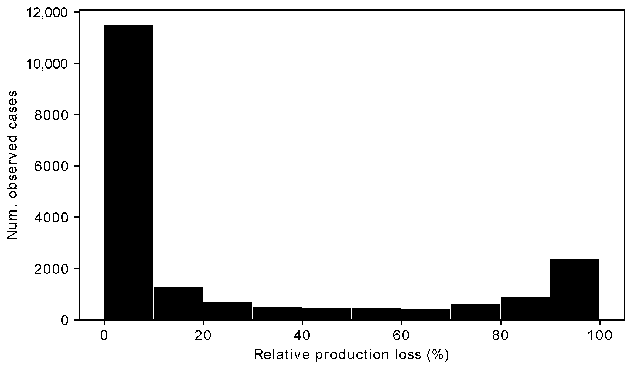
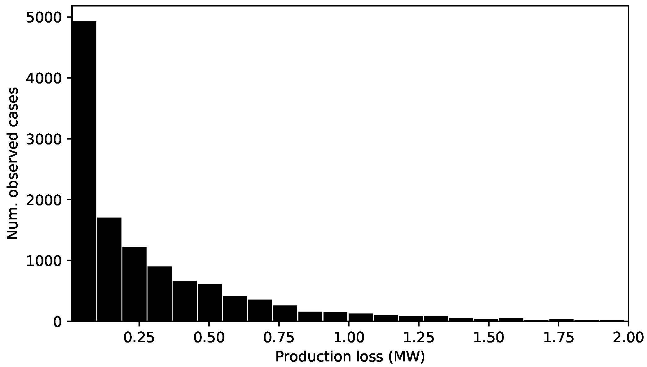
2.1. Observations
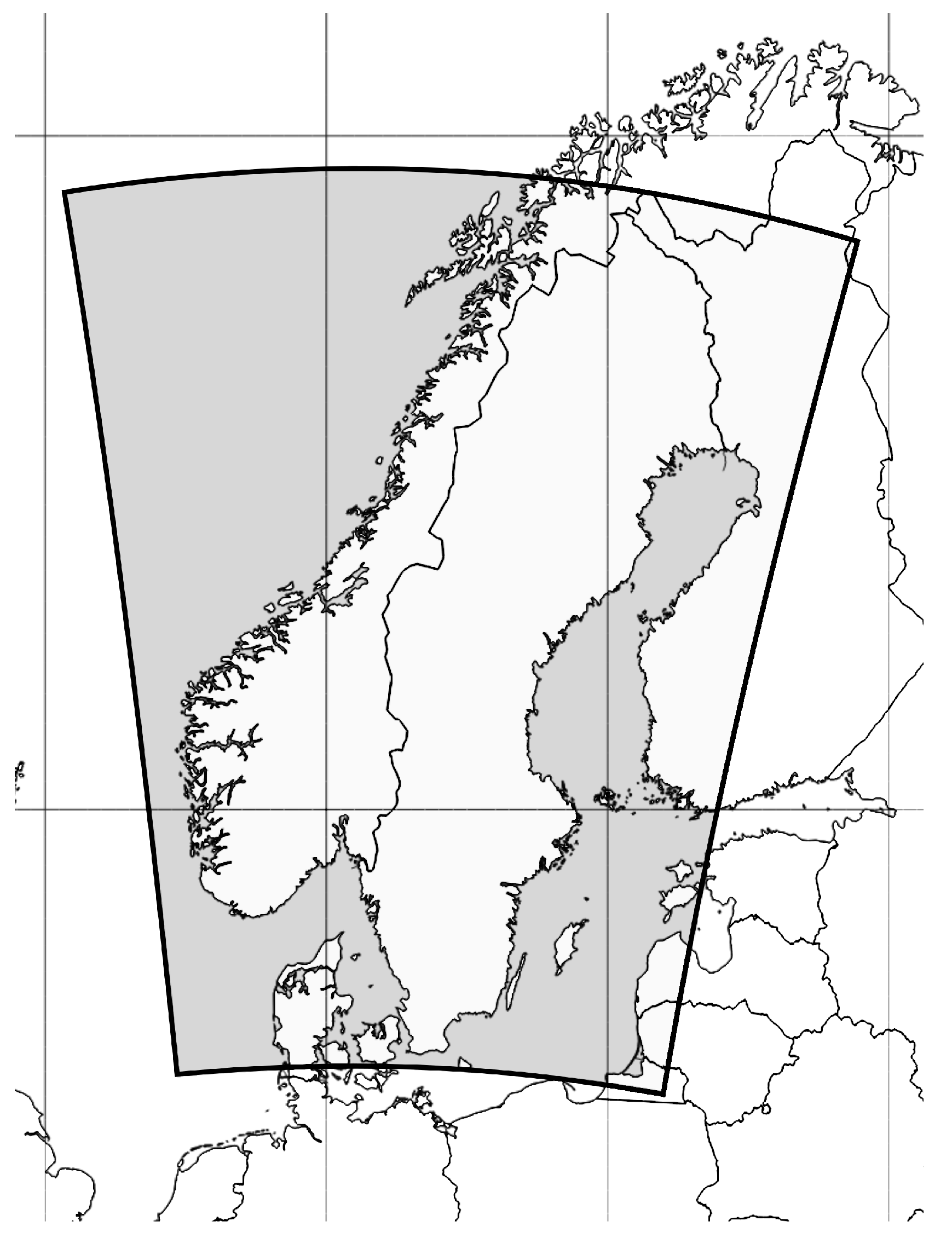
2.2. Numerical Weather Prediction Model
2.3. Icing Model
3. Method
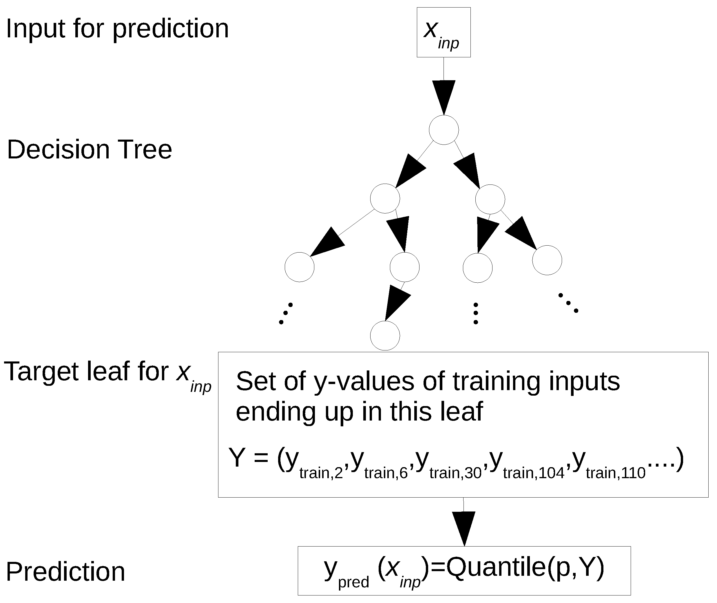
3.1. Machine Learning Method—Regression Forests
3.2. Training and Test Set Data
3.2.1. Training Features
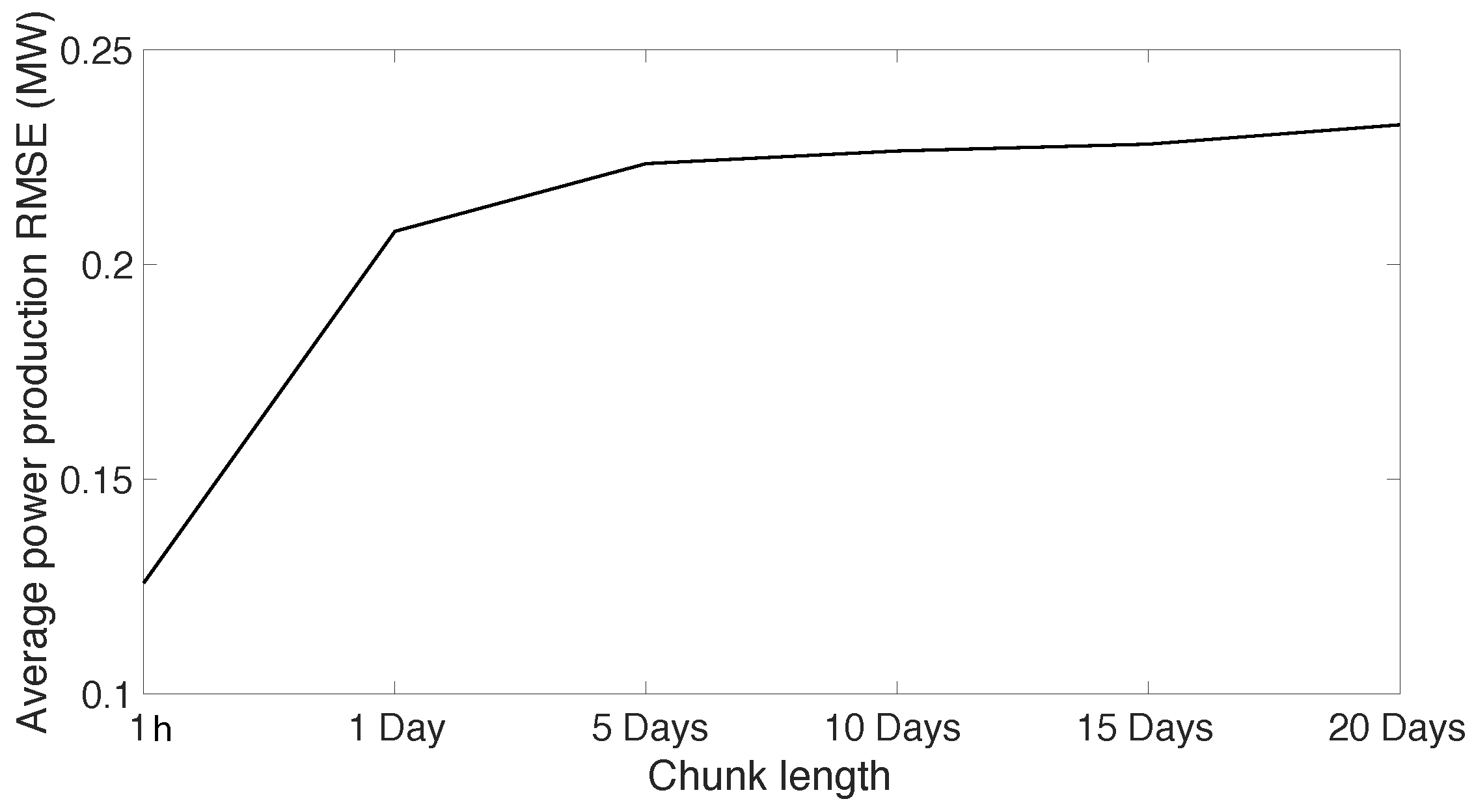
3.2.2. Splitting the Training and Test Data Using k-Fold cross Validation
3.2.3. Tuning of the Model
3.3. Reference Forecasts
4. Results
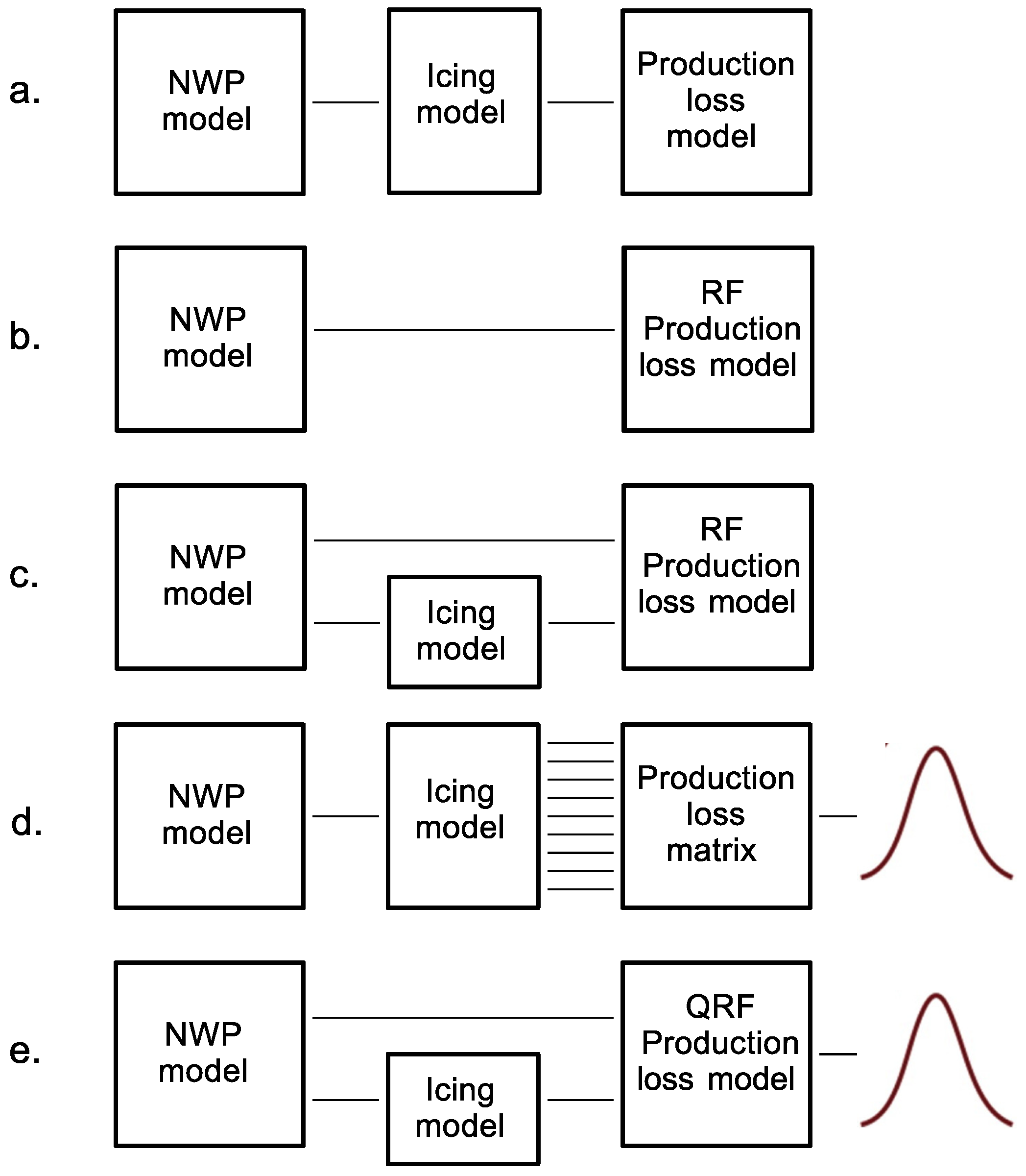
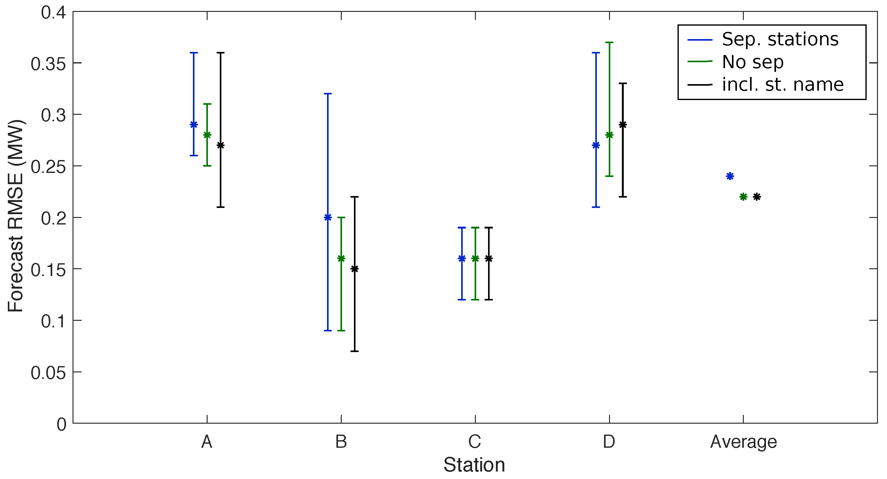
4.1. Adding the Icing Model to the Modelling Chain and Relative Importance of Input Parameters
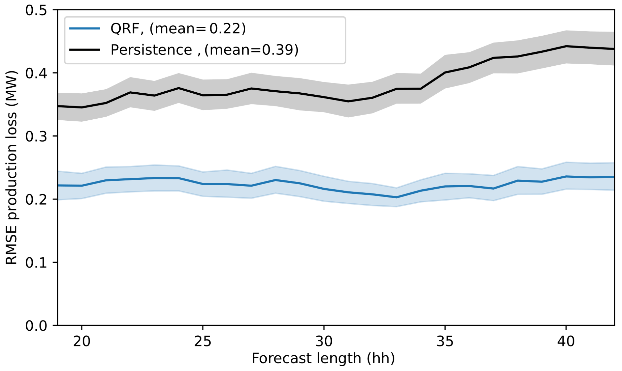
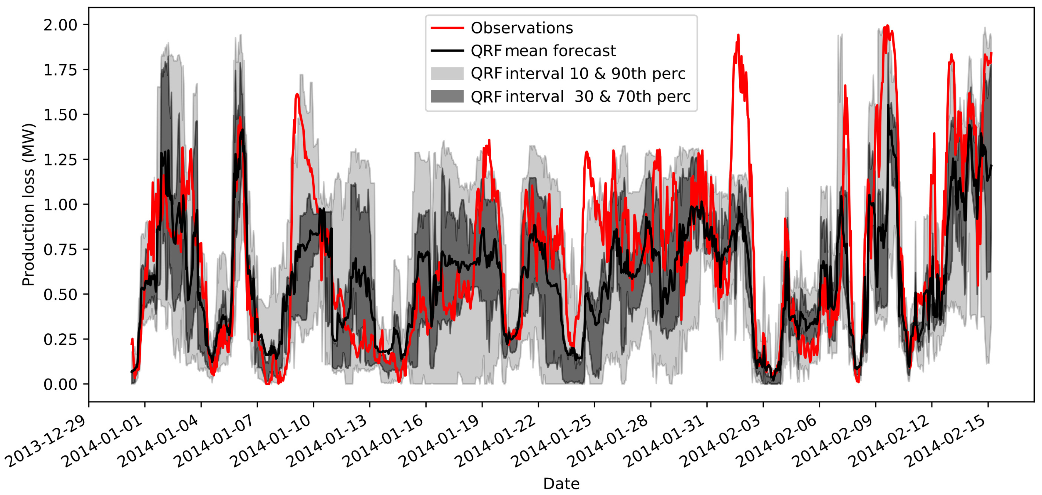
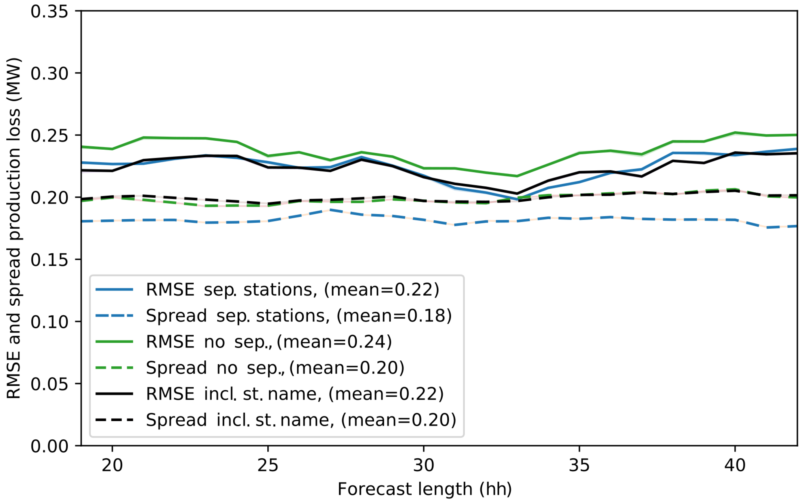
4.2. Deterministic Forecasts Skill
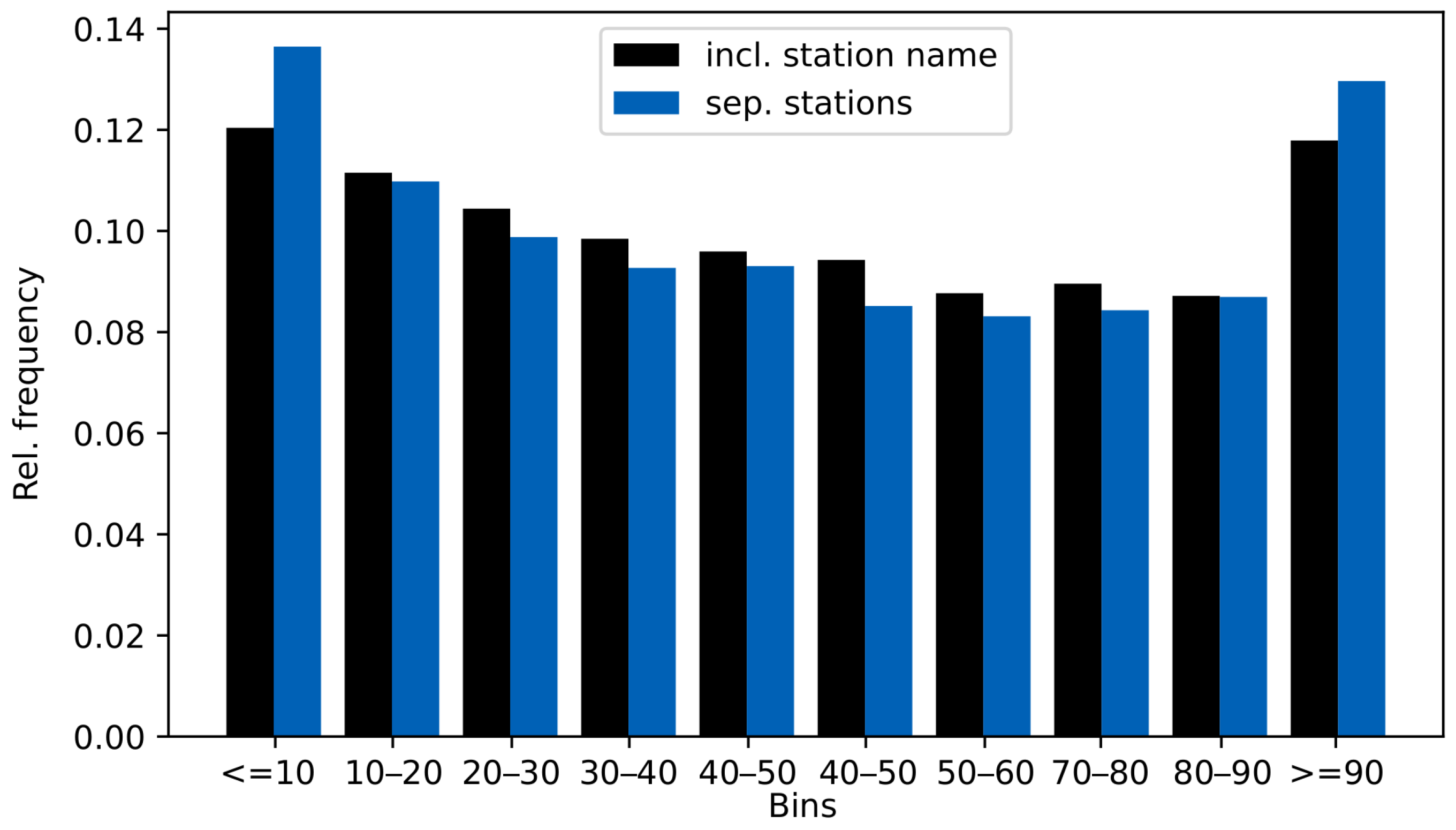
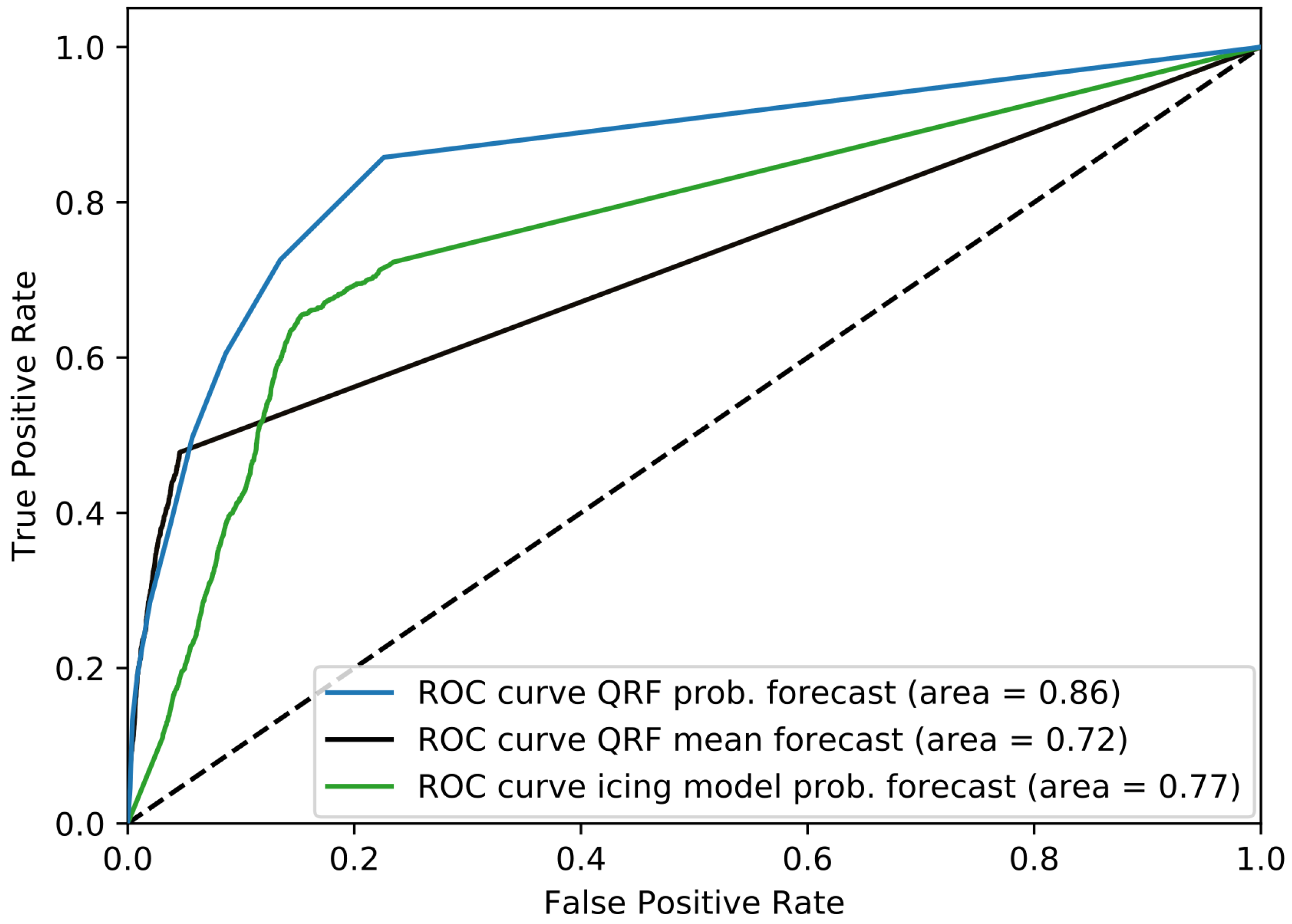
4.3. Probabilistic Forecast Skill
5. Discussion and Conclusions
Author Contributions
Funding
Institutional Review Board Statement
Informed Consent Statement
Data Availability Statement
Acknowledgments
Conflicts of Interest
Abbreviations
| MDPI | Multidisciplinary Digital Publishing Institute |
| DOAJ | Directory of open access journals |
| NWP | Numerical Weather Prediction |
| RF | Random Forest Regression |
| QRF | Quantile Regression Forest |
| probability density function | |
| RMSE | root mean square error |
| ROC | Receiver operating characteristics |
| MW | Megawatt |
References
- Lehtomaki, V. IEA Wind Task 19, “Emerging from the Cold”. 2016. Available online: https://www.windpowermonthly.com/article/1403504/emerging-cold (accessed on 10 February 2020).
- Kraj, A.G.; Bibeau, E.L. Phases of icing on wind turbine blades characterized by ice accumulation. Renew. Energy 2010, 35, 966–972. [Google Scholar] [CrossRef]
- Lehtomäki, V.; Krenn, A.; Ordaens, P.J.; Godreau, C.; Davis, N.; Khadiri-Yazami, Z.; Bredesen, R.E.; Ronsten, G.; Wickman, H.; Bourgeois, S.; et al. IEA Wind TCP Task 19, Available Technologies for Wind Energy in Cold Climates Report. Technical Report. 2018. Available online: https://community.ieawind.org/HigherLogic/System/DownloadDocumentFile.ashx?DocumentFileKey=6697b7bd-b175-12b0-ecbf-2558c35d309b&forceDialog=0 (accessed on 28 December 2020).
- Molinder, J.; Körnich, H.; Olsson, E.; Bergström, H.; Sjöblom, A. Probabilistic forecasting of wind power production losses in cold climates: A case study. Wind Energy Sci. 2018, 3, 667–690. [Google Scholar] [CrossRef]
- Davis, N.; Pinson, P.; Hahmann, A.N.; Clausen, N.E.; Žagar, M. Identifying and characterizing the impact of turbine icing on wind farm power generation. Wind Energy 2016, 16, 1503–1518. [Google Scholar] [CrossRef]
- Nygaard, B.E.K.; Àgústsson, H.; Somfalvi-Tóth, K. Modeling Wet Snow Accretion on Power Lines: Improvements to Previous Methods Using 50 Years of Observations. J. Appl. Meteorol. Climatol. 2013, 52, 2189–2203. [Google Scholar] [CrossRef]
- Makkonen, L. Models for the growth of rime, glaze icicles and wet snow on structures. Philos. Trans. R. Soc. Lond. 2000, 358, 2039–2913. [Google Scholar] [CrossRef]
- Molinder, J.; Körnich, H.; Olsson, E.; Hessling, J.P. The Use of Uncertainty Quantification for the Empirical Modeling of Wind Turbine Icing. J. Appl. Meteorol. Climatol. 2020, 58, 2019–2032. [Google Scholar] [CrossRef]
- Davis, N. Icing Impacts on Wind Energy Production. Ph.D. Thesis, DTU Wind Energy, Lyngby, Denmark, 2014. [Google Scholar]
- Thorsson, P.; Söderberg, S.; Bergström, H. Modelling atmospheric icing: A comparison between icing calculated with measured meteorological data and NWP data. Cold Reg. Sci. Technol. 2015, 119, 124–131. [Google Scholar] [CrossRef]
- Scher, S.; Molinder, J. Machine Learning-Based Prediction of Icing-Related Wind Power Production Loss. IEEE Access 2019, 7, 129421–129429. [Google Scholar] [CrossRef]
- Haupt, S.E.; Monache, D. Understanding Ensemble Prediction: How Probabilistic Wind Power Prediction can Help in Optimising Operations. WindTech 2014, 10, 27–29. [Google Scholar]
- Wilks, D.S. Statistical Methods in the Atmospheric Sciences, 3rd ed.; Academic Press: Cambridge, MA, USA, 2011. [Google Scholar]
- Pinson, P.; Madsen, H. Ensemble-based Probabilistic Forecasting at Horns Rev. Wind Energy 2009, 12, 137–155. [Google Scholar] [CrossRef]
- Traiteur, J.J.; Callicutt, D.J.; Smith, M.; Baiday Roy, S. A Short-Term Ensemble Wind Speed Forecasting System for Wind Power Applications. J. Appl. Meteorol. Climatol. 2012, 51, 1763–1774. [Google Scholar] [CrossRef]
- Kim, D.; Hur, J. Short-term probabilistic forecasting of wind energy resources using the enhanced ensemble method. Energy 2018, 157, 211–226. [Google Scholar] [CrossRef]
- Wu, Y.; Su, P.; Wu, T.; Hong, J.; Hassan, M. Probabilistic Wind-Power Forecasting Using Weather Ensemble Models. IEEE Trans. Ind. Appl. 2018, 54, 5609–5620. [Google Scholar] [CrossRef]
- Meinshausen, N. Quantile Regression Forests. J. Mach. Learn. Res. 2006, 7, 983–999. [Google Scholar]
- Reichstein, M.; Camps-Valls, G.; Stevens, B.; Jung, M.; Denzler, J.; Carvalhais, N.; Prabhat, M. Deep learning and process understanding for data-driven Earth system science. Nature 2019, 566, 195. [Google Scholar] [CrossRef]
- Rasp, S.; Lerch, S. Neural Networks for Postprocessing Ensemble Weather Forecasts. Mon. Weather. Rev. 2018, 146, 3885–3900. [Google Scholar] [CrossRef]
- McGovernn, A.; Elmore, K.L.; Gagne, D.J., II; Haupt, S.E.; Karstens, C.D.; Lagerquist, R.; Smith, T.; Williams, J.K. Using artificial intelligence to improve real-time decision-making for high-impact weather. Bull. Am. Meteorol. Soc. Meteorol. Soc. 2017, 98, 2073–2090. [Google Scholar] [CrossRef]
- Scher, S.; Messori, G. Predicting weather forecast uncertainty with machine learning. Q. J. R. Meteorol. Soc. 2018, 144, 2830–2841. [Google Scholar] [CrossRef]
- Rasp, S.; Dueben, P.D.; Scher, S.; Weyn, J.A.; Mouatadid, S.; Thuerey, N. WeatherBench: A benchmark dataset for data-driven weather forecasting. arXiv 2020, arXiv:2002.00469v1. [Google Scholar]
- Weyn, J.A.; Durran, D.; Caruana, R. Can Machines Learn to Predict Weather Using Deep Learning to Predict Gridded 500-hPa Geopotential Height From Historical Weather Data. J. Adv. Model. Earth Syst. 2019, 11, 2680–2693. [Google Scholar] [CrossRef]
- Lee, J.; Wang, W.U.; Harrou, F.; Sun, Y. Wind Power Prediction Using Ensemble Learning-Based Models. IEEE Access 2020. [Google Scholar] [CrossRef]
- Kreutz, M.; Ait-Alla, A.; Varasteh, K.; Oelker, S.; Greulich, A.; Freitag, M.; Thoben, K.D. Machine learning-based icing prediciton on wind turbines. Procedia CIRP 2019, 81, 423–428. [Google Scholar] [CrossRef]
- Bengtsson, L.; Andrae, U.; Aspelien, T.; Batrak, Y.; Calvo, J.; De Rooy, W.; Gleeson, E.; Hansen-Sass, B.; Homleid, M.; Hartal, M.; et al. The HARMONIE—AROME Model Configuration in the ALADIN—HIRLAM NWP System. Mon. Weather Rev. 2017, 145, 1919–1935. [Google Scholar] [CrossRef]
- Kuroiwa, D. Icing and Snow Accretion on Electric Wires; Research Report; Cold Regions Research and Engineering Laboratory (U.S.): Handover, NH, USA, 1965; Volume 123. [Google Scholar]
- ISO 12494. Atmospheric Icing of Structures (ISO/TC 98/SC3); Technical Report; International Organization for Standardization: Geneva, Switzerland, 2001. [Google Scholar]
- Dobesch, H.; Nikolov, D.; Makkonen, L. Physical Processes, Modelling and Measuring of Icing Effects in Europe; Zentralanstalt für Meteorologie und Geodynamik: Wien, Austria, 2005. [Google Scholar]
- Gagne, D.J.; Mcgovern, A.; Brotzge, J. Classification of Convective Areas Using Decision Trees. J. Atmos. Ocean. Technol. 2009, 26, 1341–1353. [Google Scholar] [CrossRef]
- Mcgovern, A.; Gagne, D.J.; Williams, J.K.; Brown, R.A.; Basara, J.B. Enhancing understanding and improving prediction of severe weather through spatiotemporal relational learning. Mach. Learn. 2014, 95, 27–50. [Google Scholar] [CrossRef] [PubMed]
- Williams, J.K. Using random forests to diagnose aviation turbulence. Mach. Learn. 2014, 95, 51–70. [Google Scholar] [CrossRef]
- Pedregosa, F.; Varoquaux, G.; Gramfort, A.; Michel, V.; Thirion, B.; Grisel, O.; Blondel, M.; Prettenhofer, P.; Weiss, R.; Dubourg, V.; et al. Scikit-learn: Machine Learning in Python. J. Mach. Learn. Res. 2011, 12, 2825–2830. [Google Scholar]
- Hopson, T.M. Assessing the Ensemble Spread—Error Relationship. Mon. Weather Rev. 2014, 142, 1125–1142. [Google Scholar] [CrossRef]


| Period | 1 | 2 | 3 |
|---|---|---|---|
| Date | 30 December 2013–28 February 2014 | 2 September 2014–12 January 2015 | 14 January 2015–18 February 2015 |
| Winter Period | 2013–2014 | 2014–2015 |
|---|---|---|
| Average RMSE two winter periods method | 0.34 | 0.32 |
| Average RMSE 10-day chunk method | 0.29 | 0.27 |
| Station | Including Icing Model | No Icing Model (Scher and Molinder [11]) |
|---|---|---|
| A | 0.25 | 0.32 |
| B | 0.14 | 0.36 |
| C | 0.15 | 0.34 |
| D | 0.18 | 0.43 |
| Intervall Compared to Forecast Error | 84.15–15.85th perc. | 1 std |
|---|---|---|
| No separation of station data | 0.62 | |
| Including station name as feature | 0.62 | |
| Separating station data | 0.61 | |
| Icing model ensemble | 0.54 |
Publisher’s Note: MDPI stays neutral with regard to jurisdictional claims in published maps and institutional affiliations. |
© 2020 by the authors. Licensee MDPI, Basel, Switzerland. This article is an open access article distributed under the terms and conditions of the Creative Commons Attribution (CC BY) license (http://creativecommons.org/licenses/by/4.0/).
Share and Cite
Molinder, J.; Scher, S.; Nilsson, E.; Körnich, H.; Bergström, H.; Sjöblom, A. Probabilistic Forecasting of Wind Turbine Icing Related Production Losses Using Quantile Regression Forests. Energies 2021, 14, 158. https://doi.org/10.3390/en14010158
Molinder J, Scher S, Nilsson E, Körnich H, Bergström H, Sjöblom A. Probabilistic Forecasting of Wind Turbine Icing Related Production Losses Using Quantile Regression Forests. Energies. 2021; 14(1):158. https://doi.org/10.3390/en14010158
Chicago/Turabian StyleMolinder, Jennie, Sebastian Scher, Erik Nilsson, Heiner Körnich, Hans Bergström, and Anna Sjöblom. 2021. "Probabilistic Forecasting of Wind Turbine Icing Related Production Losses Using Quantile Regression Forests" Energies 14, no. 1: 158. https://doi.org/10.3390/en14010158
APA StyleMolinder, J., Scher, S., Nilsson, E., Körnich, H., Bergström, H., & Sjöblom, A. (2021). Probabilistic Forecasting of Wind Turbine Icing Related Production Losses Using Quantile Regression Forests. Energies, 14(1), 158. https://doi.org/10.3390/en14010158