Abstract
This study forecasts electricity demand in a smart grid environment. We present a prediction method that uses a combination of forecasting values based on time-series clustering. The clustering of normalized periodogram-based distances and autocorrelation-based distances are proposed as the time-series clustering methods. Trigonometrical transformation, Box–Cox transformation, autoregressive moving average (ARMA) errors, trend and seasonal components (TBATS), double seasonal Holt–Winters (DSHW), fractional autoregressive integrated moving average (FARIMA), ARIMA with regression (Reg-ARIMA), and neural network nonlinear autoregressive (NN-AR) are used for demand forecasting based on clustering. The results show that the time-series clustering method performs better than the method using the total amount of electricity demand in terms of the mean absolute percentage error (MAPE).
1. Introduction
In order to switch to a smart grid environment, real-time power demand data of each residence and industry is collected through the supply of AMI (advanced metering infrastructure). We aim to achieve efficient power use through an environment that can identify and control electricity consumption with AMI. After the expansion of smart-metering devices, it is necessary to forecast demand and supply accurately. The power system in a smart grid environment enhances the efficiency of power use and production using the exchange of information between the electricity supplier and the consumer through the smart meter [1].
In the Korea domestic electric power market, electrical power is produced while maintaining a reserve of 40,000 MW based on the maximum demand. However, after the “Second Energy Basic Plan” policy was promulgated in 2014 [2], the power management policy transformed from a power supply center policy into a power demand management center policy. Therefore, it is required to study the demand forecast based on the bottom-up method according to the individual companies and households, as well as power demand forecasts across the country. You should also consider environmental protection issues as well as energy efficiency issues.
In the power supply center scenario, efficiency was low owing to power being consumed even when it was not needed, and problems such as greenhouse gas emissions (which pose a serious threat to the environment) occurred owing to the burning of coal, oil, and gas [3]. A greenhouse gas (GHG) reduction target of 30%, as compared with the 2020 business-as-usual (BAU) levels, was fixed consequent to the G7 expansion summit in July 2008. Therefore, reducing emissions has become a mandatory requirement. It is possible to reduce greenhouse gas emissions through accurate electric power demand prediction, which helps avoid unnecessary electric power generation. A smart grid environment can result in improved accuracy of electric power demand prediction, by transitioning from the existing method of top-down prediction of the country’s total electricity demand to a bottom-up approach; this improved accuracy will help reduce greenhouse gas emissions. In other words, by eliminating unnecessary power production through the introduction of high-efficiency power grids, which incorporate smart grids and smart meters, greenhouse gas emissions can be reduced.
Even though the importance of accurate prediction is emphasized in the smart grid environment, the development of the forecasting methodology is progressing somewhat slowly owing to the obstacle of private information disclosure. In addition, the name and the characteristics of the company are often not revealed even if the electricity usage is disclosed. In this study, despite the fact that electricity demand data for each company were collected, there was a problem that the characteristics of the company (e.g., corporate sector, contracted power volume, region, name, size of the buildings) could not be obtained.
Besides, even when collecting company-specific data, situations may arise where the classification criteria are ambiguous. We were only able to collect ID numbers and hourly power demand data for each company. Therefore, this study intends to present a forecasting method in a situation where only electricity demand data for each company are provided or in a condition where the classification of companies is obscure.
First, companies are clustered using the demand pattern of electricity demand. As the data of the same pattern fit for the same time-series model, companies belonging to the same cluster are aggregated into one cluster power data to make forecasts according to the appropriate model. Lastly, the total power demand is predicted by summing the results for each cluster.
In the past, before information and communication technologies (ICTs) and smart grids were developed, forecasting was based primarily on supply-side aggregated data in top-down formats at overarching governmental levels. Recently, owing to the development of computer technology, it has become possible to consider end-user demand through a bottom-up approach. The top-down approach was considered appropriate for the short-term load forecasting (STLF) method in the past. However, currently, the bottom-up approach is also applicable for STLF [4]. Thus, these technologies have expanded their roles by helping forecast peak load demand.
Forecasting methods are classified into statistical and non-statistical methods, depending on the underlying technique. Statistical methods generate mathematical equations from existing historical data to estimate model parameters and obtain predictions. These methods include autoregressive integrated moving average (ARIMA) models [5,6], regression seasonal autoregressive moving average generalized autoregressive conditional heteroscedasticity models (Reg-SARIMA-GARCH models) [7,8], exponential smoothing methods [9,10], time-series models for series exhibiting multiple complex seasonality (trigonometrical transformation, Box–Cox transformation, ARMA errors, trend and seasonal components (TBATS)) [10,11], regression models [12], support vector machine (SVM) models [13,14], fuzzy models [15,16], and Kalman filters [17].
In contrast, Artificial Intelligence (AI)-based techniques have high predictive power and are suitable for nonlinear data because of their nonlinear and nonparametric function characteristics. Many studies using neural network models such as convolutional neural network (CNN) [18,19], recurrent neural network (RNN) [20,21], and long short-term memory (LSTM) [22,23] have been published. Recent studies on the smart grid environment are briefly reviewed in the following paragraphs. Mohammadi et al. [24] proposed a hybrid model consisting of an improved Elman neural network (IENN) and novel shark smell optimization (NSSO) algorithm based on maximizing relevancy and minimizing redundancy to predict smart-meter data in Iran. Ghadimi et al. [25] studied a hybrid forecast model of artificial neural networks (ANNs), radial basis function neural networks (RBFNNs), and support vector machines (SVMs) to predict loads and prices in smart grids, based on Australia and new England data. They showed that the proposed model, using a dual-tree complex wavelet transform and a multi-stage forecast engine, was superior across the four seasons, as compared with other classic models. Kim et al. [26] provided advanced metering infrastructure (AMI) forecasting data for Korea using a long short-term memory (LSTM) network with a sequence of past profiles, temperature, and humidity.
Vrablecova et al. [27] used the support vector regression (SVR) method to predict smart grid data for 5000 households in Ireland. They compared various forecasting methods using an optimal window, and the results showed that the online SVR method was suitable for STLF in non-stationary data. Chou et al. [28] forecasted the energy consumption of air conditioners from a smart grid system using a hybrid model of ARIMA, metaheuristic firefly algorithm (MetaFA), and least-squares support vector regression (LSSVR) to integrate linear and nonlinear characteristics. The models were compared for various sizes of the sliding window as well as various input factors, and showed superiority over the basic models. Mohammad et al. [29] studied smart meters from 100 commercial buildings using the ARIMA model, exponential smoothing method, and seasonal and trend decomposition using loess (SLT) method. The buildings were compared based on industry characteristics, and the 5 min recorded data were aggregated with the 30 min data to ensure that a similar day approach could be followed. Muralitharan et al. [30] compared the neural network-based optimization approach for smart grid prediction. The results showed that the neural network based genetic algorithm (NNGA) was suitable for STLF. At the same time, neural network-based particle swarm optimization (NNPSO) was better for the long-term load forecast (LTLF). Kim et al. [8] compared multiple time-series methods (SARIMA, GARCH-ARIMA, and exponential smoothing methods) and AI-based (ANN) methods in a comprehensive approach for STLF over 1 h to 1 day ahead forecasting horizons. They showed that the optimal model was the ANN model with external variables of weather and holiday effects over the time horizons. Kundu et al. [31] worked on the uncertainty of parameters and measurements for hourly energy consumption forecasts. They analyzed the sensitivity of the optimization with commercial heating ventilation and air conditioning (HVAC) system data. Ahmad et al. [32] proposed a novel forecasting technique for a one-day ahead prediction in a smart grid environment with an intelligent modular approach. Besides, in the smart grid environment, prediction accuracy and calculation time, which is a trade-off relationship, are essential to consider. Amin et al. [33] compared a linear regression model, univariate seasonal ARIMA model, and the novel multivariate LSTM model for 114 residential apartment smart meters over two years. The performances varied from each model by seasons and forecasting horizons. Overall, the LSTM model was the most accurate; however, under the high variability seasons of the temperature, the simple regression model was better. Motlagh et al. [34] recommended a clustering method to support electricity smart grid forecasts of a large residential dataset. To overcome the unequal time-series of each residential smart meter, they suggested model-based clustering to compute parallel data for large samples. Moreover, the results of clustering were described as intra-cluster consistency and variability factors.
The authors reviewed numerous studies about the smart grid and forecasting methods, however, most of the studies dealt with aggregated data or independent small area data. In a smart grid environment, the government recommends the bottom-up method for figuring out the various energy-consuming patterns in the economic distribution system. Nevertheless, it is time-consuming to build up the independent forecasting models for each grid. Therefore, we would like to suggest clustering methods to forecast the AMI systems efficiently. There have been some papers proposing a clustering method in smart grid datasets [34], but the study was conducted in residential smart meters. The present study makes the following contributions. We confirmed the robustness of the bottom-up method using AMI data in industrial areas on the smart grid with time-series clustering methodologies. There are some differences in time-series patterns for residents and industries, and the total amount of energy consumptions are a more substantial portion in industry areas. Moreover, forecasting through time-series pattern analysis was used to reduce the time of computing and make the method more natural to use in practice.
2. Methodology
In this study, we present bottom-up demand forecasting using time-series data for industrial sectors collected through AMI. Figure 1 describes a schematic format of the forecasting design. The AMI data used are electricity demand by the company per hour and use only the ID and power demand of the company. First, companies are clustered using demand patterns of electricity demand for each AMI data. For clustering by company, time-series cluster analysis, which is a cluster analysis method according to a similar time-series pattern, is used. The time-series clustering method considered is presented in Section 2.1. Next, we estimate the optimal model of the sum of the data in the cluster. The considered time-series prediction model is presented in Section 2.2. Finally, the total amount of power generation of the entire company is estimated by summing up the optimal model prediction values for each cluster.
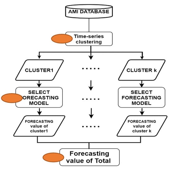
Figure 1.
Methodology for clustering of electricity demands for industrial areas. AMI, advanced metering infrastructure.
2.1. The Time-Series Clustering
2.1.1. Autocorrelation-Based Distances
Galeano et al. [35] suggested a clustering technique for autocorrelation function (ACF) in the time-series data. are estimated autocorrelation vectors of and , respectively, then and when . The ACF measures are expressed as below.
where is a weight matrix, and the equal weights are assumed by giving the initial as . In this case, becomes a Euclidiean distance measure between estimated ACF, as below.
The measure can be expressed as below as the considering geometric weights without time lag in ACF.
2.1.2. Normalized Periodogram-Based Distance
The periodogram distance proposed by Caiado et al. [36] is a metric to recognize the keyframes using a short boundary estimated on a sliding sub-window basis. If its correlation structure is more appropriate than the process scale, then it is better to use the normalized periodogram by using the Euclidean distance. The normalized periodogram measures are expressed as below.
where and are the periodograms of and , respectively. .
2.2. Forecasting Models
The double seasonal Holt–Winters (DSHW), trigonometric transform, Box–Cox transform, ARMA errors, trend and seasonal components (TBATS), fractional autoregressive integrated moving average (FARIMA), ARIMA with regression (Reg-ARIMA), and neural network nonlinear autoregressive (NN-AR) models are presented in this section.
2.2.1. The Double Seasonal Holt–Winters (DSHW) Method
The extension version for the double seasonal Holt–Winters method helped address multiple seasonal cycles, and can be written as below [37].
where represents the actual data; represent the seasonal component over time t (); and are the double seasonal cycles. The components and describe the level and trend of the series at time t, respectively. The coefficients are parameters for smoothing. is the forecasting value of h ahead of time t. The initial points are calculated as follows.
2.2.2. Trigonometric Transform, Box–Cox Transform, ARMA Errors, Trend and Seasonal Components (TBATS) Model
TBATS is an acronym for trigonometrical transformation, Box–Cox transformation, ARMA errors, trend and seasonal components. To overcome the problems of a wider seasonality and correlated errors in the exponential smoothing method, modified state-space models were introduced by De Livera et al. [38]. It is restricted to linear homoscedasticity, but the Box–Cox transformation can handle some types of non-linearity. This class of model is named BATS (Box–Cox transformation, ARMA errors, trend and seasonal components) and is defined as follows.
where is the Box–Cox transformed data for parameter at time t, depicts the local level, is the long-term trend, and is the short-term trend within the period of time. Rather than converging on zero, the value of finally meets on . is a damping parameter for the trend. is a series of ARMA models with orders (p, q) and is the white noise process with a mean of zero and a constant variance of . is the th seasonal cycle. , and are the smoothing parameters for .
The trigonometric seasonal approach incorporated into the model leads to a reduction in the estimation time (which increases with the number of parameters). This approach further accommodates non-integer seasonality. The final arguments for TBATS model () are explained with some additional equations, as below.
where is the number of harmonics for , which is a seasonal component. and are the smoothing parameters and . is the stochastic level of the th seasonal component by , and is the stochastic growth of the th seasonal component.
2.2.3. The Fractional Autoregressive Integrated Moving Average (FARIMA) Model
The FARIMA model is the common generalization of regular ARIMA processes when the degree of differencing d can take nonintegral values [39]. When the series follows ARIMA (p, d, q), the time series takes the following form:
where denotes the actual data observed at time t (), and describes the random errors assuming white noise on t with a mean of zero and a constant variance of . p and q are integers and orders in the model. , where p represents the degree of the autoregressive polynomial. , where q is the degree of the moving average polynomial. with , and .
2.2.4. Reg-ARIMA
The Reg-ARIMA model is proposed by Bell and Hilmer [40], it is a compound word of Regression and ARIMA. We consider hourly temperature data as a regressor, and double seasonality was fitted to explain the daily and weekly cycles. When the series follows ARIMA , the time series takes the following form:
where is a coefficient for the j-th regressor, denotes the actual data observed at time t (), and describes the random errors assuming white noise on t with a mean of zero and a constant variance of . p and q are integers and orders in the model. , where p represents the degree of the autoregressive polynomial. , where q is the degree of the moving average polynomial. Moreover, for the first seasonal operators, , and , where and are the degree of the first-seasonal autoregressive polynomial and moving average polynomial, respectively. For the second seasonal operators, , and , where and are the degree of the second-seasonal autoregressive polynomial and moving average polynomial, respectively., , and are the non-seasonal, first, and second seasonal difference operators of order d and D, respectively. and represent a seasonal cycle.
2.2.5. Neural Network Nonlinear Autoregressive (NN-AR)
Artificial neural network (ANN) models are designed similar to the neurons of a human brain. There are substantial complex forms of connected neurons in human brains. The network cells carry a specific signal from the body along an axon, transferring the signals to other neurons. The connections among axons are processed by a synapse. Some neurons are structured at birth, some grow and mature, and the rest die when considered to be non-useful. Likewise, the neural network model having a single-input neuron is defined below [41].
where p is an input, w is the weight of p, and b is a bias. f is a transfer function used to obtain an output of a, and it can be either linear or non-linear. If the neuron structure consists of R numbers of inputs as , the expression of summarized inputs can be expressed as follows:
where is the connection weight of the ith neuron from the jth neuron. n can also be expressed as a matrix form of inputs and weights: If there are S neurons in a layer, the model can be expressed as follows: where b is a bias vector, a is an output vector, and p is an input vector with the weight matrix, W. The matrix, W, can be written as follows:
If we expand the single layer to multiple layers, the output of the first layer can become an input to the next layer. For example, the output from the three layers can be explained as follows:
In this case, the third layer is considered as the output layer, and the first and second layers are hidden layers. The model is advantageous, because it can explain the complex relationships of the neurons with nonlinear functions. NN-AR models when additional exogenous variables are used for the ANN-based model.
3. Application of the Models
The auto-meter-reading (AMR) data obtained from Korea Electric Power Corporation (Naju, Korea) comprise data for 114 commercial buildings [42]. The data we provided were already refined; therefore, there was no extra step for data preprocessing. They were collected at 1 h intervals during the period from 12 February to 28 April 2014. A period of 10 weeks (10 February–20 April) was used for training, and the remaining one week (21 April–27 April) was used for testing. The datasets from the four weeks (24 March–20 April) prior to the test set were used for cluster analysis. Figure 2 shows an average time series profile of 114 buildings. The demand shows daily seasonal patterns, and there is a pattern of increasing demand from February to March.
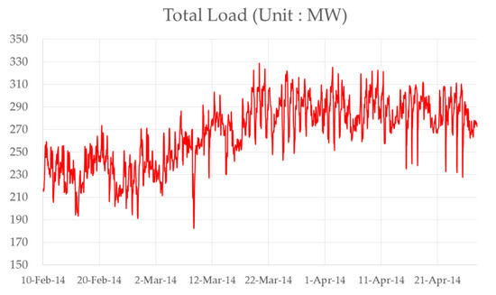
Figure 2.
Average demand plot from the 114 buildings.
We fitted the data with DSHW, TBATS, FARIMA, Reg-ARIMA, ANN, and NN-AR models; regarding the clustering, we chose the model showing the lowest mean absolute percentage error (MAPE) in each cluster. Then, the forecasting values from the aggregated and clustered data were compared. The model performances were evaluated using the mean absolute percentage error (MAPE). These evaluation methods are widely used to evaluate model performance, especially for STLF.
MAPE is defined as follows:
where is the actual value and is the forecasted demand at time t.
The number of clusters was chosen based on the silhouette metric. Figure 3 shows the time-series profiles of each of the 10 clusters measured. It demonstrates different patterns that have their own periodicity in the clusters. In this study, the double seasonality of daily and weekly patterns is considered. The optimal number of parameters at each k step in FARIMA models and Reg-ARIMA models was identified according to the corrected Akaike information criterion (AICc). Table 1 presents the FARIMA models in the training set of the aggregated data. The optimal parameter of d was selected as 0.1206 from the range (−0.5, 0.5), and then the number of p and q was selected as 5 and 5, respectively. Table 2 shows the identification of the best Reg-ARIMA models. Table 3 and Table 4 represent the hyperparameter tuning in ANN and NN-AR models, respectively. As we used nnetar function in the forecast package of R for the hyperparameter optimization in ANN and NN-AR models, we were able to search the number of nodes in the hidden layer, weight decay, iteration times, and network numbers. The optimized hyperparameters are chosen, indicating the minimum sum of squared errors.
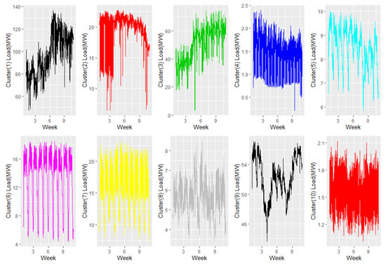
Figure 3.
Demand plot for 10 cluster groups by autocorrelation-based distances.

Table 1.
Identification of the best fractional autoregressive integrated moving average (FARIMA) model with . AICc, corrected Akaike information criterion.
Table 2.
Identification of the best regression ARIMA (Reg-ARIMA) model.
Table 3.
Hyperparameter optimization of the best artificial neural network (ANN) model.
Table 4.
Hyperparameter optimization of the best neural network nonlinear autoregressive (NN-AR) model.
Table 5, Table 6, Table 7 and Table 8 represent the estimated parameters and the results for assumptions in the training set. Figure 4 describes a dendrogram from the autocorrelation-based distances clustering. Table 9 presents the results of the MAPE in the test set and the number observations assigned in each cluster. It shows that the TBATS model is superior to other models in clusters 5 and 9 and the DSHW model elicits high accuracy in cluster 6. For clusters 1, 2, 3, 4, 7, 8, and 10, NN-AR was the most suitable model. Therefore, each cluster yields forecasting values from the different models. Further, we fit the NN-AR model for the aggregated data because it was superior to the other models in the dataset. Consequently, a week long forecasting was conducted for each cluster and total usage. In Table 10, the results indicate the MAPE of the aggregated forecasting value and the total usage data for the forecasted amounts for each cluster through the cluster analysis method. The MAPE for the forecasting of total data by the NN-AR model is 3.86%. The MAPE for the forecasting of aggregated data by clustering of autocorrelation-based distances is 3.32%, which is the summation forecasting result based on cluster-specific forecasting; the result based on clustering of normalized periodogram-based distance is 3.94%; the forecasting through clustering of autocorrelation-based distances showed a more accurate overall forecasting.
Table 5.
Parameter estimations of double seasonal Holt–Winters (DSHW).
Table 6.
Parameter estimations of the TBATS model.
Table 7.
Parameter estimations of the FARIMA model.
Table 8.
Parameter estimations of the Reg-ARIMA model.
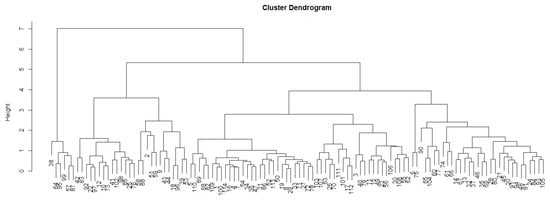
Figure 4.
Dendrogram for autocorrelation-based clustering.
Table 9.
Mean absolute percentage error (MAPE) of training dataset by autocorrelation-based distances clustering approach.
Table 10.
Result of forecasting accuracy by MAPE.
4. Conclusions
It is well known that forecasts based on the bottom-up method are more accurate than forecasts based on the top-down method if companies’ power demand pattern is constant. However, in the actual operating establishment, as each company’s prediction can cause problems such as excessive computing time, it is necessary to determine the most appropriate method.
This study presents a bottom-up power prediction method through the results of a cluster analysis of electricity demand for each company in a smart grid environment. To this end, data from 114 companies recorded using auto-metering-reading (AMR) devices were classified into 10 clusters using time series cluster analysis. Owing to the strong time-series characteristics of power demand, this study uses clustering of autocorrelation-based distances and normalized periodogram distance. The power demand classified through time-series cluster analysis revealed different patterns according to the characteristics of the companies. As the demand pattern for each cluster was different, the optimal forecasting model for each cluster was selected using the NN-AR and TBATS models. Finally, the total power demand was calculated based on the aggregated forecasting results for each cluster.
The forecasting result using the time-series cluster (autocorrelation-based distances) analysis of the bottom-up method was superior to that of the top-down method by about 0.5%.
This study proposed a solution to the problem of low predictive accuracy and computing speed owing to big data management in the process of transitioning to the smart grid method. If the power consumption of all companies is forecasting, accuracy will increase, but the program run time will be longer. In addition, if all companies and households with electricity demand are considered, the electricity demand forecasting will take longer. Accordingly, in real-time operations, it is proposed to improve the accuracy of prediction through time-series cluster analysis and to reduce the program run time by predicting each cluster analysis result. This method is proposed as a proactive response to issues related to the smart grid method with regard to national power management.
The results of this study may be relevant only to the demand data of generic companies. Therefore, any future analysis based on cluster characteristics may consider specificities. Future studies should examine the patterns of demand based on company characteristics by analyzing corporate information. Further, demand patterns should be examined according to the characteristics of the company’s industry, and researchers should determine the optimal model for each cluster characteristic. Finally, it is necessary to determine a system automation method that can be used in an actual power operation establishment.
Author Contributions
Conceptualization, H.-g.S. and S.K.; Software, Y.K.; Formal Analysis, H.-g.S.; Formal Analysis, H.-g.S. and S.K.; Investigation, Y.K.; Project administration, S.K.; Supervision, S.K.; Writing—original draft, H.-g.S.; Writing—review & editing, Y.K.; Visualization, H.-g.S. All authors have read and agreed to the published version of the manuscript.
Funding
This research was funded by the National Research Foundation of Korea grant number 2016R1D1A1B01014954.
Acknowledgments
The authors are appreciative of the worthy commentaries and advice from the respected reviewers. Their helpful remarks have improved the power and importance of our paper.
Conflicts of Interest
The authors declare no conflict of interest.
References
- Huang, A.Q. Power semiconductor devices for smart grid and renewable energy systems. In Power Electronics in Renewable Energy Systems and Smart Grid; Wiley: Hoboken, NJ, USA, 2019; pp. 85–152. [Google Scholar]
- Korea Power Exchange. Available online: http://www.kpx.or.kr (accessed on 9 May 2020).
- Renn, O.; Marshall, J.P. Coal, nuclear and renewable energy policies in Germany: From the 1950s to the “Energiewende”. Energy Policy 2016, 99, 224–232. [Google Scholar] [CrossRef]
- Reyna, J.; Chester, M.V. Energy efficiency to reduce residential electricity and natural gas use under climate change. Nat. Commun. 2017, 8, 14916. [Google Scholar] [CrossRef]
- Alberg, D.; Last, M. Short-term load forecasting in smart meters with sliding window-based ARIMA algorithms. Vietnam. J. Comput. Sci. 2018, 5, 241–249. [Google Scholar] [CrossRef]
- Nie, H.; Liu, G.; Liu, X.; Wang, Y. Hybrid of ARIMA and SVMs for Short-Term Load Forecasting. Energy Procedia 2012, 16, 1455–1460. [Google Scholar] [CrossRef]
- Sigauke, C.; Chikobvu, D. Prediction of daily peak electricity demand in South Africa using volatility forecasting models. Energy Econ. 2011, 33, 882–888. [Google Scholar] [CrossRef]
- Kim, Y.; Son, H.-G.; Kim, S. Short term electricity load forecasting for institutional buildings. Energy Rep. 2019, 5, 1270–1280. [Google Scholar] [CrossRef]
- Chan, K.Y.; Dillon, T.S.; Singh, J.; Chang, E. Neural-Network-Based Models for Short-Term Traffic Flow Forecasting Using a Hybrid Exponential Smoothing and Levenberg–Marquardt Algorithm. IEEE Trans. Intell. Transp. Syst. 2011, 13, 644–654. [Google Scholar] [CrossRef]
- Sohn, H.-G.; Jung, S.-W.; Kim, S. A study on electricity demand forecasting based on time series clustering in smart grid. J. Appl. Stat. 2016, 29, 193–203. [Google Scholar] [CrossRef]
- Brożyna, J.; Mentel, G.; Szetela, B.; Strielkowski, W. Multi-Seasonality in the TBATS Model Using Demand for Electric Energy as a Case Study. Econ. Comput. Econ. Cybern. Stud. Res. 2018, 52, 229–246. [Google Scholar] [CrossRef]
- Dudek, G. Pattern-based local linear regression models for short-term load forecasting. Electr. Power Syst. Res. 2016, 130, 139–147. [Google Scholar] [CrossRef]
- Cao, G.; Wu, L.-J. Support vector regression with fruit fly optimization algorithm for seasonal electricity consumption forecasting. Energy 2016, 115, 734–745. [Google Scholar] [CrossRef]
- Barman, M.; Choudhury, N.D.; Sutradhar, S. A regional hybrid GOA-SVM model based on similar day approach for short-term load forecasting in Assam, India. Energy 2018, 145, 710–720. [Google Scholar] [CrossRef]
- Bin Song, K.; Baek, Y.-S.; Hong, D.H.; Jang, G. Short-Term Load Forecasting for the Holidays Using Fuzzy Linear Regression Method. IEEE Trans. Power Syst. 2005, 20, 96–101. [Google Scholar] [CrossRef]
- Sadaei, H.J.; Guimarães, F.G.; Da Silva, C.J.; Lee, M.H.; Eslami, T. Short-term load forecasting method based on fuzzy time series, seasonality and long memory process. Int. J. Approx. Reason. 2017, 83, 196–217. [Google Scholar] [CrossRef]
- Zheng, Z.; Chen, H.; Luo, X. A Kalman filter-based bottom-up approach for household short-term load forecast. Appl. Energy 2019, 250, 882–894. [Google Scholar] [CrossRef]
- Dong, X.; Qian, L.; Huang, L. Short-term load forecasting in smart grid: A combined CNN and K-means clustering approach. In Proceedings of the 2017 IEEE International Conference on Big Data and Smart Computing (BigComp), Jeju Island, Korea, 13–16 February 2017. [Google Scholar]
- Khan, S.; Javaid, N.; Chand, A.; Khan, A.B.M.; Rashid, F.; Afridi, I.U. Electricity load forecasting for each day of week using deep CNN. In Proceedings of the Workshops of the International Conference on Advanced Information Networking and Applications; Springer: Berlin/Heidelberg, Germany, 2019. [Google Scholar] [CrossRef]
- Shi, H.; Xu, M.; Li, R. Deep Learning for Household Load Forecasting—A Novel Pooling Deep RNN. IEEE Trans. Smart Grid 2017, 9, 5271–5280. [Google Scholar] [CrossRef]
- Yang, L.; Yang, H. Analysis of Different Neural Networks and a New Architecture for Short-Term Load Forecasting. Energies 2019, 12, 1433. [Google Scholar] [CrossRef]
- Zheng, H.; Yuan, J.; Chen, L. Short-Term Load Forecasting Using EMD-LSTM Neural Networks with a Xgboost Algorithm for Feature Importance Evaluation. Energies 2017, 10, 1168. [Google Scholar] [CrossRef]
- Bouktif, S.; Fiaz, A.; Ouni, A.; Serhani, M.A. Optimal Deep Learning LSTM Model for Electric Load Forecasting using Feature Selection and Genetic Algorithm: Comparison with Machine Learning Approaches. Energies 2018, 11, 1636. [Google Scholar] [CrossRef]
- Mohammadi, M.; Talebpour, F.; Safaee, E.; Ghadimi, N.; Abedinia, O. Small-Scale Building Load Forecast based on Hybrid Forecast Engine. Neural Process. Lett. 2017, 48, 329–351. [Google Scholar] [CrossRef]
- Ghadimi, N.; Akbarimajd, A.; Shayeghi, H.; Abedinia, O. A new prediction model based on multi-block forecast engine in smart grid. J. Ambient. Intell. Humaniz. Comput. 2017, 9, 1873–1888. [Google Scholar] [CrossRef]
- Kim, N.; Kim, M.; Choi, J.K. Lstm based short-term electricity consumption forecast with daily load profile sequences. In Proceedings of the 2018 IEEE 7th Global Conference on Consumer Electronics (GCCE), Nara, Japan, 9–12 October 2018. [Google Scholar]
- Vrablecová, P.; Ezzeddine, A.B.; Rozinajová, V.; Šárik, S.; Sangaiah, A.K. Smart grid load forecasting using online support vector regression. Comput. Electr. Eng. 2018, 65, 102–117. [Google Scholar] [CrossRef]
- Chou, J.-S.; Hsu, S.-C.; Ngo, N.-T.; Lin, C.-W.; Tsui, C.-C. Hybrid Machine Learning System to Forecast Electricity Consumption of Smart Grid-Based Air Conditioners. IEEE Syst. J. 2019, 13, 3120–3128. [Google Scholar] [CrossRef]
- Mohammad, R. AMI Smart Meter Big Data Analytics for Time Series of Electricity Consumption. In Proceedings of the 2018 17th IEEE International Conference on Trust, Security and Privacy in Computing And Communications/12th IEEE International Conference On Big Data Science And Engineering (TrustCom/BigDataSE), New York, NY, USA, 1–3 August 2018. [Google Scholar]
- Muralitharan, K.; Sakthivel, R.; Vishnuvarthan, R. Neural network based optimization approach for energy demand prediction in smart grid. Neurocomputing 2018, 273, 199–208. [Google Scholar] [CrossRef]
- Kundu, S.; Ramachandran, T.; Chen, Y.; Vrabie, D. Optimal Energy Consumption Forecast for Grid Responsive Buildings: A Sensitivity Analysis. In Proceedings of the 2018 IEEE Conference on Control Technology and Applications (CCTA), Copenhagen, Denmark, 21–24 August 2018. [Google Scholar]
- Ahmad, A.; Javaid, N.; Mateen, A.; Awais, M.; Khan, Z.A. Short-Term Load Forecasting in Smart Grids: An Intelligent Modular Approach. Energies 2019, 12, 164. [Google Scholar] [CrossRef]
- Amin, P.; Cherkasova, L.; Aitken, R.; Kache, V. Automating energy demand modeling and forecasting using smart meter data. In Proceedings of the 2019 IEEE International Congress on Internet of Things (ICIOT), Milan, Italy, 8–13 July 2019. [Google Scholar]
- Motlagh, O.; Berry, A.; O’Neil, L. Clustering of residential electricity customers using load time series. Appl. Energy 2019, 237, 11–24. [Google Scholar] [CrossRef]
- Galeano, P.; Peña, D. Multivariate Analysis in Vector Time Series; Universidad Carlos III de Madrid: Madrid, Spain, 2001. [Google Scholar]
- Caiado, J.; Crato, N.; Peña, D. A periodogram-based metric for time series classification. Comput. Stat. Data Anal. 2006, 50, 2668–2684. [Google Scholar] [CrossRef]
- Taylor, J.W. Triple seasonal methods for short-term electricity demand forecasting. Eur. J. Oper. Res. 2010, 204, 139–152. [Google Scholar] [CrossRef]
- De Livera, A.M.; Hyndman, R.J.; Snyder, R.D. Forecasting Time Series With Complex Seasonal Patterns Using Exponential Smoothing. J. Am. Stat. Assoc. 2011, 106, 1513–1527. [Google Scholar] [CrossRef]
- Shu, Y.; Jin, Z.; Zhang, L.; Wang, L.; Yang, O.W. Traffic prediction using FARIMA models. In Proceedings of the 1999 IEEE International Conference on Communications (Cat. No. 99CH36311), Vancouver, BC, Canada, 6–10 June 1999. [Google Scholar]
- Bell, R.W.; Hillmer, S.C. Modeling time series with calendar variation. J. Am. Stat. Assoc. 1983, 78, 526–534. [Google Scholar] [CrossRef]
- Beale, H.D.; Demuth, H.B.; Hagan, M.T. Neural Network Design, Martin Hagan; Pws: Boston, MA, USA, 2014. [Google Scholar]
- Korea Electric Power Corporation. Available online: http://www.kepco.co.kr (accessed on 9 May 2020).


© 2020 by the authors. Licensee MDPI, Basel, Switzerland. This article is an open access article distributed under the terms and conditions of the Creative Commons Attribution (CC BY) license (http://creativecommons.org/licenses/by/4.0/).