Control Strategy for Helicopter Thermal Management System Based on Liquid Cooling and Vapor Compression Refrigeration

Abstract

With the continuous application of high-power electronic equipment in aircraft, highly efficient heat transfer technology has been emphasized for airborne applications. In this paper, a thermal management system based on an antifreeze liquid cooling loop and a vapor compression refrigeration loop is presented for high-power airborne equipment in a helicopter. The simulation models of the thermal management system are built in order to study its control strategy for the changing flight conditions. The antifreeze-refrigerant evaporator and air-refrigerant condenser are specially validated with the experimental data. A dual feedforward proportion integration differentiation and expert control algorithm are adopted in the inlet temperature of the cold plate and sub-cooling control of the refrigerant by regulating the compressor speed and the fan speed, respectively. A preheating strategy for antifreeze is set up to decrease its flow resistance in cold day conditions. The control strategy for the thermal management system is finally built based on the above control methods. In this paper, two extreme conditions are discussed, including cold and hot days. Both the simulation results show that the superheated, sub-cooling and antifreeze inlet temperature of the cold plate can be controlled at 3 to8 °C, −10 to −3 °C and 18 to22 °C, respectively. Under the same changing flight envelope, the coefficient of performance of the vapor compression refrigeration loop is relatively stable on the cold day, which is about 6, while it has a range of 2.58–4.9 on the hot day.

1. Introduction

Various advanced electronic equipment have been applied in military helicopters in order to improve their comprehensive performance. The usage of high-energy electronic equipment has also brought a continuous increase in heat load, which is a huge challenge for the environmental control system (ECS). For the cooling of the electronic equipment, the active methods that require energy or a generator, such as a pump, are widely applied in aircraft and military helicopters, such as an air cycle cooling (ACR) system and a vapor compression refrigeration (VCR) system. However, dissipation of this huge heat load by a conventional ACR system increases the engine bleed air consumption and may have a negative impact on engine performance. Hence, highly efficient heat management technology with a VCR system may be adopted in future helicopters, such as liquid cooling, microchannel cooling, etc.

Sarafraz and Arjomandi pointed out that microchannel heat exchanging systems are relatively new instruments and can transfer significant amounts of heat in a small space, and they investigated the thermal performance and pressure drop of a microchannel heat sink at high-temperatures [1]. Compared to the embedded high thermal conductivity at the same thermal conductivity ratio, Dadsetani et al. pointed out that the hybrid method can reduce the maximum disk temperature up to 90% [2]. Some advanced efficient heat transfer technologies for electronic equipment have been studied [3,4,5,6]. Moreover, the corresponding control research should be carried out for the VCR system.

Deymi-Dashtebayaz et al. [7] investigated the impact of various refrigerants on the efficiency of the geothermal heat pump operation. The critical parameters such as coefficient of performance (COP), exergy efficiency and exergy destruction for various components were calculated and investigated.

Michalak pointed out that high-performance military aircraft should use a VCR system instead of a direct air refrigeration system [8]. He conducted experiments with two control strategies for a vapor loop system. The experimental results showed that their method could control electronic expansion valve (EEV) opening very well. Military aircraft and helicopters can gain improved performance and efficiency through the aircraft thermal management systems by the incorporation of VCR systems in place of standard air loop systems [9,10,11,12,13]. The VCR system has been applied in civil areas. However, in the aviation field, the heat loads often are large and time-varying. In addition, the heat sink often varies with the flight height over a short period [14,15,16,17].

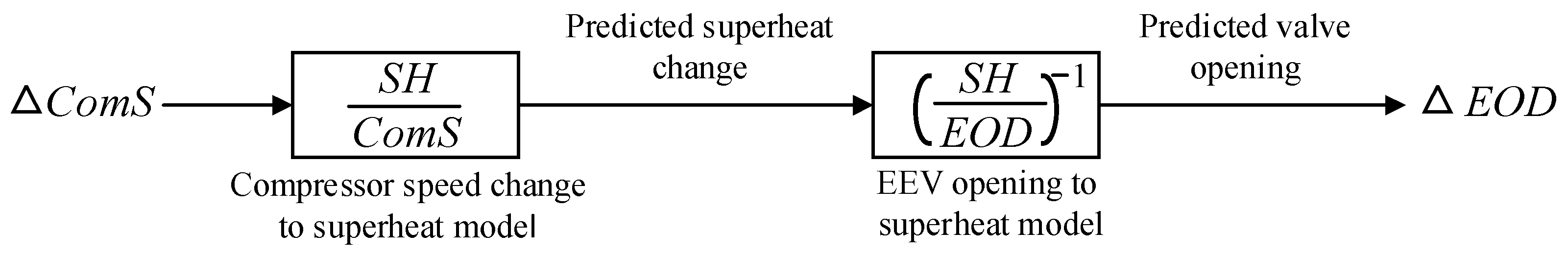
A dual single input–single output (SISO) control strategy was developed by Marcinichen based on the proportion integration feedback method [18]. It used a variable opening expansion valve and a variable speed compressor to adjust refrigerant valve position and compressor speed, respectively. Correspondingly, its refrigerant flow rate and evaporator superheat had to be adjusted by a variable speed compressor and a variable opening expansion valve, respectively. The SISO control strategy can control evaporator superheating and cooling capacity in good working states.

Rasmussen and Alleyne created a control-oriented model that balanced simplicity with accuracy and developed a gain-scheduled multiple input – multiple output (MIMO) feedback control strategy for a refrigeration and air-conditioning system [19,20]. Their results demonstrated that the gain-scheduled approach extended advantages over the entire operating system compared to linear control techniques. Elliott and Rasmussen proposed a cascaded control scheme only requiring evaporator pressure and temperature as measured values, and only handling the opening of the expansion valve with cascaded control [21]. Their control method had better performance than the complex non-linear or gain-scheduled controllers.

It is well known that the heat exchangers used in VCR typically operate with multiple and non-linear fluid phases [22,23,24,25]. In order to cope with inherent complexity and nonlinearity in VCR systems, Li et al. dealt with an empirical dynamic model based on experimental data and presented a decoupling control of the VCR [22]. Their experiment and simulation results indicated that the proposed model could describe the actual system. On the basis of the empirical model, Li designed a PI controller scheme with a decoupling model to manage the thermal capacity and superheating independently [26]. Their works are both effective and exhibit high performance.

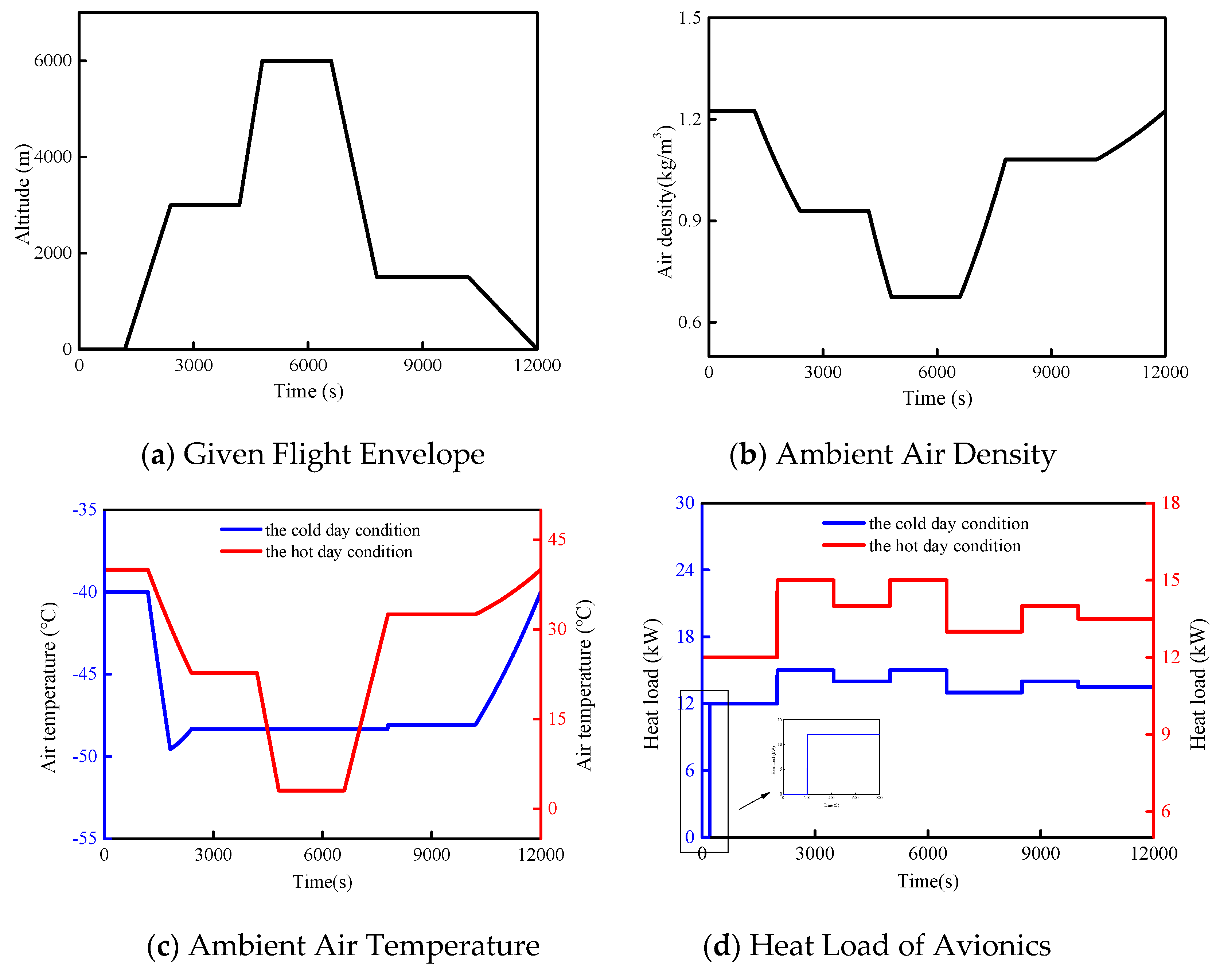
The requirement for future advanced aircraft is the need for precise temperature control of time-varying loads and flight environments. The VCR can offer higher coefficient of performance (COP) and has some advantages in weight, cost and volume than the air loop system. However, there are some challenges for the design of VCR control for advanced helicopters. Firstly, the advanced helicopter requires precise temperature control for rapidly changing heat loads. Secondly, the working environment of advanced helicopters is very extreme, so that the heat sink varies widely in a short period. For example, the air temperature may be over 40 °C on the ground and −20 °C at high altitude in summer. Thirdly, advanced aircraft carry out tasks under various weather conditions, including standard day, cold day and hot day. In extremely cold environment conditions, liquid in the coolant loop should be preheated. All in all, there are some challenges for research of VCR for advanced helicopters.

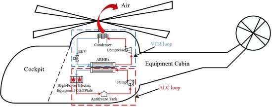
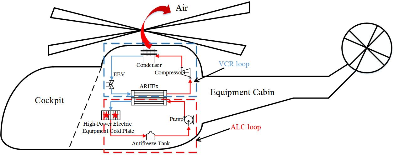
It has be seen from the previous results that various methods have been studied by many researchers. However, few studies have been conducted on extreme conditions, such as extreme hot weather and extreme cold weather [27,28,29]. In this paper, a helicopter thermal management system (TMS) based on antifreeze liquid cooling (ALC) and VCR loops is presented. Its control strategy for various weather is further studied in order to ensure the environmental adaptability of the helicopter TMS.

2. System Description of the Helicopter TMS

2.1. System Configuration

During a helicopter flight process, its external environment is complex and changeable. The change ranges of temperature and pressure are −40 to 40 °C and 0.4 to 1 bar, respectively. Hence, ram air as the cooling source of helicopter TMS is always in a time-varying state, which leads to instability of the heat exchange process in the VCR. Meanwhile, the heat flux of avionics increases continuously. This means that the ram air cooling in common use cannot meet the temperature control requirement at all for high power helicopters. Instead, liquid cooling has been of interest because of its high heat transfer coefficient and working stability. In order to meet the control requirement of helicopter high-power avionics under various conditions, this paper proposes a helicopter TMS based on ALC and VCR loops.

The helicopter TMS is composed of the VCR loop with R134a working fluid, the ALC loop and its control unit. The ALC and VCR loops are coupled together through the antifreeze–refrigerant heat exchanger (ARHEx). The ALC loop absorbs the large amount of heat dissipated from the high-power electronic equipment and transfers the waste heat to the VCR loop through the antifreeze–refrigerant evaporator. The VCR loop finally transfers the waste heat to the outside ram air effectively. The system configuration is shown in Figure 1.

2.2. Requirements and Control Strategy

2.2.1. Control Requirement

According to the working principle of the helicopter TMS as shown in Figure 1, its control objectives include the superheating (SH), the sub-cooling (SC) and the inlet temperature of the cold plate (T_cp,in). The best operating temperature range of airborne electronic equipment is 15–25 °C. Some ground experiments were completed for this thermal management system. The experimental data show that the system is stable when the range of superheating is from 3–8 °C and the range of sub-cooling is from −10 to −3 °C. Due to the different control methods of antifreeze inlet temperature of the cold plate, superheating and sub-cooling, different control requirements are obtained for each target, as shown in

Table 1. Control requirements.

No.	Symbol	Value	Unit
1	Tcp,in	20 ± 2	°C
2	SH	5 ± 1	°C
3	SC	[−10,3]	°C

.

2.2.2. Couple Control Method of SH and T_cp,in

The refrigerant superheating at the evaporator outlet is expressed as follows:

$$SH=T_{eva,out}-T_{eva}$$

(1)

where T_eva,out is the refrigerant outlet temperature of the evaporator in °C; T_eva is the evaporation temperature in °C.

Due to the coupling relationship between SH and T_cp,in, it is hard to satisfy the control requirement just using a simple proportion integration differentiation (PID) control algorithm. According to the principle of heat transfer function and feed-forward control structure [30,31], two compensators are introduced for the helicopter TMS in consideration of the effects of the change of EEV opening degree (EOD) on T_cp,in and the change of compressor speed (ComS) on SH, respectively. T_cp,in,set and SH_set are the set values of T_cp,in and SH, respectively. △EOD and △ComS are the variation values. ComS has influence on SH and T_cp,in, but the change of T_cp,in has a certain delay compared with the response speed of SH. The control structure is shown in Figure 2 [31].

The influence of EOD on Tcp,in is limited and can be ignored, so only compensator, G_ComS,SH, needs to be calculated. The control structure is shown in Figure 3 [11].

With reference to previous research [11,30,31], the transfer functions between SH and T_cp,in can be expressed by the following equations:

$$\frac{SH}{ComS}=\frac{k_1{e}^{-T{d}_{1}t}}{T{p}_{1}t+1}$$

(2)

$$\frac{SH}{EOD}=\frac{k_2{e}^{-T{d}_{2}t}}{T{p}_{2}t+1}$$

(3)

where k is the coupling coefficient; Td is the time delay in s; Tp is the time constant in s; t is the time variable in s; the subscript 1 indicates the relationship between the SH and ComS; the subscript 2 indicates the relationship between the SH and EOD.

A series of step response simulations were conducted to identify the parameters in Equations (3) and (4). The simulation results were identified with the MATLAB toolbox “system identification” [31]. Some results of the parameters in Equations (3) and (4) are shown in

Table 2. Partial values of k, Td and T_p.

Change Parameter	Change Value	Change Range	k1	Td1	Tp1
Step change of EOD	ComS = 5000 RPM	66–67%	0.76955	1.568	7.3
		67–68%	0.99066	1.867	6.9
		68–69%	1.3636	2.592	6.6
	ComS = 5100 RPM	66–67%	0.79464	1.158	8.3
		67–68%	1.0334	1.363	9.6
		68–69%	1.4519	2.322	7.3
Change Parameter	Change Value	Change Range	k2	Td2	Tp2
Step change of ComS	EOD = 68%	5000–5050	1.2318	0.485	8.7
		5050–5100	1.2953	0.682	7.6
		5100–5150	1.3615	0.953	10.1
	EOD = 69%	5000–5050	0.85841	0.69	9.5
		5050–5100	0.8906	0.543	8.4
		5100–5150	0.92329	0.529	5.2

. The time delays, Td1 and Td2, are very close to each other and can be ignored. The time constants, T_p1 and T_p2, in the transfer function are on the same order of magnitude approximately (8 s). Therefore, in order to reduce the complexity of the compensator, it is necessary to compensate the time constant. Therefore, the feedforward compensation can be simplified using Equation (5).

$$G_{C\mathrm{oms},SH}=\frac{SH}{ComS}{\left(\frac{SH}{EOD}\right)}^{-1}$$

(4)

2.2.3. Control Method of SC

The refrigerant sub-cooling at the condenser outlet is expressed as:

$$SC=T_{con,out}-T_{con}$$

(5)

where T_con,out is the refrigerant outlet temperature of the condenser in °C; T_con is the condensation temperature in °C.

The heat in the R134a loop can be transferred to the external ram air. The SC control is realized by adjusting the air speed of the condenser fan, which is determined according to the ground steady-state experiment results. The control range of SC is usually between −10 °C and −3 °C. The air speed of the fan varies with the ground ambient temperature, as shown in

Table 3. Steady-state experimental of SC.

Ground Ambient Temperature	Air Speed (m/s)	SC (°C)
−40 °C ≤ T0 < 0 °C	1 m/s	[−10,−3]
0 °C ≤ T0 < 10 °C	2 m/s	[−10,−3]
10 °C ≤ T0 < 25 °C	3 m/s	[−10,−3]
25 °C ≤ T0 < 35 °C	4 m/s	[−10,−3]
35 °C ≤ T0 ≤ 40 °C	5 m/s	[−10,−3]

. The relationship between the SC of condenser and the air speed of the fan is obtained based on the ground test data. The boundary conditions in the ground steady-state experiment were as follows: the range of ground ambient temperature was −40–40 °C, the range of pressure was 0.5–1 bar and the range of heat load was 10–20 kW.

2.2.4. Antifreeze Preheat Method

The antifreeze fluid is 65% ethylene glycol solution, in the ALC loop, and its freezing point is −65 °C. The fluid temperature greatly affects the antifreeze kinematic viscosity. In some extreme cold day conditions, the ground ambient temperature may reach −40 °C, which will badly lead to the increase of the flow resistance of the antifreeze in the ALC loop.

The relationship of the antifreeze temperature, the kinematic viscosity and the pump power consumption is shown in Figure 4. When the antifreeze temperatures are −40 °C, 0 °C, 5 °C and 10 °C, the pump power consumptions are 26.5 kW, 2.6 kW, 2.12 kW and 1.99 kW, respectively. The pump power is reduced more than 10 times. When the temperature reaches 5 °C, the kinematic viscosity does not decrease anymore, and the heat transfer efficiency does not increase very much. Considering the temperature requirement of electronic equipment, the preheated temperature of antifreeze is finally set at 5 °C.

The antifreeze is heated by a 5 kW heating device in the tank; the simulation results showed that the heating time required from −40 °C to 5 °C was 136 s.

2.2.5. Control Strategy of the Helicopter TMS

The control strategy of the helicopter TMS is shown in Figure 5, in which T₀ is the ground temperature, and T_tank is the temperature of the antifreeze tank. E11, E13, E2 and E5 are explained in Figure 1.

The working principle of the control strategy is as follows:

• Cold day condition (−40 °C ≤ T_tank < 5 °C)
  A cold day condition is defined as −40 °C ≤ T_tank < 5 °C, where T_tank is the temperature of the antifreeze tank. In the cold day condition, the heat transfer efficiency of system is low, and the antifreeze should be preheated by an electric heater, E11. The preheating process is over when T_tank is larger than 5 °C, and E11 is powered off. The antifreeze is driven to circulate in the ALC loop by a pump, E13, which also leads the antifreeze temperature to rise. The next logical step is to start the VCR loop by powering on E2 and E5 after 10 s. Only after the helicopter TMS has worked normally can the avionics be loaded.
• Hot day condition
  When the system is not in a cold day condition, the antifreeze is directly driven to circulate in the ALC loop by the pump, E13. After 10 s, the VCR starts. Only after the helicopter TMS works normally can the heat of avionics be loaded.

3. Mathematical Model

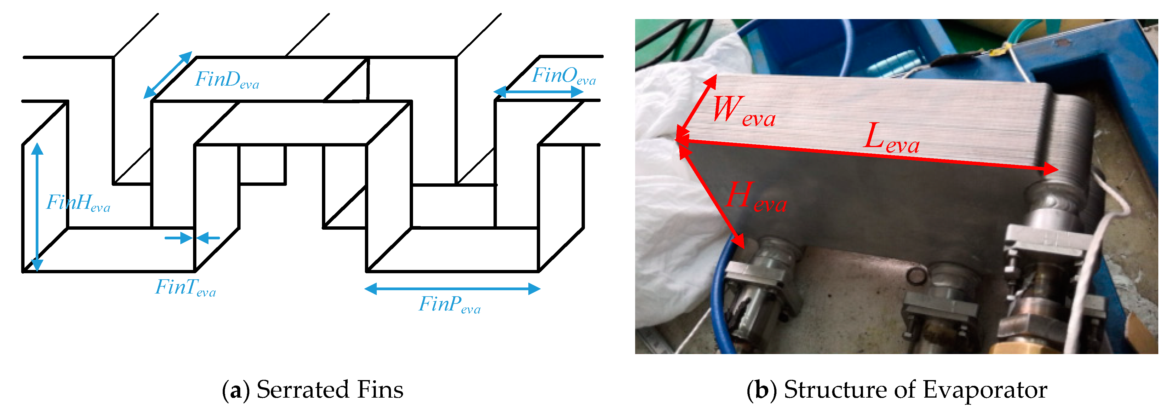
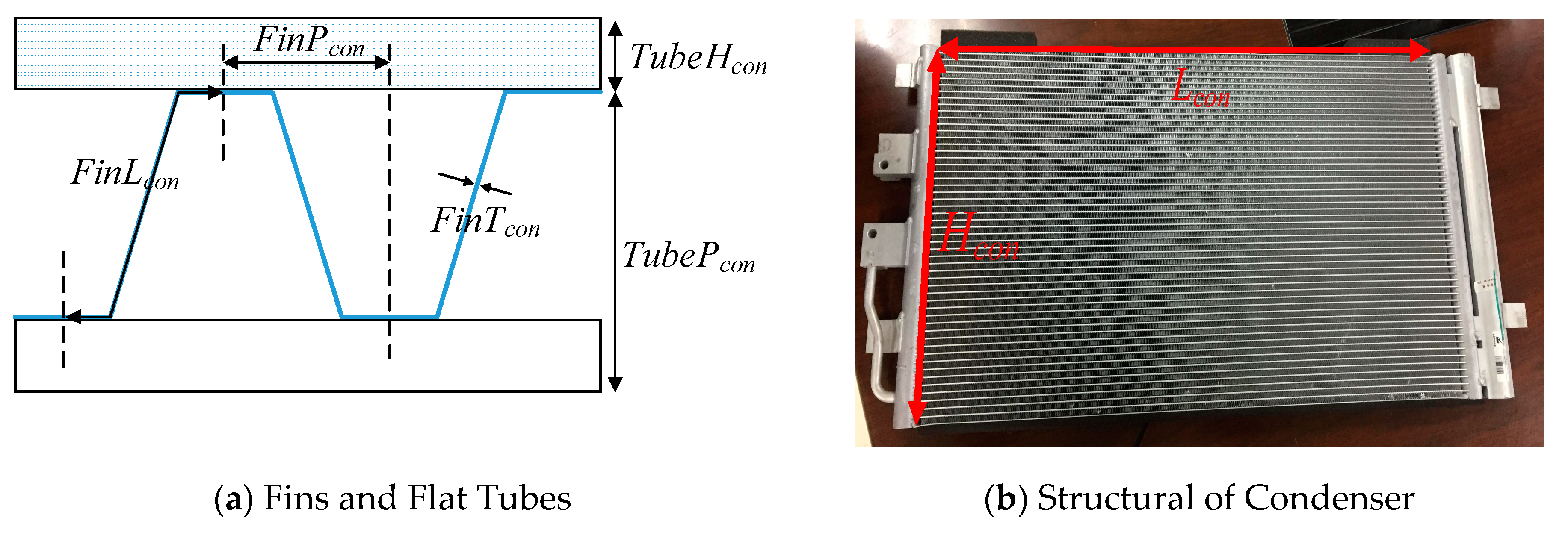
In the helicopter TMS, the condenser is a parallel flow air-cooled heat exchanger, and the evaporator is a plate-fin antifreeze-R134a heat exchanger.

The fundamental assumptions [32,33] for homogeneous flow model are as follows:

• No slip between the two phases;
• Thermodynamic equilibrium between the phases;
• No non-condensable gas in the phase transformation process of refrigerant;
• One-dimensional steady-state flow of the flow of the refrigerant in the flat tube.

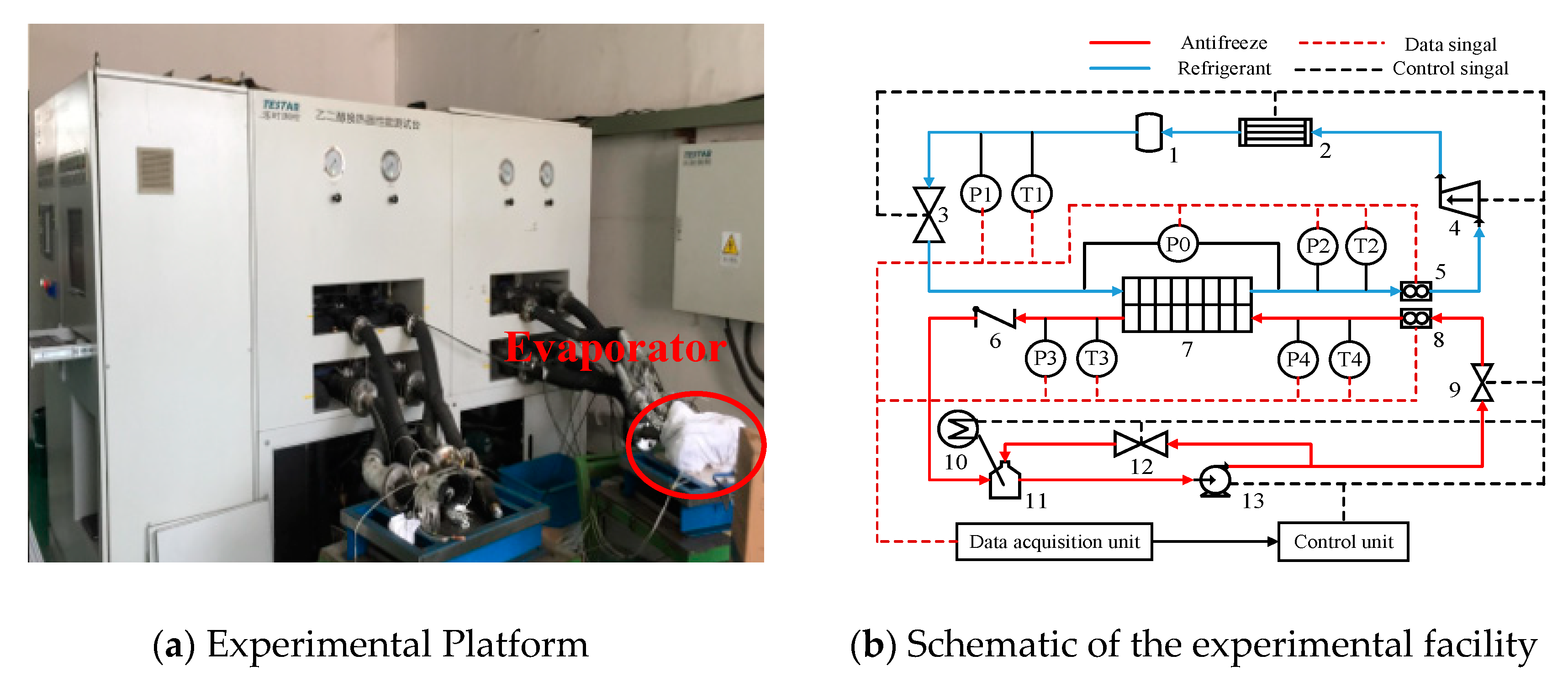
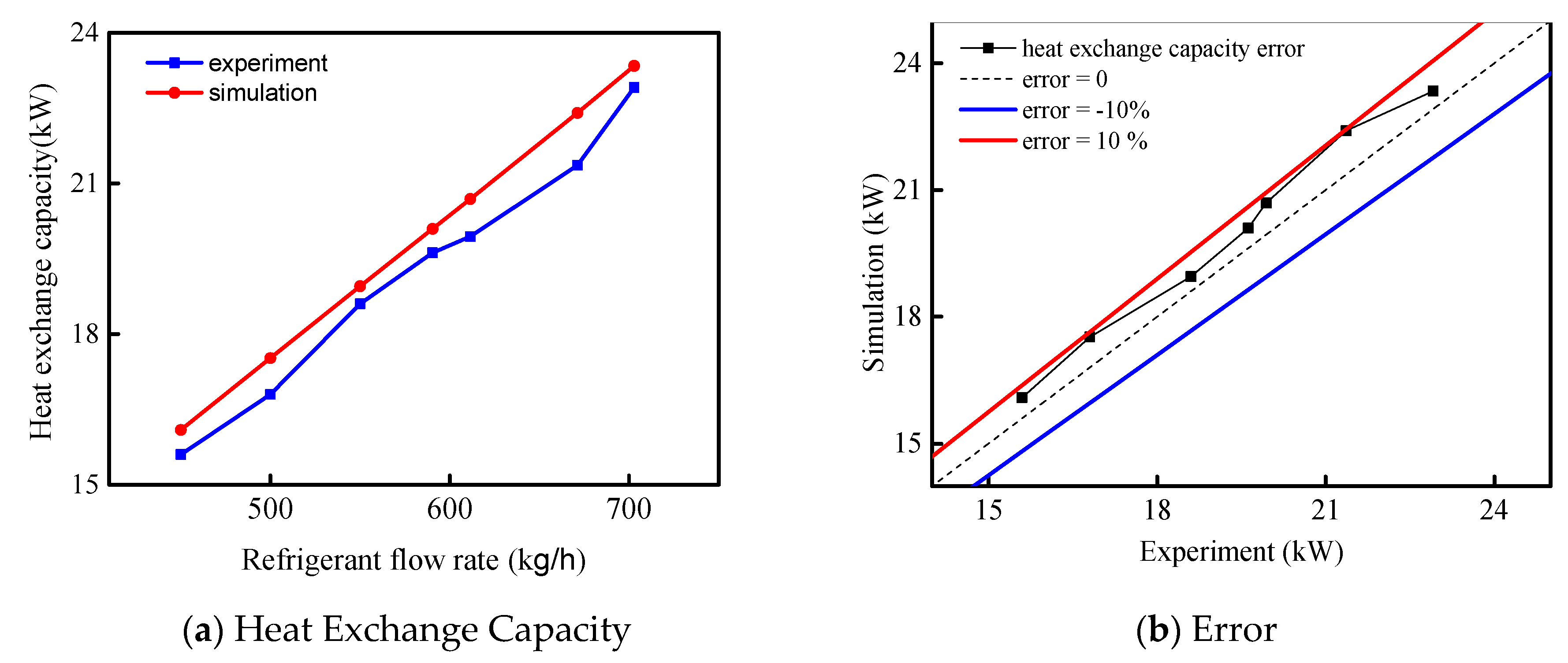
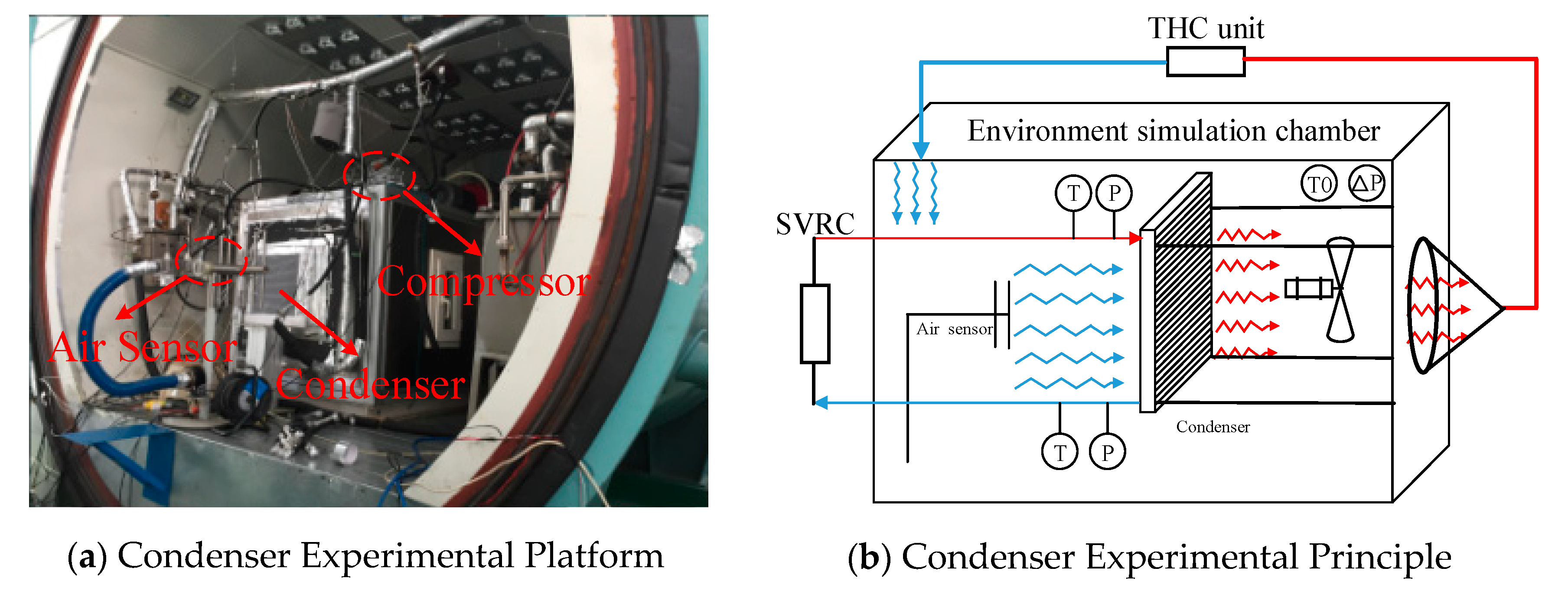
The steady-state experimental correction of evaporator and condenser was carried out using the homogeneous flow model. A homogenous flow model was validated by experimental results for an evaporator [34]. About 92% of deviations between predicted and tested pressure drops were within ±20%.

The components of the TMS mainly include a antifreeze–refrigerant heat exchanger (ARHEx), an air-R134a heat exchanger, an expansion valve and a compressor. These calculation models are established in this section.

3.1. Evaporator

3.1.1. R134a Side of the Evaporator

The transient thermal equation of the R134a is established in Equation (6), and the average temperature of the R134a can be calculated by the following equation [35].

$$\begin{array}{ll}{m}_{eva,R}{c}_v\frac{d{T}_{eva,R,ref}}{dt}& =E_{eva,R}\left(T_{eva,R,in}-T_{wall}\right)\\ & +\left({\dot{m}}_{eva,R,in}\cdot h_{eva,R,in}-{\dot{m}}_{eva,R,out}\cdot h_{eva,R,out}\right)\end{array}$$

(6)

where m_eva,R and c_v are the mass (kg) and specific heat of the R134a (J/(kg·°C)), respectively; T_eva,R,in and 1/E_eva,R are the temperatures of the inner wall (°C) and the thermal resistance of the convection between the inner wall and the R134a inside the evaporator (W/°C), respectively; ${\dot{m}}_{eva,R,in}$ and ${\dot{m}}_{eva,R,out}$ are the mass flow rates at the inlet and outlet of the evaporator, respectively, in kg/s; and h_eva,R,out and h_eva,R,in are, respectively, the enthalpy values at the outlet and inlet of the R134a in J/kg.

In the R134a side of the evaporator, the heat transfer between the refrigerant and the wall of the heat exchanger can be calculated by the following equation:

$${\mathsf{\Phi }}_{eva,R}=k_{eva,R}\cdot h_{eva,R}\cdot A_{\mathrm{eva},\mathrm{R}}\cdot \left(T_{eva,R}-T_{eva,wall}\right)$$

(7)

where k_eva,R is the heat transfer gain coefficient; h_eva,R is the convective heat exchange coefficient between the refrigerant and the wall of heat exchange in W/(m²·°C); A_eva,R is the heat exchange area in m²; T_eva,R is the refrigerant temperature in °C; T_eva,wall is the wall temperature in °C.

The Nusselt number of the refrigerant in laminar flow is 3.66, while the Nusselt number in turbulent flow is calculated according to the Gnielinski correlation as follows:

$$N{u}_{turb}=\frac{\left(f/8\right)\cdot \left(\mathrm{Re}-1000\right)\cdot \mathrm{Pr}}{1+12.7\cdot {\left(f/8\right)}^{0.5}\cdot \left({\mathrm{Pr}}^{2/3}-1\right)}$$

(8)

$$h_{turb}=\frac{N{u}_{turb}\cdot {\lambda }_{ref}}{D}$$

(9)

where f is the friction coefficient; λ_ref is the thermal conductivity of refrigerant in W/(m·°C); D is the hydraulic diameter in m.

$$f=8\times {\left[{\left(\frac{8}{\mathrm{Re}}\right)}^{12}+\frac{1}{{\left({\left[2.457\ln \left({\left(\frac{7}{\mathrm{Re}}\right)}^{0.9}+0.27\left(\frac{\epsilon }{D}\right)\right)\right]}^{16}+{\left[\frac{37530}{\mathrm{Re}}\right]}^{16}\right)}^{3/2}}\right]}^{1/12}$$

(10)

where ε is surface absolute roughness.

There are two processes of evaporation in the convective heat exchange between the refrigerant and the wall of heat exchanger when the flow pattern of refrigerant is two-phase flow [36]. The heat exchange coefficient of refrigerant is calculated by the following correlation [37]:

$$h_{eva,R}=kcb\cdot h_{cb}+knb\cdot h_{nb}$$

(11)

The convective boiling contribution is as follows:

$$h_{cb}=0.023\cdot {\mathrm{Re}}_{eva}^{0.8}\cdot {\mathrm{Pr}}_{eva}^{0.4}\cdot \frac{{\lambda }_{ref}}{D}$$

(12)

The convective boiling coefficient kcb is calculated by the following formula:

$$kcb=\max \left[1,2.35\cdot {\left(\frac{1}{X_{ff}}+0.213\right)}^{0.736}\right]$$

(13)

$$X_{ff}={\left(\frac{1-Gas}{Gas}\right)}^{0.9}\cdot {\left(\frac{{\rho }_v}{{\rho }_l}\right)}^{0.5}\cdot {\left(\frac{{\mu }_l}{{\mu }_v}\right)}^{0.1}$$

(14)

where $X_{ff}$ is the Martinelli parameter; Gas is the gas mass fraction; ${\rho }_v$ is the vapor density in kg/m³; ${\rho }_l$ is the liquid density in kg/m³; ${\mu }_v$ is the vapor dynamic viscosity in N·s/m²; ${\mu }_l$ is the liquid dynamic viscosity in N·s/m².

The nucleate boiling coefficient, knb, is calculated by the following formula:

$$knb=Ga{s}^{0.01}\cdot {\left[1+8\cdot {\left(1-Gas\right)}^{0.7}\cdot {\left(\frac{{\rho }_l}{{\rho }_v}\right)}^{0.67}\right]}^{-2}$$

(15)

The nucleate boiling contribution, h_eva2, refers to reference [38].

3.1.2. Antifreeze Side of the Evaporator

In the antifreeze side of the evaporator, the heat transfer between the antifreeze and the wall of heat exchanger can be calculated by the following equation:

$${\mathsf{\Phi }}_{eva,A}=k_{eva,A}\cdot {\eta }_{eva,fin}\cdot h_{eva,A}\cdot A_{eva,A}\left(T_{eva,A}-T_{eva,wall}\right)$$

(16)

where k_eva,A is the heat transfer gain coefficient; h_eva,A is the convective heat exchange coefficient between the antifreeze and the wall of heat exchange in W(m²·°C); A_eva,A is the heat exchange area in m²; T_eva,A is the antifreeze temperature in °C; T_eva,wall is the wall temperature in °C; η_eva,fin is fin efficiency.

3.2. Condenser

3.2.1. R134a Side of the Condenser

The transient thermal equation of the R134a is established in Equation (17), and the average temperature of the R134a can be calculated by the following equation:

$$\begin{array}{ll}{m}_{con,R}{c}_v\frac{d{T}_{con,R,ref}}{dt}& =E_{con,A}\left(T_{con,A,in}-T_{wall}\right)\\ & +\left({\dot{m}}_{con,R,in}\cdot h_{con,R,in}-{\dot{m}}_{con,R,out}\cdot h_{con,R,out}\right)\end{array}$$

(17)

where m_con,R and c_v are the mass (kg) and specific heat of the R134a J/(kg·°C), respectively; T_con,a,in and 1/E_con,a are the temperatures of the inner wall (°C) and the thermal resistance of the convection between the inner wall and the R134a inside the condenser (W/°C), respectively; ${\dot{m}}_{con,R,in}$ and ${\dot{m}}_{con,R,out}$ are the mass flow rates at the inlet and outlet of the condenser, respectively, in kg/s; and h_con,R,out and h_con,R,in are, respectively, the enthalpy values at the outlet and inlet of the R134a in J/kg.

In the refrigerant side of the condenser, the fluid refrigerant enters as superheated vapor and exits as sub-cooled liquid. The space-averaged and time varying values of the refrigerant thermodynamic properties are computed as the properties of a liquid–vapor mixture with constant time and space-averaged values [39]. The calculation formula of single-phase refrigerant can refer to the calculation formula in the evaporator.

The convective heat exchange coefficient of the condensation process is calculated by the Cavallini and Zecchin correlation [37].

$$h_{con,R}=0.05\cdot {\mathrm{Re}}_{con,R}^{0.8}\cdot {\mathrm{Pr}}^{1/3}\cdot \frac{{\lambda }_{ref}}{D}\cdot {\left(1-x+x\sqrt{\frac{{\rho }_l}{{\rho }_v}}\right)}^{0.8}$$

(18)

$$R_{eq}={\mathrm{Re}}_v\cdot \left(\frac{{\mu }_v}{{\mu }_l}\right)\cdot {\left(\frac{{\rho }_l}{{\rho }_v}\right)}^{0.5}+{\mathrm{Re}}_l$$

(19)

$${\mathrm{Re}}_v=G_v\cdot \frac{x{D}_2}{{\mu }_v}$$

(20)

where x is the dryness; ρ_l and ρ_v are the density values of refrigerant in liquid and gas, respectively, in kg/m³; μ_l and μ_v are the kinetic viscosity values of refrigerant in liquid and gas, respectively, in N.s/m²; and G_v is the mass flux in kg/(m²s).

3.2.2. Air Side of the Condenser

Some assumptions are made to simplify the model: (1) The air-side temperature and velocity are uniform; (2) The parameters of air do not change with time at each point; (3) The effects of heat conduction and radiation are ignored.

The heat transfer between the air and the wall of heat exchanger is calculated as follows:

$${\mathsf{\Phi }}_{con,a}=k_{con,a}\cdot [{\eta }_{con,fin}\cdot h_{con,a}\cdot A_{con,a}\cdot \left(T_{con,wall}-T_{con,a}\right)+{\dot{m}}_{con}\cdot L_{vap}]$$

(21)

where Φ_con,a is the heat flux in kW; k_con,a is the heat transfer gain coefficient; η_con,fin is fin efficiency; h_con,a is the heat transfer coefficient in kW/(m²·°C); A_con,a is the heat exchange area in m²; T_con,a is the air temperature in °C; T_con,wall is the wall temperature in °C; ${\dot{m}}_{con}$ is the mass flow rate in kg/s; and L_vap is the latent heat of vaporization of water in m.

3.3. Expansion Valve

In the expansion valve, the refrigerant undergoes an isenthalpic process. It enters as subcooled liquid and exits as a liquid–vapor mixture. Its mass flow is as follows:

$${\dot{m}}_{eev}=k_{eev}{A}_{eev}\sqrt{\rho \left(P_{eev}^{in}-P_{eev}^{out}\right)}$$

(22)

where ${\dot{m}}_{eev}$ is the mass flow of the refrigerant in kg/s; A_eev is the expansion orifice area in m²; k_eev is the gain coefficient; ρ is the density of the refrigerant in kg/m³; $P_{eev}^{in}$ is the inlet pressure of EEV in kPa; and $P_{eev}^{out}$ is the outlet pressure of EEV in kPa.

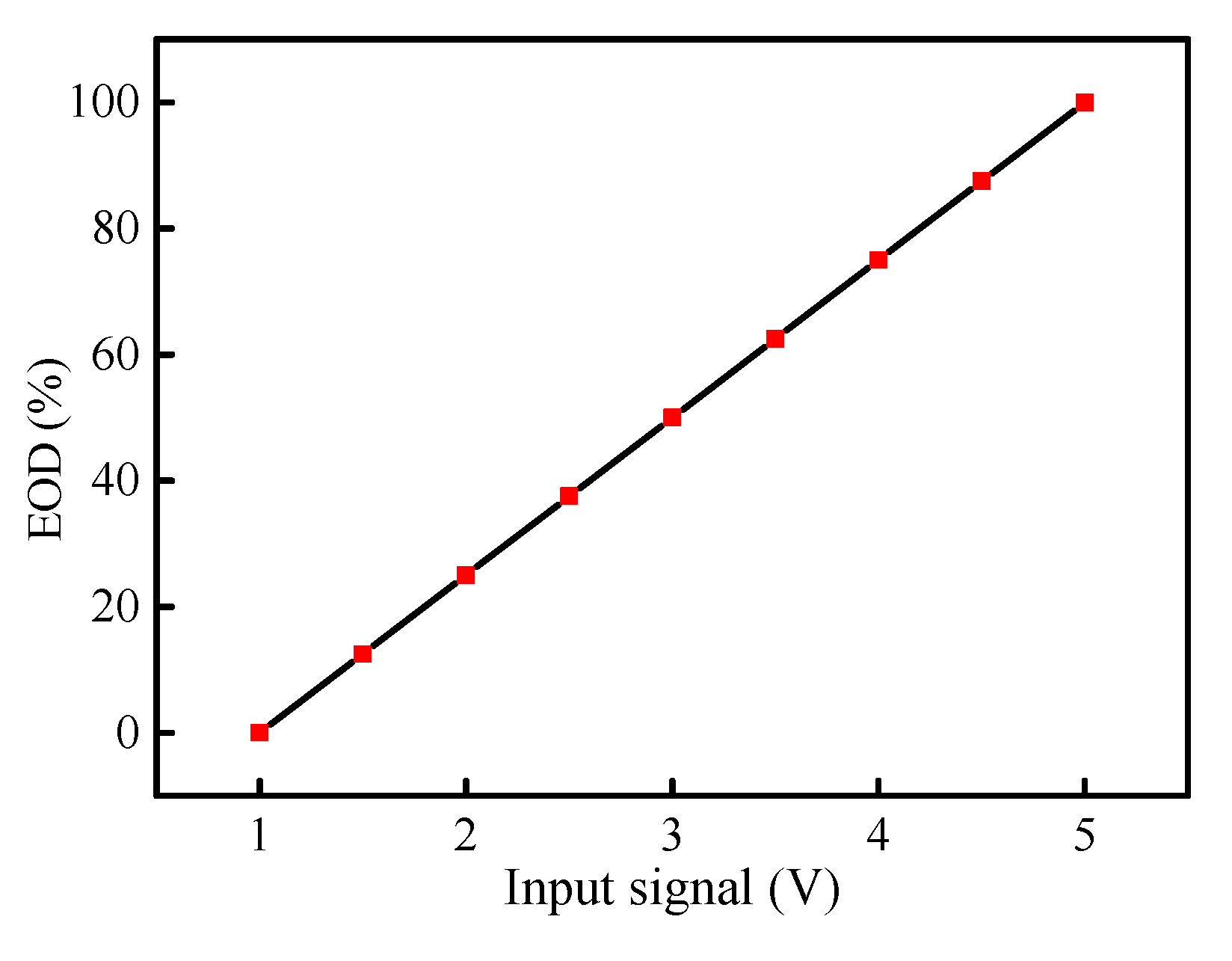
As shown in Figure 6, according to the relationship between the input signal of the stepping motor and EOD, a simulation model was established for the EX5-type expansion valve of Emerson. Its range of cooling capacity was from 4 kW to 39 kW for R134a refrigerant.

3.4. Compressor

Mass flow and energy change across the compressor is determined by experimentally identified volumetric and isentropic efficiencies (η_com,v and η_com,s). In the compressor, the fluid is assumed as a quasi-steady adiabat polytropic compression process. The displacement of compressor is constant, and its mass flow rate is calculated by the following formula:

$${\dot{m}}_{com\mathrm{s}}=ComS\cdot V_m\cdot {\rho }_R\cdot {\eta }_{com,v}$$

(23)

where ComS is the speed of compressor in rpm; ρ_R is the vapor density of compressor inlet in kg/m³; V_m is the volume in m²; and η_com,v is the volumetric efficiency of the compressor.

The compressor power can be calculated by the following formula:

$$T_{down}=T_{up}+\frac{T_{up}}{{\eta }_{is}}\left({\pi }^{1-1/\kappa }-1\right)$$

(24)

$$P_{com}=c_p\left(T_{down}-T_{up}\right)$$

(25)

where T_up is the upstream temperature in °C; T_down is the downstream temperature in °C; π is the pressure ratio; η_is is the adiabatic efficiency; and c_p is the specific heat in J/(kgK).

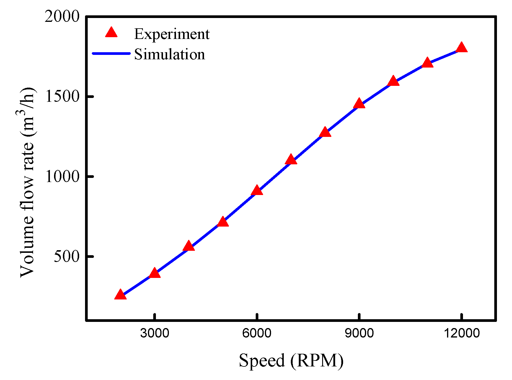
Based on the experimental data, the relationship between rotational speed and volume flow rate is fitted as follows:

$$V_{com}=-0.0238Com{S}^4-0.6447Com{S}^3+14.681Com{S}^2+98.447ComS+139.9$$

(26)

Figure 7 illustrates the relationship of the compressor speed and the corresponding volume flow rate.

4. Model Validation

4.1. Sensor Correction and Error Calculation

In this study, the temperature measurement accuracy of sensors was corrected before the experiment. The least square method was used to calibrate the sensors. Suppose that the ith pressure and jth temperature measured by the standard sensors are y_i and y_j, respectively, and the corresponding measured parameters are x_i and x_j. We transformed the measured values into the standard values through the following linear fitting formula:

$$\{\begin{array}{l}{y}_i=\tilde{a}{x}_i+\tilde{b}\\ y_j=\tilde{a}{x}_j+\tilde{b}\end{array}$$

(27)

By measuring a series of values at different pressures and temperatures, the values of $\tilde{a}$ and $\tilde{b}$ can be given as follows:

$$\{\begin{array}{l}\tilde{a}=\left({\displaystyle \sum _{i=1,j=1}^n{x}_{i,j}{y}_{i,j}-n\overline{x}\overline{y}}\right)/\left({\displaystyle \sum _{i=1,j=1}^n{x}_{i,j}{}^2-n{\overline{x}}^2}\right)\\ \tilde{b}=\overline{y}-\tilde{a}\overline{x}\end{array}$$

(28)

where $\overline{x}$ and $\overline{y}$ are the average values of x_i,j and y_i,j, respectively; n is the total number of measured data.

The average of all measurements in operation was used to estimate the temperature at each point in the test system. The accuracy limit of measurement was calculated as twice the standard deviation of experimental operation, and the population followed a symmetric unimodal normal distribution, within a 95% confidence interval [40,41]. The maximum calculated bias limit observed was ±0.38 °C during the thermistor calibration, which was negligible in the presence of the temperature measurements precision limit calculated during experimental system operation, which was assumed as the measurement uncertainty.

Inevitably, there are errors between simulation and experimental data, and they are calculated by Equation (29) as follows:

$$error=\frac{sd-ed}{ed}\cdot 100\%$$

(29)

where sd and ed represent the simulation and experimental data, respectively.

4.2. Evaporator Validation

An aluminum plate-fin evaporator was adopted in the helicopter TMS due to its compactness. The serrated fins of evaporator are shown in Figure 8a, and the structure of evaporator is shown in Figure 8b. The specific structural dimensions of the evaporator and its fins are shown in

Table 4. Structural parameters of condenser.

No.	Symbol	Parameter	Value (mm)
1	FinPeva	Fin pitch of evaporator	1
2	FinDeva	Fin depth of evaporator	1
3	FinTeva	Fin thickness of evaporator	0.1
4	FinHeva	Fin height of evaporator	1.5
5	FinOeva	Fin offset of evaporator	0.5
6	Leva	Length of evaporator	270
7	Heva	Height of evaporator	160
8	Weva	Width of evaporator	80

.

For the heat exchange areas of the refrigerant side used in the Equation (7) and the antifreeze side used in the Equation (16), they can be calculated, respectively, as follows:

$$A_{eva,R}\approx 2\cdot (Fin{P}_{eva}+Fin{H}_{eva})\cdot L_{eva}\cdot W_{eva}/Fin{P}_{eva}$$

(30)

$$A_{eva,A}\approx 2\cdot (Fin{P}_{eva}+Fin{H}_{eva})\cdot L_{eva}\cdot W_{eva}/Fin{P}_{eva}$$

(31)

where A_eva,R is the convective heat exchange area of the refrigerant side in m²; A_eva,A is the convective heat exchange area of antifreeze side in m²; FinP_eva is the fin pitch in m; FinH_eva is the fin height in m; L_eva is the length in m; and W_eva is the width in m.

Some experiments were performed to validate the plate-fin evaporator model. The experimental platform for the evaporator is shown in Figure 9a. The experimental prototype consisted of a refrigerant loop, an antifreeze loop, a data acquisition unit and a control unit. As seen Figure 9b, in the prototype, R134a flowing in the refrigerant loop is pumped into the water-cooled plate fin condenser (2) from the tested ARHEx (7). The subcooled refrigerant becomes the two-phase fluid after flowing through the dryer (1) and enters the EEV (3). Then it becomes slightly superheated vapor after passing through the ARHEx. In the antifreeze loop, an electric heater (10) works as the heat source. Antifreeze is pumped into the tested ARHEx (7), where it is cooled by cold refrigerant and then returns to the antifreeze tank (11). A mass flow meter (5) is equipped to measure the refrigerant mass flow rate in the refrigerant loop. The refrigerant side temperature and pressure used in this experiment were maintained by adjusting the compressor speed and the opening of EEV.

Resistance thermometers marked with T1 and T2 and pressure sensors marked with P1 and P2 were installed at the inlet of the EEV and the outlet of the ARHEx. The pressure difference between the inlet and outlet of ARHEx was obtained by a differential pressure transmitter marked with P0. Measurement of antifreeze flow rate was performed with a volume flow meter (8) with maximal relative measuring uncertainty of ±5%, and the antifreeze temperatures and pressure were measured with resistance thermometers marked with T3 and T4 and pressure sensors marked with P3 and P4 at the ARHEx inlet and outlet.

Table 5. Experimental conditions of evaporator.

No.	Symbol	Parameter	Value (mm)	Unit
1	Teva,out,R	Refrigerant outlet temperature	(19,21)	°C
2	Peva,out,R	Refrigerant outlet pressure	(520,540)	kPa
3	Teva,in,A	Antifreeze inlet temperature	(33,35)	°C
4	Peva,in,A	Antifreeze inlet pressure	(148,152)	kPa
5	qmeva,A	Antifreeze flow rate	3	m3/h
6	Teev,in,R	Inlet temperature of EEV	50	°C
7	Peev,in,R	Inlet pressure of EEV	1492	kPa

provides the detailed parameters for the experimental conditions, and the experimental data were processed to correct the simulation model.

In these experiments, a constant inlet enthalpy, a constant outlet temperature and a constant outlet pressure were kept for the cold side refrigerant; and a constant inlet temperature, a constant inlet pressure and a constant inlet volume flow were kept for the hot side antifreeze. The inlet mass flow rate of refrigerant was changed. After correcting the simulation model, the experimental and simulation results for the heat exchange capacity in the evaporator are shown in Figure 10. The error of heat exchange capacity between simulation result and experimental data was calculated by Equation (29).

Based on Figure 10, some conclusions can be observed when refrigerant flow rate varied from 350 to 700 kg/h:

• Figure 10a shows the comparison between experimental and simulation results for the heat exchange capacity when the refrigerant flow rate varies from 450–700 kg/h. The heat exchange capacity of the evaporator could reach 23.67 kW when the refrigerant flow rate reached 700 kg/h.
• Figure 10b shows the errors of heat exchange capacity between simulation results and experimental data, where the blue line and red line are boundary lines with error of 10%. The error range was within 0–10% under this condition. The results revealed that the error was the smallest when the refrigerant flow rate reached 600 kg/h. The evaporator model was validated in this way.

4.3. Condenser Validation

The parallel condenser consisted of 52 mini-channel tubes, as shown in Figure 11a, and had bulk dimensions of 640 mm × 370 mm × 20 mm. Four refrigerant flow channels were arranged in 24, 16, 7 and 6 channels, and each tube had 22 holes for uniform refrigerant distribution.

The material of the condenser used was aluminum, and the geometry of its louvered fin is shown in Figure 11a. Their main geometric parameters are described in

Table 6. Structural parameters of condenser.

No.	Symbol	Parameter	Value (mm)
1	FinPcon	Fin pitch of condenser	1.1
2	FinLcon	Fin length of condenser	5.4
3	FinTcon	Fin thickness of condenser	0.1
4	TubeHcon	External tube height of condenser	1.4
5	TubePcon	Tube periodicity of condenser	6.8
6	Lcon	Tube width of condenser	640
7	Hcon	Height of condenser	370

. The fin thickness was 0.1 mm, the louver pitch was 1 mm and the fin pitch was 1.1 mm. The louver angle was 30°. Each plate had 22 rectangular micro-channels, and each size was 0.65 mm × 0.9 mm.

For the heat exchange area of air side used in the Equation (21), it can be calculated as follows:

$$\begin{array}{ll}{A}_{con,a}& \approx 4\cdot A_{cross}\cdot L_{tube}/D_{con,a}\\ & =4\cdot A_a\cdot {L_{tube}}^2/(D_{con,a}\cdot Fin{P}_{con})\end{array}$$

(32)

where A_con,a is the convective heat exchange area in m²; A_cross is the air side cross section area in m²; L_tube is the length of tube in m; D_con,a is the air side fin hydraulic diameter in mm; A_a is the air side cross sectional area per fin and per tube in m²; FinP_con is the fin pitch in m. The heat exchange area of the air side was 8.017454 m².

Experiments were conducted to validate the condenser simulation model. The experimental platform for the condenser is shown in Figure 12.

The constant temperature and humidity in the environment simulation chamber are control by a temperature humidity control (THC) unit. The constant temperature and pressure for the R134a used in this experiment were controlled by a small vapor refrigeration cycle (SVRC). A small cabin was put in the environment simulation chamber, and its cabin temperature was controlled by the tested condenser. The temperatures of the air side inlet and outlet were measured by sensors, respectively. The refrigerant side temperature and pressure were maintained by adjusting the compressor speed and the expansion valve in the SVRC. The refrigerant mass flow rate was recorded by a mass flow meter.

Table 7. Experimental conditions of condenser.

No.	Symbol	Parameter	Value	Unit
1	Tcon,in,a	Air inlet temperature	(38.5,41.5)	°C
2	Vcon,in,a	Air inlet velocity	1,2,3,4,5,6	m/s
3	Pcon,in,a	Air inlet pressure	(99,101)	kPa
4	Rhcon,in,a	Relative humidity	(35,45)	%
5	SC	Sub-cooling	(−9,−7)	°C
6	Tcon,in,R	Refrigerant inlet temperature	(98.5,101.5)	°C
7	Pcon,in,R	Refrigerant inlet pressure	(1.5,1.54)	kPa

provides the detailed specifications for the test condition, and the experimental data were processed to correct the simulation model.

In these experiments, a constant air inlet temperature, a constant air inlet pressure and a constant air inlet relative humidity were kept for the cold side air; and a constant inlet temperature, a constant inlet pressure and a constant outlet sub-cooling were kept for the hot side antifreeze. The air inlet velocity was changed.

After correcting the simulation model, the experimental and simulation results for the temperature and pressure in the condenser are shown in Figure 13. Based on Figure 13, some observations could be made when the air flow rate varied from 1 m/s to 6 m/s:

• Figure 13a,b show the outlet temperatures of the refrigerant side and air side. With the increase of the air speed, the outlet temperature of refrigerant side, T_con,out,R, and the outlet temperature of air side, T_con,out,a, in the condenser decreased accordingly. When the air speed reached 6 m/s, the T_con,out,R and T_con,out,a reached 44 °C and 50 °C, respectively.
• Figure 13c,d show the outlet pressures of the refrigerant side and air side in the condenser. Regarding the parallel condenser, with the increase of the air speed of the condenser fan, the outlet pressure of the refrigerant side, △P_con,R, and the outlet pressure of the air side, △P_con,a, in the condenser increased accordingly. When the fan air speed reached 6 m/s, the △P_con,R reached 107 kPa and the △P_con,a reached 192 Pa.
• The errors of T_con,out,R, T_con,out,a, △P_con,a and △P_con,R between simulation results and experimental data were calculated by Equation (29). After the models were calibrated, the errors were less than 5%. The condenser simulation model had relatively stable reliability and could be applied in the simulation study.

5. System Control Performance Analysis

5.1. System Simulation Condition

Two extreme simulation conditions were studied to investigate the performance of the control strategy. They were a cold day condition and a hot day condition. The corresponding ambient temperatures in the conditions were −40 °C and 40 °C, respectively. For clarity, the parameters of simulation cases used in this study are presented in

Table 8. Parameters of simulation cases.

No.	Parameter	Cold Day Condition	Hot Day Condition	Unit
1	Ambient air temperature on ground	−40	40	°C
2	Ambient air density	(0.6,1.25)	(0.6,1.25)	kg/m3
3	Ambient air pressure	(0.4,1)	(0.4,1)	bar
4	Ambient air relative humidity	(5,40)	(5,40)	%
5	Air speed of fan	1	5	m/s
6	Avionics heat load	(10,15)	(10,15)	kW

.

In order to test the performance of the control strategy, the same given flight envelope was used to reflect two conditions, as shown in Figure 14a. Similarly, the air density was the same under both conditions, as seen in Figure 14b. Figure 14c shows the ambient air temperature; the ground temperature of the cold day condition was chosen as its extreme point, −40 °C, and the temperature change of ram air was from −40 °C to −50 °C. Meanwhile, the ground temperature of the hot day condition was chosen as its extreme point, 40 °C. As listed in Table 8, the air speed of the condenser fan was 1 m/s for the cold day condition and 5 m/s for the hot day condition. Figure 14d shows the heat load of avionics. It had seven continuous step stages, namely 12 kW, 15 kW, 14 kW, 15 kW, 13 kW, 14 kW and 13.5 kW. However, there was a preheating process in the cold day condition. After 136 s of the preheating process, the antifreeze temperature reached 5 °C in the cold simulation condition, and its heating device was closed. The helicopter TMS was controlled according to the control strategy mentioned in Section 2.2.

5.2. Control Performance in the Cold Day Condition

5.2.1. Control Target Performance

The control target value of SH was set at 5 °C, which was a compromise between the working performance and the minimum steady superheat. The desired operating temperature is 20 °C for avionics. With the control strategy, the changes of ComS, EOD, temperature and COP are shown in Figure 15.

Based on Figure 15, some conclusions can be observed:

• Figure 15a,b show the control results of ComS and EOD, respectively. The valves of ComS and EOD were 0 at 0–136 s, that is, the compressor and the EEV did not begin working. The reason is that the antifreeze in the ALC loop was lower than 5 °C and it should have been preheated, and the VCR loop did not start at all. After the preheating process, the VCR began to start up. In the initial startup stage, the thermal characteristics of the refrigerants were not uniform in the pipeline. After a period of time, the thermal characteristics of the refrigerants became stable. Correspondingly, ComS and EOD reached their stable values, namely 1800 rev/min and 35%, from 136 to 200 s, respectively. The change of heat load led to the corresponding seven step changes of ComS and EOD. The corresponding values of ComS were 1825 rev/min, 2375 rev/min, 2200 rev/min, 2375 rev/min, 2000 rev/min, 2150 rev/min and 2125 rev/min. The corresponding values of EOD were 35.5%, 42.5%, 39.4%, 42.6%, 36.8%, 40.1% and 38.7%. The trends of the control curve for ComS and EOD were similar to the heat load curve, and their response times lagged slightly behind the heat load curve.
• Figure 15c shows the control response of temperatures at the inlet and outlet of the cold plate when the helicopter completed a given flight envelope in 12,000 s. T_cp,in could be controlled at 20 °C. T_cp,out varied with the heat load of the avionics. The control error bands of T_cp,in were both within ±1 °C. There were seven small fluctuations in the control curve of T_cp,out, which were caused by the heat load change.
• The control performance of SH is illustrated in Figure 15d. SH could be maintained around 5 °C regardless of the changes in the heat load and the working environment. There were also seven fluctuations in the curve of SH. SH is related to the mass flow rate of refrigerant. The change of heat load led to the change of heat transferred from the ALC loop to the VCR loop. Then ComS and EOD were correspondingly changed in order to control the target temperature, which conversely led to the change of mass flow rate of VCR.
• COP of the VCR loop is illustrated in Figure 15e, and it could be maintained around 6 after the system was stable. The change trends of COP and heat load were very similar.
• Figure 15f shows the control response of SC, which could be maintained at −4.5 °C. To maintain the system stable and reliable, SH and SC must be controlled as stable as possible.

5.2.2. p-h Performance

Figure 16 describes the pressure-enthalpy (p-h)diagrams of the VCR loop under the cold day condition when the flight altitude widely varied from 0 to 6000 m in 12,000 s.

From Figure 16, we can observe some conclusions as follows:

• Figure 16 describes the p-h diagram of the VCR loop when the flight altitude was 750 m and the flight time was 1500 s. At this time, the heat load was 12 kW, the evaporation temperature was 11 °C, and the condensation temperature was 40 °C. SH was 5 °C, SC was −4.5 °C, and COP was maintained at about 6.
• Figure 16 shows the p-h diagrams of the VCR loop when the flight altitudes were 3 km, 1.5 km and 0 m, respectively. The corresponding heat loads were 15 kW, 14 kW and 13.5 kW. The corresponding evaporation temperatures were 11 °C, 9 °C and 15 °C. The corresponding condensation temperatures were 41 °C, 38 °C and 45 °C.
• In the whole given flight envelope, the p-h diagrams of the VCR loop did not change significantly. The evaporation and condensation temperatures usually effect the change of the p-h diagram. The ram air temperature was in the range of −50 °C to −45 °C, which made the condenser work with good performance. Both temperatures of evaporation and condensation were relatively low and stable, so that the change of the p-h diagram was not obvious in the cold day condition.

5.3. Control Performance in the Hot Day Condition

5.3.1. Control Target Performance

The control target values of SH and T_cp,in remained 5 °C and 20 °C, separately, for the reasons stated previously. With the control strategy, the changes of ComS, EOD, temperature and COP are shown in Figure 17.

As seen in Figure 17, we could observe that the control strategy could effectively remove the heat load of high-power avionics. Some conclusions can be observed:

• ComS and EOD could be maintained around their controlled set points. Figure 17a shows the control results of ComS and EOD over time, respectively. The heat load curve of avionics had seven step stages, and it led to the corresponding changes of ComS and EOD. When the heat load changed from 12 kW to 15 kW, ComS was controlled from 3500 rev/min to 4263 rev/min. The corresponding value of EOD was from 50% to 68%. The curve trend of ComS and EOD was similar to the heat load curve of avionics. However, the values of ComS and EOD in seven stages were on average higher than those under the cold day condition. The temperature of ram air under the hot day condition was higher, and the change range from 3 °C to 40 °C was larger than that under the cold day condition. In order to meet the control requirement, it needed to transfer more heat load into the ram air, which led to the increase of compressor power consumption. Therefore, ComS and the adjusted range of EOD were larger than those in the cold day condition.
• The control performance of temperature at the inlet and outlet of the cold plate and SH are illustrated in Figure 17b. T_cp,in could be controlled at 20 °C and its control error band was within ±1 °C. T_cp,out could be controlled within the range from 22 °C to 24 °C. There were also seven small fluctuations in the control curve of T_cp,out, which were caused by the heat load. SH could be maintained around 5 °C regardless of the changes of the heat load and flight environment.
• The COP of the VCR loop is illustrated in Figure 17c. The COP could be maintained in the range of 2.58–4.9. The environment condition was the worst when the helicopter was in the ground standby state. This led to more power consumption of the compressor. Compared with the control curve in the cold day condition, the sudden change time point of COP was not consistent with that of the heat load of avionics under the hot day condition. The reason was that COP is related to the temperature of ram air. The higher-temperature ram air led to the increase of power consumption of the compressor accordingly. This made COP different from that in the cold day condition.
• Figure 17d shows the control response of SC; it could be maintained at −5 °C, which was lower than that of the cold day condition.

5.3.2. p-h Performance

Figure 18 describes the p-h diagrams of VCR loop under the hot day condition when the flight altitude varied from 0 to 6000m within 12,000 s.

Some conclusions can be obtained from Figure 18 as follows:

• Figure 18 shows the p-h diagram of the VCR loop when the flight altitude was 750 m and flight time was 1500 s. At this time, the heat load was 12 kW, SH was 5 °C, SC was −5 °C, and COP was 2.68. The evaporation and condensation temperatures were 15 °C and 75 °C, respectively. The corresponding evaporation and condensation pressures were 4.88 bar and 23.14 bar. The outlet enthalpy values of evaporator and condenser were 411.69 kJ/kg and 300.75 kJ/kg, respectively.
• Figure 18 shows the p-h diagrams of the VCR loop when the flight altitudes were 3 km, 1.5 km and 0 m. The corresponding heat loads were 15 kW, 14 kW and 13.5 kW. The ram air temperature varied greatly from 3 °C to 40 °C. The condensation temperatures varied noticeably at different heat load points. They were 65 °C, 69 °C and 76 °C at 3000 s, 9000 s and 12,000 s, respectively. The evaporation temperatures were 11 °C, 9 °C and 15 °C, respectively. COP changed from 2.58 at 0 m to 4.9 at 6000 m.
• Compared with the p-h diagrams of the VCR loop in the cold day condition, as seen in Figure 16, the p-h diagrams in Figure 18 changed greatly in the hot day condition. The values of condensation temperature or condensation pressure in the hot day condition were normally larger than the ones in the cold day condition. This change was caused by the following reasons: The ram air temperature changed noticeably from 40 °C at 0 m to 3 °C at 6000 m, which made the condenser temperature change in a large range. In addition, a higher speed of the condenser fan, namely 5 m/s, was used in the hot day condition.

5.4. Robustness Analysis

For the VCR system, the control models of thermodynamic control volumes were established in the refrigerant side by using the methods mentioned in the literature [35]. Hence, the control models developed are reliable. The variation of uncontrolled parameters is one of the important factors that affect the system performance. These are part of the system model and may strongly affect the behavior of the system. Robustness is a characteristic of that controller which minimizes the effect of uncertainty or variation in system parameters without eliminating the source of the uncertainty or variation.

Air temperature may be the most important uncontrollable parameter that affects system behavior. To show the controller robustness, we assumed that the outside air temperature, an uncontrolled parameter, varied according to the hot day condition during the simulation, while other conditions and parameters remained unchanged. As can be seen from Figure 19, the controller response during temperature changes was quite reasonable, and this controller was also robust to temperature variation.

6. Conclusions

A helicopter TMS based on and ALC loop and VCR loop is proposed in order to meet the cooling requirements of high-power avionics working in extremely conditions. Its control strategy is further studied in order to maintain the control performance in different flight conditions. Some experiments are conducted to validate the models of evaporator and condenser in the helicopter TMS. Then, the simulation work of the helicopter TMS is carried out to evaluate the performance of the control strategy. Two extreme weather conditions, the cold day condition and the hot day condition, are used to test the control performance. The simulation results show that the proposed control strategy can ensure the stability of the helicopter TMS in extreme weather conditions. The main conclusions are summarized as follows:

• Under the cold day condition, the ram air temperature is from −40 °C to −50 °C. It is necessary to preheat the antifreeze in the liquid cooling system, which can effectively reduce the flow resistance and the power consumption of the pump. When the heat load changes from 12 kW to 15 kW, the variation ranges of ComS and EOD are 1825–2375 rev/min and 35.5–42.6%, respectively. SH and SC can be controlled very well. T_cp,out varies with the heat load but it can remain about 23 °C, and the control error band of T_cp,in is within ±1 °C. COP is around 6 in the steady state. In the whole given flight envelope, the p-h diagrams of the VCR loop do not change significantly due to the temperatures of evaporation and condensation being relatively low and stable.
• Under the hot day condition, the ram air temperature is from 3 °C to 40 °C. When the heat load changes from 12 kW to 15 kW, the variation ranges of ComS and EOD are 3500 to 4263 rev/min and 50–68%, respectively. SH and SC can be controlled very well. T_cp,out varies from 22 °C to 24 °C, and the control error band of T_cp,in is within ±1 °C. The range of COP is from 2.58 at 0 m to 4.9 at 6000 m, and it is lower than that in the cold day condition. In the whole given flight envelope, the p-h diagrams of the VCR loop change greatly due to the obvious change of ram air temperature and a higher speed of the condenser fan.

References

1. Sarafraz, M.M.; Arjomandi, M. Thermal performance analysis of a microchannel heat sink cooling with copper oxide-indium (CuO/In) nano-suspensions at high-temperatures. Appl. Therm. Eng. 2018, 137, 700–709. [Google Scholar] [CrossRef]
2. Dadsetani, R.; Sheikhzadeh, G.A.; Hajmohammadi, M.R.; Safaei, M.R. Introduce a novel configuration of microchannel and high-conductivity inserts for cooling of disc-shaped electronic components. Int. J. Heat Fluid Flow 2019. [Google Scholar] [CrossRef]
3. Sarafraz, M.; Hormozi, F.; Nikkhah, V. Thermal performance of a counter-current double pipe heat exchanger working with COOH-CNT/water nanofluids. Exp. Therm. Fluid Sci. 2016, 78, 41–49. [Google Scholar] [CrossRef]
4. Salari, E.; Peyghambarzadeh, S.; Sarafraz, M.; Hormozi, F.; Nikkhah, V. Thermal behavior of aqueous iron oxide nano-fluid as a coolant on a flat disc heater under the pool boiling condition. Heat Mass Transf. 2017, 53, 265–275. [Google Scholar] [CrossRef]
5. Ma, K.; Liu, J. Liquid metal cooling in thermal management of computer chips. Front. Energy Power Eng. Chin. 2007, 1, 384–402. [Google Scholar] [CrossRef]
6. Sarafraz, M.; Hormozi, F. Convective boiling and particulate fouling of stabilized CuO-ethylene glycol nanofluids inside the annular heat exchanger. Int. Commun. Heat Mass Transf. 2014, 53, 116–123. [Google Scholar] [CrossRef]
7. Deymi-Dashtebayaz, M.; Maddah, S.; Goodarzi, M.; Maddah, O. Investigation of the effect of using various HFC refrigerants in geothermal heat pump with residential heating applications. J. Therm. Anal. Calorim. 2020. [Google Scholar] [CrossRef]
8. Michalak, T.; Emo, S.; Ervin, J. Control strategy for aircraft vapor compression system operation. Int. J. Refrig. 2014, 48, 10–18. [Google Scholar] [CrossRef]
9. Emo, S.; Ervin, J.; Michalak, T.E.; Tsao, V. Cycle-Based Vapor Cycle System Control and Active Charge Management for Dynamic Airborne Applications; SAE Technical Paper; SAE International: Warrendale, PA, USA, 2014. [Google Scholar]
10. Chen, Y.; Deng, S.; Xu, X.; Chan, M. A study on the operational stability of a refrigeration system having a variable speed compressor. Int. J. Refrig. 2008, 31, 1368–1374. [Google Scholar] [CrossRef]
11. Otten, R.J. Superheat Control for Air Conditioning and Refrigeration Systems: Simulation and Experiments; Illinois Digital Environment for Access to Learning and Scholarship: Champaign, IL, USA, 2010. [Google Scholar]
12. Jain, N.; Alleyne, A. Exergy-based optimal control of a vapor compression system. Energy Convers. Manag. 2015, 92, 353–365. [Google Scholar] [CrossRef] [Green Version]
13. De Oliveira, V.; Trofino, A.; Hermes, C.J.L. A switching control strategy for vapor compression refrigeration systems. Appl. Therm. Eng. 2011, 31, 3914–3921. [Google Scholar] [CrossRef]
14. Yan, G.; Liu, Y.; Qian, S.; Yu, J. Theoretical study on a vapor compression refrigeration system with cold storage for freezer applications. Appl. Therm. Eng. 2019, 160, 114091. [Google Scholar] [CrossRef]
15. Liang, K.; Li, Z.; Chen, M. Comparisons between heat pipe, thermoelectric system, and vapour compression refrigeration system for electronics cooling. Appl. Therm. Eng. 2019, 149, 260–267. [Google Scholar] [CrossRef]
16. Chen, M.; Snyder, J. Analytical and numerical parameter extraction for compact modeling of thermoelectric coolers. Int. J. Heat Mass Transf. 2013, 60, 689–699. [Google Scholar] [CrossRef]
17. Zhao, L.; Cai, W.; Ding, X.; Chang, W. Decentralized optimization for vapor compression refrigeration cycle. Appl. Therm. Eng. 2013, 51, 753–763. [Google Scholar] [CrossRef]
18. Marcinichen, J.B.; Holanda, T.N.; Melo, C. A dual siso controller for a vapor compression refrigeration system. In Proceedings of the International Refrigeration and Air-Conditioning Conference, West Lafayette, IN, USA, 14–17 July 2008. [Google Scholar]
19. Rasmussen, B.P.; Alleyne, A.G. Control-oriented modeling of transcritical vapor compression systems. J. Dyn. Syst. Measur. Control 2004, 126, 54–64. [Google Scholar] [CrossRef]
20. Rasmussen, B.P.; Alleyne, A.G. Dynamic Modeling and Advanced Control of Air Conditioning and Refrigeration Systems; Air Conditioning and Refrigeration Center, College of Engineering University of Illinois at Urbana-Champaign: Champaign, IL, USA, 2006. [Google Scholar]
21. Elliott, M.S.; Rasmussen, B.P. On reducing evaporator superheat nonlinearity with control architecture. Int. J. Refrig. 2010, 33, 607–614. [Google Scholar] [CrossRef]
22. Li, H.; Jeong, S.-K.; You, S.-S. An empirical model for independent control of variable speed refrigeration system. Appl. Therm. Eng. 2008, 28, 1918–1924. [Google Scholar] [CrossRef]
23. Anurag, G.; Marcel, A.S.; Srinivas, G. A review of control methodologies for vapor compression and absorption heat pumps. Int. J. Refrig. 2019, 97, 1–20. [Google Scholar]
24. Zhihui, W.; Du, R. Design and experimental study of a miniature vapor compression refrigeration system for electronics cooling. Appl. Therm. Eng. 2011, 31, 385–390. [Google Scholar]
25. Jain, N.; Alleyne, A.G. Thermodynamics-based optimization and control of vapor-compression cycle operation: Optimization criteria. In Proceedings of the American Control Conference (ACC), San Francisco, CA, USA, 29 June–1 July 2011; pp. 1352–1357. [Google Scholar]
26. Li, H.; Jeong, S.-K.; You, S.-S. Feedforward control of capacity and superheat for a variable speed refrigeration system. Appl. Therm. Eng. 2009, 29, 1067–1074. [Google Scholar] [CrossRef]
27. Tian, J.; Feng, Q.; Zhu, R. Analysis and experimental study of MIMO control in refrigeration system. Energy Convers. Manag. 2008, 49, 933–939. [Google Scholar] [CrossRef]
28. Yang, Z.; Pollock, D.T.; Wen, J.T. Optimization and predictive control of a vapor compression cycle under transient pulse heat load. Int. J. Refrig. 2017, 75, 14–25. [Google Scholar] [CrossRef] [Green Version]
29. Xu, Y.; Zhang, S.; Xiao, Y. Modeling the dynamic simulation and control of a single effect Libr–H2o absorption chiller. Appl. Therm. Eng. 2016, 107, 1183–1191. [Google Scholar] [CrossRef]
30. Grauso, S.; Mastrullo, R.; Mauro, A.W.; Thome, J.R.; Vanoli, G.P. Flow pattern map, heat transfer and pressure drops during evaporation of R-1234ze(E) and R134a in a horizontal, circular smooth tube: Experiments and assessment of predictive methods. Int. J. Refrig. 2013, 36, 478–491. [Google Scholar] [CrossRef]
31. Tao, W.; Hongbo, Z.; Dalin, Z.; Lin, L. Development of evaporation pressure-capacity control strategy for aircraft vapor cycle system. Int. J. Refrig. 2017, 83, 14–22. [Google Scholar]
32. Aprea, C.; Renno, C. Experimental analysis of a transfer function for an air cooled evaporator. Appl. Therm. Eng. 2001, 21, 481–493. [Google Scholar] [CrossRef]
33. Wang, T.; Gu, B.; Wu, B.; Ma, H.; Qian, C. Modeling for multi-pass parallel flow condenser with the effect of refrigerant mal-distribution. Int. J. Refrig. 2015, 60, 234–246. [Google Scholar] [CrossRef]
34. Tuo, H.; Hrnjak, P. Effect of the header pressure drop induced flow maldistribution on the microchannel evaporatorperformance. Int. J. Refrig. 2013, 36, 2176–2186. [Google Scholar] [CrossRef]
35. Min, G.R. Thermal Control Technology of Satellite; China Astronautic Publishing House: Beijing, China, 1991. (In Chinese) [Google Scholar]
36. Park, I.; Lee, H.; Mudawar, I. Determination of flow regimes and heat transfer coefficient for condensation in horizontal tubes. Int. J. Heat Mass Transf. 2015, 80, 698–716. [Google Scholar] [CrossRef]
37. Zajaczkowski, B.; Halon, T.; Krolicki, Z. Experimental verification of heat transfer coefficient for nucleate boiling at sub-atmospheric pressure and small heat fluxes. Heat Mass Transf. 2016, 52, 205–215. [Google Scholar] [CrossRef]
38. Gianluigi, A.M.; Benini, E. Performance of a turboshaft engine for helicopter applications operating at variable shaft speed. In Proceedings of the ASME 2012 Gas Turbine India Conference, Mumbai, Maharashtra, India, 1 December 2012. [Google Scholar]
39. Xianglong, L.; Zhitong, Y.; Ziwei, C.; Ying, C.; Songping, M. Performance comparison of the liquid–vapor separation, parallel flow, and serpentine condensers in the organic Rankine cycle. Appl. Therm. Eng. 2016, 94, 435–448. [Google Scholar]
40. Kim, J.H.; Simon, T.W.; Viskanta, R. Journal of heat transfer policy on reporting uncertainties in experimental measurements and results. ASME J. Heat Transf. 1993, 115, 5–6. [Google Scholar] [CrossRef] [Green Version]
41. Nunes, T.K.; Vargas, J.V.C.; Ordonez, J.C. Modeling, simulation and optimization of a vapor compression refrigeration system dynamic and steady state response. Appl. Energy 2015, 158, 540–555. [Google Scholar] [CrossRef]
Figure 1. Schematic diagram of thermal management system (TMS) based on antifreeze liquid cooling (ALC) and vapor compression refrigeration (VCR) loops (E1, EEV; E2, condenser; E3, fan; E4, mass flow meter; E5, compressor; E6, electric motor; E7, cold plate; E8, evaporator; E9, temperature control valve; E10, relief valve; E11, heater; E12, antifreeze tank; E13, pump; E14, volume flow meter; T0, ground ambient temperature; T, temperature sensor; P, pressure sensor).
Energies 13 02177 g001
Figure 2. Coupled control strategy of SH and Tcp,in.
Energies 13 02177 g002
Figure 3. Feedforward control.
Energies 13 02177 g003
Figure 4. Relationship of pump power consumption and physical parameters.
Energies 13 02177 g004
Figure 5. Control strategy of TMS.
Energies 13 02177 g005
Figure 6. Relationship of input signal and opening.
Energies 13 02177 g006
Figure 7. Volume flow rates of compressor in simulation and experiment.
Energies 13 02177 g007
Figure 8. Schematic diagram of evaporator.
Energies 13 02177 g008
Figure 9. Experimental platform and its schematic of the experimental facility.
Energies 13 02177 g009
Figure 10. Simulation and experimental data comparison of evaporator.
Energies 13 02177 g010
Figure 11. Structure of condenser.
Energies 13 02177 g011
Figure 12. Experimental platform and its measurement points.
Energies 13 02177 g012
Figure 13. Pressure and temperature comparison in the condenser.
Energies 13 02177 g013
Figure 14. Simulation conditions.
Energies 13 02177 g014
Figure 15. Control results in a cold day.
Energies 13 02177 g015
Figure 16. p-h diagrams of VCR in thermal management in a cold day.
Energies 13 02177 g016
Figure 17. Control results in a hot day.
Energies 13 02177 g017
Figure 18. p-h diagrams of VCR in thermal management in a hot day.
Energies 13 02177 g018
Figure 19. Antifreeze inlet temperature of cold plate during temperature variation.
Energies 13 02177 g019