Self-Attention Network for Partial-Discharge Diagnosis in Gas-Insulated Switchgear

Abstract

Detecting, measuring, and classifying partial discharges (PDs) are important tasks for assessing the condition of insulation systems used in different electrical equipment. Owing to the implementation of the phase-resolved PD (PRPD) as a sequence input, an existing method that processes sequential data, e.g., the recurrent neural network, using a long short-term memory (LSTM) has been applied for fault classification. However, the model performance is not further improved because of the lack of supporting parallel computation and the inability to recognize the relevance of all inputs. To overcome these two drawbacks, we propose a novel deep-learning model in this study based on a self-attention mechanism to classify the PD patterns in a gas-insulated switchgear (GIS). The proposed model uses a self-attention block that offers the advantages of simultaneous computation and selective focusing on parts of the PRPD signals and a classification block to finally classify faults in the GIS. Moreover, the combination of LSTM and self-attention is considered for comparison purposes. The experimental results show that the proposed method achieves performance superiority compared with the previous neural networks, whereas the model complexity is significantly reduced.

1. Introduction

The popularity of power systems is rapidly increasing as the power demand increases, and the reliability of a power grid is important for a stable power-system operation. Gas-insulated switchgears (GISs) are equipment filled with ${\mathrm{SF}}_6$ gas that have excellent insulation characteristics and have been applied to substation equipment as the main protection device since the late 1960s owing to their high reliability, safety, and compactness [1]. Various failures can occur with the passage of service time, and the insulation defects in a GIS can cause partial discharges (PDs) before breakdown [2,3,4]. Therefore, detecting PDs at the early stages contributes to ensuring high reliability and safety of grid assets [5].

The PDs in a GIS can be measured using electrical, mechanical, and chemical methods [6,7]. High-frequency and ultra-high-frequency (UHF) sensors are used in the electrical methods [4,8,9], acoustic sensors are used for sound measurements [10,11], and dissolved-gas analysis is employed in the chemical methods [12,13]. In particular, the UHF method offers the advantage of high-sensitivity detection [14]. Therefore, the UHF measurement-system verification method has been standardized [15]. The present study uses a UHF sensor for a PD measurement system.

To examine the characteristic of PDs in a GIS, two types of analyses that have been studied are available, namely, time-resolved PD (TRPD) and phase-resolved PD (PRPD) [16,17,18,19,20,21,22,23]. In the TRPD method, the time-domain, frequency-domain, and both time- and frequency-domain features are used to analyze the PD pulses [21,22,23]. The PRPD-based method analyzes the phase–amplitude–number $(\varphi -q-n)$ measurements, where $\varphi$ is the phase angle, q is the amplitude, and n is the phase angle, q is the amplitude, and n is the number of discharges [24]. The number of PD pulses, maximum amplitude, or average amplitude in each phase is used as features in the PD classification [25].

Most of the previous studies on PD analysis using PRPDs focused on either extracting the useful features or accurate classification based on these extracted features. Signal-processing techniques such as time-domain [26], frequency-domain [27], and time–frequency-domain [28] analyses are used to extract the representative features from PRPDs. After feature extraction, the dimension reduction for computational efficiency is achieved through a feature-selection step. Correlation analysis is applied to cluster the PDs into different groups [29]. Principal component analysis is used to reduce the dimensions [30,31]. Based on the useful features from the univariate phase-resolved distributions [32], the final step is to train the classifiers such as neural networks [33], decision trees [34], and support vector machines (SVMs) [35]. However, the PD classification performance significantly varies depending on the particular combination of the existing feature-extraction and classification methods. Therefore, to maximize the PD classification performance, an integrated framework simultaneously considering both the feature-extraction and classification methods is needed.

Motivated by this objective, a deep-learning model is proposed to combine the automatic feature-extraction and fault-classification methods [36,37] in which deep neural networks (DNNs) have recently achieved cutting-edge performance in pattern-recognition tasks such as computer vision, speech recognition, text classification, and many other domains [38,39,40]. More recently, deep-learning methods have been applied to PRPD classification. DNNs [41] and convolutional neural networks (CNNs) [42] are proposed to improve the recognition accuracy of PRPDs. CNNs allow the systems to learn the local response from temporal or spatial data; however, they lack the ability to learn the sequential correlations of the inputs. Recurrent neural networks (RNNs) with a long short-term memory (LSTM) have advantages over the CNN because the models can effectively process the sequential data [43]. However, the sequential characteristic of RNN-based models does not assist parallelism, which results in the significant training processing time when the input sequence is long [44].

To overcome the aforementioned drawbacks, we propose new classification methods to classify faults in a GIS using PRPDs, namely, self-attention-based neural network for PRPDs (SANPD) and LSTM SANPD (LSANPD) methods. Self-attention takes advantage of parallel computation and enables the capture of the interactions among inputs [45] because the self-attention function can capture the global dependence of the entire input without requiring recurrence or convolution components [44]. In LSANPD, the combination of LSTM and the self-attention mechanism further improves the performance, because the self-attention mechanism can address the lack of simultaneous computation and focus on the important information from the LSTM inputs.

The proposed SANPD and LSANPD methods employ multi-head self-attention, feed-forward networks, and a classification layer. The multi-head self-attention is used to jointly attend to the information from different representation subspaces that correspond to the different phase sets of PRPDs. The feed-forward networks overcome the lack of self-attention, which is a linear model, because of the composite mapping of the nonlinear processing units [44]. Finally, the classification layer is employed to detect faults in the GIS. The main contributions of this paper are summarized as follows:

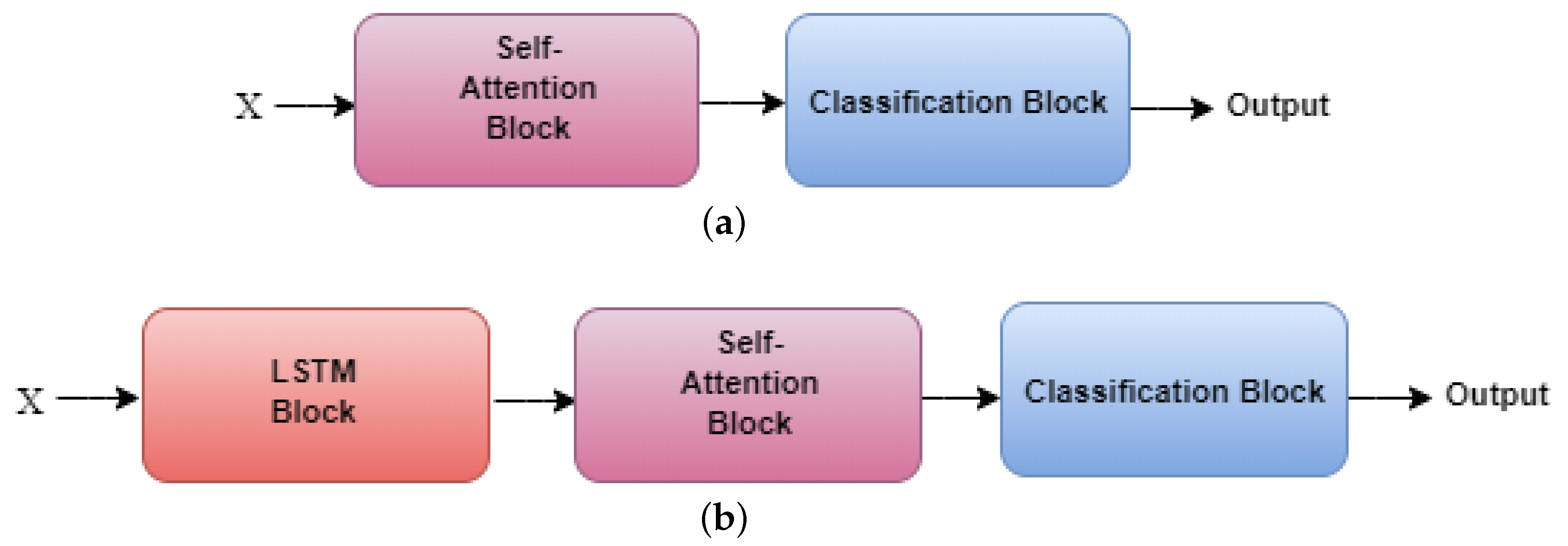
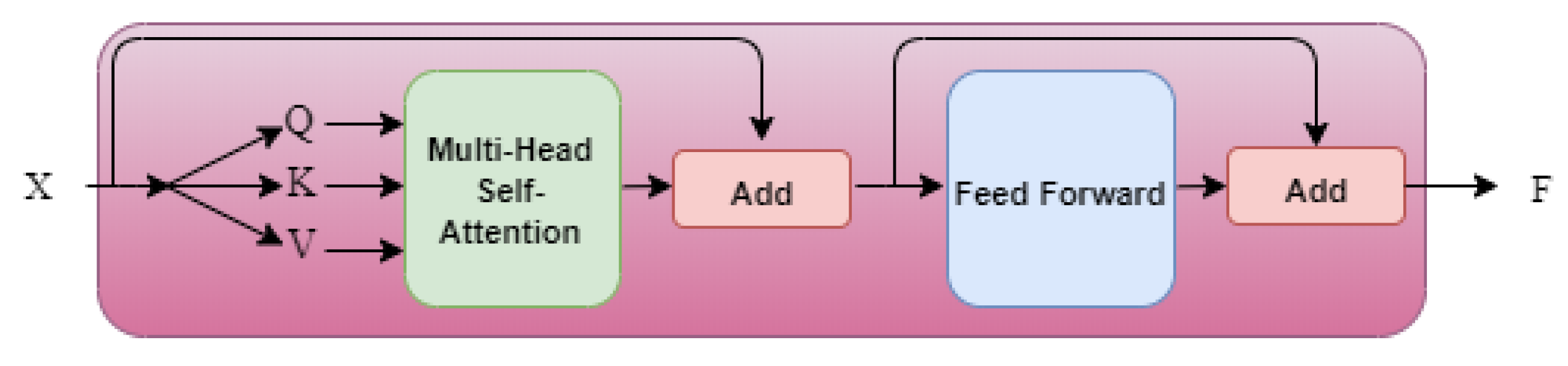
• Self-attention is introduced for the first time to classify the PRPDs in a GIS. Self-attention offers the advantages of classification accuracy and computational efficiency compared with DNNs, CNNs, and RNNs [41,42,46] because it can capture the relevance among the phases of the PRPDs by considering their entire interaction sequence input regardless of distance [44].
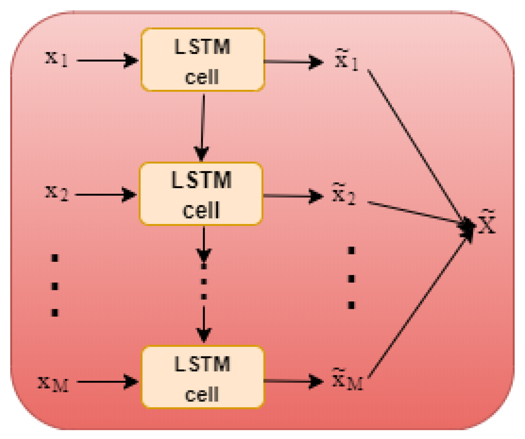
• The LSTM self-attention method is also considered. In the LSTM self-attention model, the self-attention mechanism assists the LSTM to simultaneously compute and focus on the important information from the data inputs, which improve the classification accuracy of the PRPD classification relative to that of the LSTM RNN [46].
• The experimental results reveal that our models outperform the previous RNN model [46] in terms of the PRPD classification accuracy with a lower complexity because the self-attention mechanism recognizes the different relevance of the information among the inputs and takes advantage of simultaneous computation [45].

The remainder of this paper is organized as follows. We discuss the PRPDs and on-site noise measurements in a GIS in Section 2. Section 3 describes the proposed self-attention and LSTM self-attention models. The performance evaluation is presented in Section 4, and Section 5 concludes the study while also discussing future research topics.

2. Preliminaries

In this section, we discuss the experimental PRPDs of a GIS and on-site noise-measurement data in which UHF sensors are used.

2.1. PRPD Measurements

For performance comparison with the previous result, we obtained the PRPD data using an external UHF sensor in a 345-kV GIS chamber where a cavity-backed patch antenna as an external UHF sensor and an amplifier with a gain of 45 dB and a signal bandwidth that ranged from 500 MHz to 1.5 GHz was used for the PRPDs [46].

Four types of faults are possible (corona, floating, particle, and void PDs) in which artificial cells were used to simulate the possible defects in a GIS [46]. Figure 1 shows artificial cells that model four types of faults in GIS such as corona, floating, particle, and void [46,47]. The artificial cell for corona to simulate protrusion of an electrode through a needle with a tip radius of 10 $\mathsf{\mu }\mathrm{m}$ and a diameter of 1 mm, while the distance between the needle and the ground electrode was 10 mm, and the test voltage was 11 kV, is shown in Figure 1a. As shown in Figure 1b, the cell of a floating electrode was fabricated (with distances of 10 mm between the high-voltage [HV] and middle electrodes and 1 mm between the middle and ground electrodes) to simulate an unconnected cell, where the test voltage was 10 kV. To simulate the free particle discharge, as shown in Figure 1c, a small sphere with a diameter of 1 mm was placed on a concave ground electrode and the HV electrode was attached to a 45 mm diameter sphere (fixed at 10 mm from the ground electrode), where the test voltage was 10 kV. The small gap between the epoxy disc and the upper electrode (as shown in Figure 1d) was made to simulate the artificial void defect, where the test voltage was 8 kV. All artificial cells were filled with 0.2 MPa of ${\mathrm{SF}}_6$ gas.

Figure 2 shows the PRPDs with 3600 power cycles and Figure 3 shows the 2D representation of PRPDs, where the faults for 3600 power cycles are accumulated to generate the 2D PRPD patterns, and the number of PD events per 3600 power cycles is illustrated by the different colors. Corona signals were present at high frequencies from 255 to 315 degrees, slightly around 45 degrees, and close to zero. The floating signal showed an extremely condensed density of signals with a period of 90 degrees, which started from zero. Void signal appeared similar to corona faults that were found in the regions around 45–90 degrees or smaller at around 270 degrees. The particle signal contained a number of signals that coincidentally appeared even at different intensity ranges.

The PRPD signal at the mth power cycle can be defined as

$${\mathbf{x}}_m=\left[x_1^m,x_2^m,...,x_N^m\right],$$

(1)

where $N=128$ is the number of data points in a power cycle.

2.2. On-Site Noise Measurements

External noise can vary with time, location, GIS, and antenna design. The noise was measured for 267 min using a PD measurement system in an on-site field in Korea. In Figure 4a, a block diagram of the PD measurement system for the 154 kV GIS is shown. The PD measurement system consisted of an external UHF sensor, an amplifier, and a data acquisition system (DAS). The external UHF sensor was located outside the spacer, as shown in Figure 4b. The cavity-backed patch antenna was used for the external UHF sensor in the PD measurement system. The amplifier had a gain of 45 dB and a signal bandwidth from 500 MHz to 1.5 GHz. The measured reflection coefficient of the external UHF sensor using an E5017C network analyzer is shown in Figure 5. The measured reflection coefficient was less than $-6$ dB in the target frequency range from 500 MHz to 1.5 GHz.

Figure 6 shows an example of the on-site noise measurement. Here, noise signals existed in all phase regions of the specific power cycles, and the amplitudes of the noise signals were smaller than those of the PRPDs in the GIS.

3. Proposed Methods

In this section, we describe the architecture of the proposed two methods, namely, SANPD and LSANPD, to detect the PRPDs in the GIS, as shown in Figure 7. In SANPD, PRPD is the input and self-attention blocks (SABs) are utilized to learn the global dependence between the input and output and the relevance among items. Then, a multiple self-attention network is used to capture the high-level features for PRPDs of the faults. Finally, a classification layer is adopted to classify multiple faults in the GIS and utilize the cross-entropy loss. In LSANPD, the LSTM architecture is added in the prior SABs, and the remaining components are the same as those in SANPD. LSTM is good at directly learning the temporal dependence of the PRPD signals [46]. However, it is not capable of learning the model alignment between the input and output sequences, which is an essential aspect in structured output tasks [48]. In other words, LSTM does not determine if some specific parts of the input sequence are important to improve the model performance, whereas self-attention can recognize the important information between the input and output sequences. Therefore, LSANPD is proposed to improve the LSTM performance in fault classification.

3.1. Proposed SANPD

Before the SABs, we introduce a concise presentation of the attention mechanism. The mechanism can choose the critical information from a large amount of information to implement the current necessary task target. In this attention mechanism, the different weights are used to adjust the effects of the distinctive parts on the target. [49,50]. In other words, the attention mechanism is able to capture important interactions among elements of an input sequential data to improve the performance of the machine learning model.

We consider a given input sequence consisting of a vector representation of query $\mathbf{q}\in {}^{1\times d_q}$ and sequence $\mathbf{X}=[{\mathbf{x}}_1^T,{\mathbf{x}}_2^T,\dots ,{\mathbf{x}}_n^T]\in {\mathbb{R}}^{n\times d_e}$, where $\mathbf{q}$ is any representative vector created to calculate dependencies (relative to input items), $d_q$ is a dimension of $\mathbf{q}$, $d_e=N$ and N is the number of data points in a power cycle. To measure the attention of ${\mathbf{x}}_i$ and $\mathbf{q}$ or the relevance/dependence of the relationship between ${\mathbf{x}}_i$ and $\mathbf{q}$, the attention mechanism proposes compatibility function $f\left({\mathbf{x}}_i,\mathbf{q}\right)$ as an alignment score [51,52]. The output vector for query $\mathbf{q}$ is denoted as $\mathbf{s}\in {\mathbb{R}}^{1\times d_e}$, and calculated as follows:

$$\mathbf{s}=\sum _{i=1}^n{\mathbf{x}}_i\mathrm{softmax}\left(\mathbf{a}\right),$$

(2)

where $f_{\mathrm{softmax}}\left(\mathbf{a}\right)=\frac{\mathbf{exp}\left({\mathbf{a}}_{\mathbf{i}}\right)}{{\displaystyle \sum _{j=1}^n}\mathbf{exp}\left({\mathbf{a}}_{\mathbf{j}}\right)}$, $\mathbf{a}=\left[a_1,a_2,...,a_n\right]$, and $a_i=f\left({\mathbf{x}}_i,\mathbf{q}\right)$ is an i-th alignment score. In this study, we use a dot-product attention mechanism for the compatibility function as [52]

$$f\left({\mathbf{x}}_i,\mathbf{q}\right)=〈{\mathbf{x}}_i{\mathbf{W}}^{\left(h_1\right)},\mathbf{q}{\mathbf{W}}^{\left(h_2\right)}〉,$$

(3)

where ${\mathbf{W}}^{\left(h_1\right)}\in {\mathbb{R}}^{d_e\times d_i}$, ${\mathbf{W}}^{\left(h_2\right)}\in {\mathbb{R}}^{d_q\times d_i}$ are learnable parameters and $〈·,·〉$ denotes the inner product, and $d_i$ denotes the number of samples in the input data.

Self-attention mechanism is considered as a special case of the attention mechanism where query $\mathbf{q}$ is captured from the input itself. Each SAB is composed of a multi-head self-attention sub-block and a feed-forward network sub-block, as shown in Figure 8. A residual connection is employed around each of the two sub-blocks [53].

In the multi-head self-attention sub-block, the attention function of this mechanism has three input arguments, namely, queries $\mathbf{Q}\in \mathbb{R}{}^{M\times d_k}$, keys $\mathbf{K}\in \mathbb{R}{}^{M\times d_k}$, and values $\mathbf{V}\in {\mathbb{R}}^{M\times d_v}$, where M is the number of power cycles, $d_k$ is the dimension of matrix $\mathbf{Q}$ and $\mathbf{K}$ and $d_v$ is the dimension of matrix $\mathbf{V}$ [45]. The output, i.e., $\mathrm{Attention}(\mathbf{Q},\mathbf{K},\mathbf{V})\in {\mathbb{R}}^{M\times d_v}$, is obtained as follows:

$$\mathrm{Attention}(\mathbf{Q},\mathbf{K},\mathbf{V})=\mathrm{softmax}\left(\frac{\mathbf{Q}{\mathbf{K}}^T}{\sqrt{d_k}}\right)\mathbf{V},$$

(4)

where T is transpose. In (4), the self-attention mechanism uses a scaled dot-product function to compute the relationship between each query and the key, divides each relationship by $\sqrt{d_k}$, and adopts a softmax function to obtain the weighted sum of the values [45].

To improve the computational effectiveness and take advantage of parallel computation, the multi-head attention is implemented by applying the attention for h times on the projected $\left(\mathbf{Q},\mathbf{K},\mathbf{V}\right)$ matrices of the dimension [45]. The multi-head attention is calculated as

$$\mathrm{MultiHead}(\mathbf{Q},\mathbf{K},\mathbf{V})=\mathrm{Concat}\left({\mathbf{H}}_1,\cdots ,{\mathbf{H}}_h\right){\mathbf{W}}^{\mathrm{O}},$$

(5)

where $\mathrm{Concat}\left(·,·\right)$ is defined as a merge of matrices $\left\{{\mathbf{H}}_1,\cdots ,{\mathbf{H}}_h\right\}$, and ${\mathbf{W}}^{\mathbf{O}}\in {\mathbb{R}}^{d_k\times d_v}$ is the weight matrix for multi-head attention. In (5), ${\mathbf{H}}_i$ is defined as $\mathrm{Attention}({\mathbf{QW}}_i^Q,{\mathbf{KW}}_i^K,{\mathbf{VW}}_i^V)$, where ${\mathbf{W}}_i^Q\in {\mathbb{R}}^{d_k\times \left(d_k/h\right)}$, ${\mathbf{W}}_i^K\in {\mathbb{R}}^{d_k\times \left(d_k/h\right)}$, ${\mathbf{W}}_i^V\in {\mathbb{R}}^{d_v\times \left(d_k/h\right)}$ are the parameter matrices for projections.

$$\mathbf{E}=\mathrm{MultiHead}(\mathbf{Q},\mathbf{K},\mathbf{V})+\mathbf{X}.$$

(6)

In the feed-forward network sub-block, a linear transformation using a rectified linear unit (ReLU) activation function [54] defined as $f_{\mathrm{ReLU}}\left(u\right)=\max (0,u)$, where u is the argument of the function, is applied and a residual connection was used to obtain the low-layer information. The output of this sub-block is defined as

$$\mathbf{F}=\left(\mathrm{ReLU}(\mathbf{E}{\mathbf{W}}_1+{\mathbf{B}}_1){\mathbf{W}}_2+{\mathbf{B}}_2\right)+\mathbf{E},$$

(7)

where ${\mathbf{W}}_1\in {\mathbb{R}}^{d_v\times d_1},{\mathbf{B}}_1\in {\mathbb{R}}^{M\times d_1},{\mathbf{W}}_2\in {\mathbb{R}}^{d_1\times d_2}$ and ${\mathbf{B}}_2\in {\mathbb{R}}^{M\times d_2}$ are the learnable parameters, and $d_1$ and $d_2$ are the number of neuron units of the first and output layers of feed-forward network sub-block, respectively. Thus, the output of SABs, which includes the multi-head self-attention and feed-forward network sub-blocks, is given as

$$\mathbf{F}=\mathrm{SAB}\left(\mathbf{X}\right).$$

(8)

To capture the different types of features [55], the self-attention network with multiple SABs using $\mathbf{F}$ in (8) is expressed as

$${\mathbf{F}}^{\left(b\right)}=\mathrm{SAB}({\mathbf{F}}^{(b-1)}),$$

(9)

where b is the number of SABs and the first SAB is defined as ${\mathbf{F}}^{\left(1\right)}=\mathbf{F}$.

The classification block is applied to detect the faults in the GIS, as shown in Figure 9. A pooling layer reduces the parameters of the network and avoids overfitting. As the input size obtained by the output of the SABs has a size of $M\times d_2$, maximum pooling is done according to the column (i.e., maximizing the elements in the same column), and the pooling layer output is a $1\times d_2$ vector and given as

$$\mathbf{r}=\mathrm{Maxpooling}\left({\mathbf{F}}^{\left(b\right)}\right)=max\left\{{\mathbf{f}}_{i,j}^{\left(b\right)};j=1,...M\right\},$$

(10)

where $i=1,...,d_2$, and ${\mathbf{f}}_{i,j}^{\left(b\right)}$ is the $\left(i,j\right)\mathrm{th}$ element of matrix ${\mathbf{F}}^{\left(\mathbf{b}\right)}$.

The output of the maximum pooling is then fed into a single-layer neuron network. In the neuron network, a linear transformation using the ReLU activation function is then applied to create a fault representation vector with $d_3$ dimensions, which is defined as

$$\mathbf{d}=\mathrm{ReLU}(\mathbf{r}{\mathbf{W}}_3+{\mathbf{b}}_3),$$

(11)

where ${\mathbf{W}}_3\in {\mathbb{R}}^{d_2\times d_3}$ is the weighted matrix and ${\mathbf{b}}_3\in {\mathbb{R}}^{1\times d_3}$ is the bias vector, and $d_3$ is the number of neuron units of the layer.

Finally, the characteristic representation vector is derived in a softmax layer as [56]

$$\widehat{\mathbf{z}}={\left[z_1,\dots ,z_C\right]}^T=\mathrm{softmax}(\mathbf{d}{\mathbf{W}}_4+{\mathbf{b}}_4),$$

(12)

where ${\mathbf{W}}_4\in {\mathbb{R}}^{d_3\times d_c}$ is the weighted matrix, ${\mathbf{b}}_4\in {\mathbb{R}}^{1\times d_c}$ is the bias vector, $d_c$ is the dimension of the C classes, and $z_i$ is the predicted fault representing the i-th category (where $i\in C$) in the C classes.

3.2. Proposed LSANPD

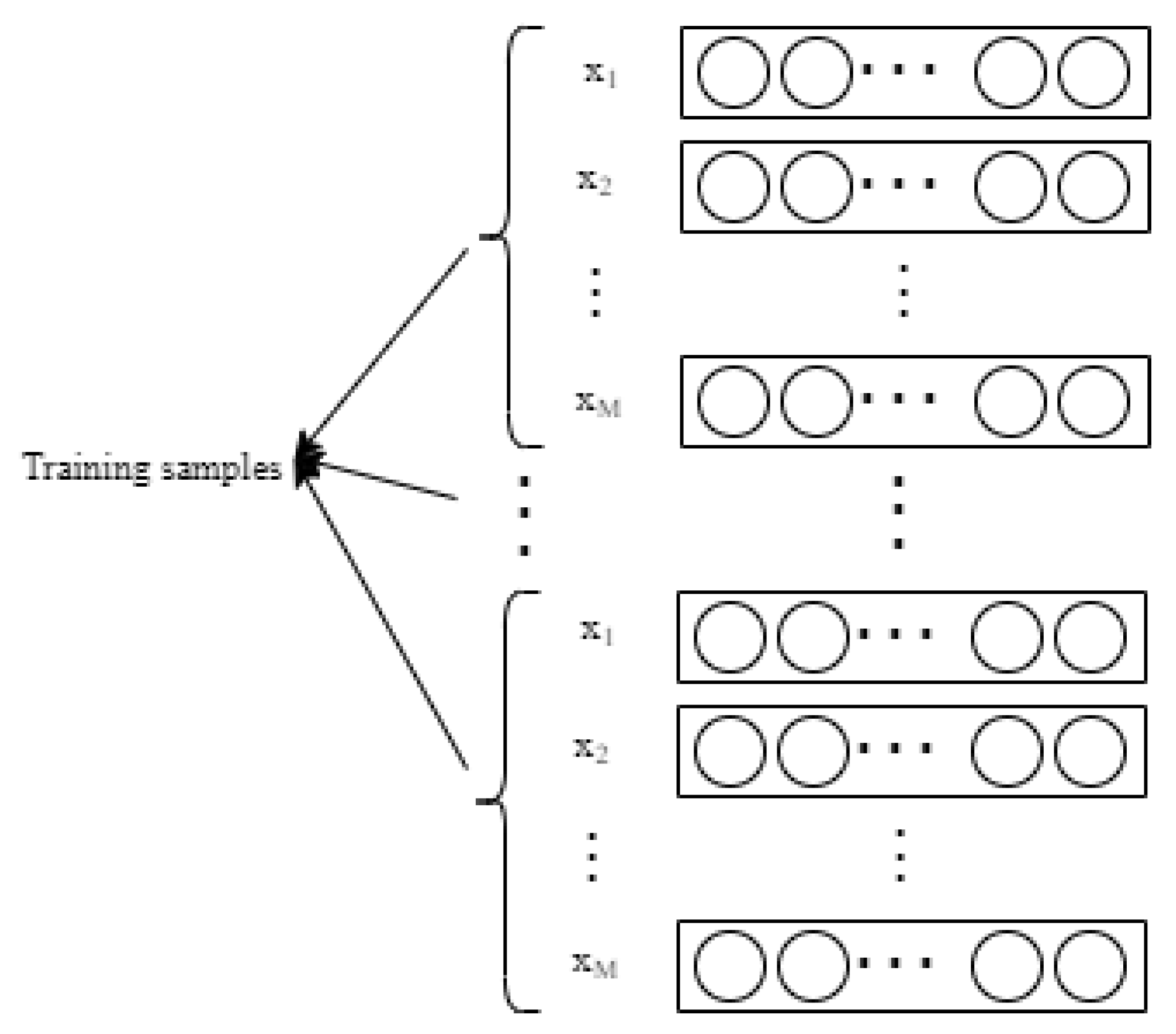
In LSANPD, we propose a combination of LSTM and self-attention using stacked LSTM layers and multi-head self-attention sub-block, as shown in Figure 7b. Input sequence $\left\{{\mathbf{x}}_1,{\mathbf{x}}_2,...,{\mathbf{x}}_M\right\}$ in (1) is fed into the LSTM block, and $\left\{{\tilde{\mathbf{x}}}_1,{\tilde{\mathbf{x}}}_2,...,{\tilde{\mathbf{x}}}_M\right\}$ can be obtained using the LSTM mechanism, as shown in Figure 10. Then, all vector outputs are linked together to form the $\tilde{\mathbf{X}}=\left[{{\tilde{\mathbf{x}}}_1}^T,{{\tilde{\mathbf{x}}}_2}^T,\cdots ,{{\tilde{\mathbf{x}}}_M}^T\right]$ matrix as the SAB input. The next steps are performed on the SAB and classification block, similar to those in the SANPD model.

3.3. Training

The SANPD and LSANPD parameters are learned through training dataset L to minimize the loss function in the classification block. The parameter set includes hyper parameters, weight parameters, and bias parameters. In the proposed SANPD and LSANPD, the cross-entropy loss function is used. Thus, the loss function of the lth training data is formulated as follows:

$$Loss({\mathbf{v}}^{\left(l\right)},z^{\left(l\right)})=-log\left(z^{\left(l\right)}\right),$$

(13)

where ${\mathbf{v}}^{\left(l\right)}={\left[v_1,\dots ,v_C\right]}^T$ is the label that corresponds to the lth training data in which $v_i=1$ if the true classification is fault type i. The other cases are $v_c=0$ for $c\ne i$, and $z^{\left(l\right)}=z_i$ if the predicted classification of the lth training data is a type-i fault. The target of the training process is to find the suitable parameters that minimize the cost function of the entry training dataset:

$$I\left(\mathsf{\Theta }\right)=\frac{1}{\left|L\right|}\sum _{l\in L}Loss({\mathbf{v}}^{\left(l\right)},z^{\left(l\right)}),$$

(14)

where $\mathsf{\Theta }$ represents all learnable parameters and $\left|·\right|$ is the number of elements in a set.

To minimize the loss function, many variants of the gradient-descent method have been studied in the literature, such as AdaGrad, AdaDelta, Adam, and Nestrove momentum, into the ADAM optimizer [57,58,59,60]. These optimizers adaptively change the learning rate to properly minimize the loss function. We select the Nestrove momentum in the ADAM optimizer in our experiments.

4. Performance Evaluation

This section presents a performance analysis of the proposed models using PRPD data from PD experiments and noise measurements. The performance of the proposed models is compared to that of the recently developed RNN model [46], which has achieved significant performance improvement over existing machine-learning methods and other techniques. For comparison purposes, we consider this model as the baseline system.

For PRPD experiments, four types of faults, such as corona, floating, particle, and void faults are considered.

Table 1. Experimental dataset.

Fault Types	Corona	Floating	Particle	Void	Noise
Number of experiments	94	35	66	242	298

shows the numbers of experiments for each fault type and noise, where one experiment for PRPD and noise measurements includes 3600 power cycles and the total number of experiments is defined as $K=735$.

Figure 11 shows the data-augmentation process. The data that have been used in this study include $K=735$ experiments of PRPD faults. Each experiment is performed at 3600 power cycles. To overcome the issue of overfitting during the training process, we applied a data-argumentation technique to increase the number of training samples [61]. We divided every experiment into $M=60$ equally small groups containing 60 power cycles (3600 in total). Afterward, the total number of data samples became $KM=$ 44,100.

We split the dataset into three parts: training, validation, and test sets. We used 81%, 9%, and 10% of the data for these three sets, respectively. Thus, we have a total of 35,721 training, 3969 validation, and 4410 test samples.

Multiple experiments with different numbers of attention heads and SABs were conducted using the validation data. With different parameters to tune our model, extensive experiments were conducted to obtain the other optimized hyperparameters such as the batch size, number of epochs, and learning rate. The model parameters for the proposed architectures are listed in

Table 2. Details of proposed SANPD.

Layer Name	Output Dimension	Activation Function	Numberof Parameters
Input Layer	$60\times 128$	-	0
i-th Self-attention	$60\times 16$	-	6144
$\left(i\in \left\{1,...,8\right\}\right)$
Concatenate	$60\times 128$	-	0
Add	$60\times 128$	-	0
Dense Layer 1	$60\times 128$	ReLU	16,512
Dense Layer 2	$60\times 128$	-	16,512
Add	$60\times 128$	-	0
Max pooling	$1\times 128$	-	0
Dense Layer 3	$1\times 64$	ReLU	8256
Dense Layer 4	$1\times 5$	Softmax	325

and

Table 3. Details of proposed LSANPD.

Layer Name	Output Dimension	Activation Function	Numberof Parameters
Input Layer	$60\times 128$	-	0
LSTM	$60\times 128$	-	131,584
i-th Self-attention	$60\times 16$	-	6144
$\left(i\in \left\{1,...,8\right\}\right)$
Concatenate	$60\times 128$	-	0
Add	$60\times 128$	-	0
Dense Layer 1	$60\times 128$	ReLU	16,512
Dense Layer 2	$60\times 128$	-	16,512
Add	$60\times 128$	-	0
Max pooling	$1\times 128$	-	0
Dense Layer 3	$1\times 64$	ReLU	8256
Dense Layer 4	$1\times 5$	Softmax	325

, where the output shapes, activation functions, and numbers of trainable parameters are presented. During our experiments, we performed 20 trials to mitigate the effects of random initialization of the neural network and then the results were averaged to confirm the robustness of our proposed model. During the training process, the optimization step was carried out according to small batches of 512 samples, and the learning rate was 0.001. The model was implemented using Keras [62] with TensorFlow [63], which is a deep learning framework of Google.

The list in

Table 4. Performance comparisons in terms of accuracy.

Fault Types	Overall	Corona	Floating	Particle	Void	Noise
LSTM RNN [46]	92.5	94.8	80.0	69.9	96.7	94.5
SANPD	93.8	95.0	81.4	85.5	96.7	94.2
LSANPD	94.0	95.4	81.9	81.8	97.7	94.5

illustrates the comparison between the SANPD, LSANPD, and LSTM RNN methods in [46]. The overall accuracy and classification accuracy in each fault of the SANPD and LSANPD outperform that of the RNN because the SABs are able to capture the relevance among the PRPD phases by considering their entire interaction sequence input regardless of the distance. Moreover, the LSANPD improves the performance compared to the LSTM RNN owing to the self-attention mechanism that assists the LSTM in simultaneously computing and focusing on the important information of the sequence input, where the accuracy of the LSTM RNN is quite high compared with traditional methods such as the linear SVM and artificial neural network (Table 2 [46]). In addition, the performance of the proposed SANPD and LSANPD is comparably obtained. Performance accuracy for each fault is also presented in Table 4. It can be observed that most models (for corona, void, and noise data) managed to perform efficiently. Furthermore, it was difficult to classify floating and partial faults because the amount of data of the floating and partial faults was smaller than that of the other faults, as shown in Table 1.

Table 5. Comparison of complexity.

Model	Numberof Parameters	Training Time $\left(\mathit{s}\right)$	Test Time $\left(\mathit{s}\right)$
LSTM RNN [46]	264 k	667	217
SANPD	90 k	420	210
LSANPD	222 k	974	284

lists the comparison of the models in terms of the number of parameters and computation training and test times. SANPD demonstrates the lowest number of parameters of approximately 90,000, whereas the number of LSTM RNN parameters is approximately 264,000, which is 2.9 times larger. The parameters of the LSANPD method is approximately 222,000, which is 1.2 times lower than that of the LSTM RNN. The training and test times of SANPD are faster than those of RNN by approximately 1.8 and 1.03 times, respectively. They are respectively 2.3 and 1.3 times lower than those of LSANPD. In terms of complexity, SANPD is better than LSANPD and LSTM RNN because SANPD has a self-attention mechanism parallel architecture without a recurrent or convolution module in the PRPD phase while LSANPD has an LSTM structure, which increases the model complexity.

In terms of accuracy performance, the proposed SANPD and LSANPD are superior to the existing LSTM RNN model [46]. Although SANPD exhibits slightly lower accuracy performance than LSANPD by 0.2 times, it is significantly better than the LSANPD and LSTM RNN in terms of complexity.

5. Conclusions

Deep learning is a fast-evolving technique that has many implications in many different applications. However, the performance of the existing deep learning approaches is not further improved for the sequential PRPD data because the models are not capable of simultaneous computation and learning the important relevance of inputs. To deal with the problems, a state-of-the-art self-attention-based neural-network technique is investigated to classify faults in the GIS. In the proposed model, the multi-head self-attention is implemented to learn the interactions of the PD signals by focusing on the important information of the PRPD sequence input and improve computation and performance using parallelism. The experimental results show that the SANPD outperforms the previous LSTM RNN model in terms of accuracy and complexity. SANPD has slightly lower accuracy than LSANPD. However, it reduces the complexity compared with LSANPD because it takes advantage of parallel computation. Therefore, the proposed method can be successfully applied to fault diagnosis in GISs.

For future work, we will install the PD diagnosis systems in power grids. The proposed scheme will be further verified to improve the robustness at various noise conditions (depending on time, location, GIS, and antenna design) and detect various faults using experimental data, including corona discharges, floating discharges, particle discharges, and void discharges at three/four different levels of voltage.

References

1. Bolin, P.; Koch, H. Gas insulated substation GIS. In Proceedings of the IEEE/PES Transmission and Distribution Conference and Exposition, Chicago, IL, USA, 21–24 April 2008; pp. 1–3. [Google Scholar] [CrossRef]
2. Tang, J.; Zhuo, R.; Wang, D.; Wu, J.; Zhang, X. Application of SA-SVM Incremental Algorithm in GIS PD Pattern Recognition. J. Electr. Eng. Technol. 2016, 11, 192–199. [Google Scholar] [CrossRef] [Green Version]
3. Lee, S.; Lee, B.; Koo, J.; Ryu, C.; Jung, S. Identification of insulation defects in gas-insulated switchgear by chaotic analysis of partial discharge. IET Sci. Meas. Technol. 2010, 4, 115–124. [Google Scholar] [CrossRef]
4. Gao, W.; Ding, D.; Liu, W. Research on the Typical Partial Discharge Using the UHF Detection Method for GIS. IEEE Trans. Power Deliv. 2011, 26, 2621–2629. [Google Scholar] [CrossRef]
5. Stone, G. Partial discharge diagnostics and electrical equipment insulation condition assessment. IEEE Trans. Dielectr. Electr. Insul. 2005, 12, 891–903. [Google Scholar] [CrossRef]
6. Wu, M.; Cao, H.; Cao, J.; Nguyen, H.L.; Gomes, J.B.; Krishnaswamy, S.P. An overview of state-of-the-art partial discharge analysis techniques for condition monitoring. IEEE Electr. Insul. Mag. 2015, 31, 22–35. [Google Scholar] [CrossRef]
7. Dong, M.; Zhang, C.; Ren, M.; Albarracín, R.; Ye, R. Electrochemical and Infrared Absorption Spectroscopy Detection of SF6 Decomposition Products. Sensors 2017, 17, 2627. [Google Scholar] [CrossRef] [Green Version]
8. Judd, M.; Li, Y.; Hunter, I. Partial discharge monitoring of power transformers using UHF sensors. Part I: Sensors and signal interpretation. IEEE Electr. Insul. Mag. 2005, 21, 5–14. [Google Scholar] [CrossRef]
9. Judd, M.; Farish, O.; Hampton, B. The excitation of UHF signals by partial discharges in GIS. IEEE Trans. Dielectr. Electr. Insul. 1996, 3, 213–228. [Google Scholar] [CrossRef]
10. Cosgrave, J.; Vourdas, A.; Jones, G.; Spencer, J.; Murphy, M.; Wilson, A. Acoustic monitoring of partial discharges in gas insulated substations using optical sensors. IEE Proc. A Sci. Meas. Technol. UK 1993, 140, 369. [Google Scholar] [CrossRef]
11. Markalous, S.; Tenbohlen, S.; Feser, K. Detection and location of partial discharges in power transformers using acoustic and electromagnetic signals. IEEE Trans. Dielectr. Electr. Insul. 2008, 15, 1576–1583. [Google Scholar] [CrossRef]
12. Imad-U-Khan; Wang, Z.; Cotton, I.; Northcote, S. Dissolved gas analysis of alternative fluids for power transformers. IEEE Electr. Insul. Mag. 2007, 23, 5–14. [Google Scholar] [CrossRef]
13. Faiz, J.; Soleimani, M. Dissolved gas analysis evaluation in electric power transformers using conventional methods a review. IEEE Trans. Dielectr. Electr. Insul. 2017, 24, 1239–1248. [Google Scholar] [CrossRef]
14. Chai, H.; Phung, B.; Mitchell, S. Application of UHF Sensors in Power System Equipment for Partial Discharge Detection: A Review. Sensors 2019, 19, 1029. [Google Scholar] [CrossRef] [PubMed] [Green Version]
15. Siegel, M.; Coenen, S.; Beltle, M.; Tenbohlen, S.; Weber, M.; Fehlmann, P.; Hoek, S.M.; Kempf, U.; Schwarz, R.; Linn, T.; et al. Calibration Proposal for UHF Partial Discharge Measurements at Power Transformers. Energies 2019, 12, 3058. [Google Scholar] [CrossRef] [Green Version]
16. Piccin, R.; Mor, A.; Morshuis, P.; Girodet, A.; Smit, J. Partial discharge analysis of gas insulated systems at high voltage AC and DC. IEEE Trans. Dielectr. Electr. Insul. 2015, 22, 218–228. [Google Scholar] [CrossRef]
17. Dai, D.; Wang, X.; Long, J.; Tian, M.; Zhu, G.; Zhang, J. Feature extraction of GIS partial discharge signal based on S-transform and singular value decomposition. IET Sci. Meas. Technol. 2017, 11, 186–193. [Google Scholar] [CrossRef]
18. Si, W.; Li, J.; Li, D.; Yang, J.; Li, Y. Investigation of a comprehensive identification method used in acoustic detection system for GIS. IEEE Trans. Dielectr. Electr. Insul. 2010, 17, 721–732. [Google Scholar] [CrossRef]
19. Chang, C.; Jin, J.; Chang, C.; Hoshino, T.; Hanai, M.; Kobayashi, N. Separation of Corona Using Wavelet Packet Transform and Neural Network for Detection of Partial Discharge in Gas-Insulated Substations. IEEE Trans. Power Deliv. 2005, 20, 1363–1369. [Google Scholar] [CrossRef]
20. Zhang, X.; Xiao, S.; Shu, N.; Tang, J.; Li, W. GIS partial discharge pattern recognition based on the chaos theory. IEEE Trans. Dielectr. Electr. Insul. 2014, 21, 783–790. [Google Scholar] [CrossRef]
21. Li, L.; Tang, J.; Liu, Y. Partial discharge recognition in gas insulated switchgear based on multi-information fusion. IEEE Trans. Dielectr. Electr. Insul. 2015, 22, 1080–1087. [Google Scholar] [CrossRef]
22. Liu, X.W.; Mu, H.B.; Zhu, M.X.; Zhang, G.J.; Li, Y.; Deng, J.B.; Xue, J.Y.; Shao, X.J.; Zhang, J.N. Classification and separation of partial discharge ultra-high-frequency signals in a 252 kV gas insulated substation by using cumulative energy technique. IET Sci. Meas. Technol. 2016, 10, 316–326. [Google Scholar] [CrossRef]
23. Gao, W.; Zhao, D.; Ding, D.; Yao, S.; Zhao, Y.; Liu, W. Investigation of frequency characteristics of typical PD and the propagation properties in GIS. IEEE Trans. Dielectr. Electr. Insul. 2015, 22, 1654–1662. [Google Scholar] [CrossRef]
24. Mas’ud, A.A.; Ardila-Rey, J.A.; Albarracín, R.; Muhammad-Sukki, F.; Bani, N.A. Comparison of the Performance of Artificial Neural Networks and Fuzzy Logic for Recognizing Different Partial Discharge Sources. Energies 2017, 10, 1060. [Google Scholar] [CrossRef] [Green Version]
25. Adam, B.; Tenbohlen, S. Classification of multiple PD Sources by Signal Features and LSTM Networks. In Proceedings of the IEEE International Conference on High Voltage Engineering and Application (ICHVE), Athens, Greece, 10–13 September 2018; pp. 1–4. [Google Scholar] [CrossRef]
26. Yan, Z.; Min-Jie, Z.; Peng, Y.; Yan-Ming, L. Study on pulse source separation and location technology of UHF PD based on three-dimensional vector of pulse amplitude in time domain. In Proceedings of the IEEE International Conference on High Voltage Engineering and Application (ICHVE), Chengdu, China, 19–22 September 2018; pp. 1–4. [Google Scholar] [CrossRef]
27. Nair, R.P.; Vishwanath, S.B. Analysis of partial discharge sources in stator insulation system using variable excitation frequency. IET Sci. Meas. Technol. 2019, 13, 922–930. [Google Scholar] [CrossRef]
28. Banumathi, S.; Chandrasekar, S.; Montanari, G.C. Investigations on PD characteristics of vegetable oils for high voltage applications. In Proceedings of the IEEE 1st International Conference on Condition Assessment Techniques in Electrical Systems (CATCON), Kolkata, India, 6–8 December 2013; pp. 191–195. [Google Scholar] [CrossRef]
29. Kunicki, M.; Nagi, L. Correlation analysis of partial discharge measurement results. In Proceedings of the IEEE International Conference on Environment and Electrical Engineering and 2017 IEEE Industrial and Commercial Power Systems Europe (EEEIC/I&CPS Europe), Milan, Italy, 6–9 June 2017; pp. 1–6. [Google Scholar] [CrossRef]
30. Yang, J.; Zhang, D.; Frangi, A.; Yang, J.-Y. Two-dimensional pca: A new approach to appearance-based face representation and recognition. IEEE Trans. Pattern Anal. Mach. Intell. 2004, 26, 131–137. [Google Scholar] [CrossRef] [Green Version]
31. Yan, W.; Goebel, K.F. Feature dimensionality reduction for partial discharge diagnoise of aircraft wiring. In Proceedings of the 59th Meeting of the Society for Machine Failure Prevention Technology, MFPT ’05, Virginia Beach, VA, USA, 18–21 April 2005; pp. 167–176. [Google Scholar]
32. Lai, K.; Phung, B.; Blackburn, T. Partial Discharge Analysis using PCA and SOM. In Proceedings of the IEEE Lausanne Power Tech, Lausanne, Switzerland, 1–5 July 2007; pp. 2133–2138. [Google Scholar] [CrossRef]
33. Ma, H.; Chan, J.C.; Saha, T.K.; Ekanayake, C. Pattern recognition techniques and their applications for automatic classification of artificial partial discharge sources. IEEE Trans. Dielectr. Electr. Insul. 2013, 20, 468–478. [Google Scholar] [CrossRef] [Green Version]
34. Abdel-Galil, T.; Sharkawy, R.; Salama, M.; Bartnikas, R. Partial Discharge Pattern Classification Using the Fuzzy Decision Tree Approach. IEEE Trans. Instrum. Meas. 2005, 54, 2258–2263. [Google Scholar] [CrossRef]
35. Hao, L.; Lewin, P. Partial discharge source discrimination using a support vector machine. IEEE Trans. Dielectr. Electr. Insul. 2010, 17, 189–197. [Google Scholar] [CrossRef]
36. Schmidhuber, J. Deep Learning in Neural Networks: An Overview. Neural Net. 2015, 61, 85–117. [Google Scholar] [CrossRef] [Green Version]
37. Duan, L.; Hu, J.; Zhao, G.; Chen, K.; He, J.; Wang, S.X. Identification of Partial Discharge Defects Based on Deep Learning Method. IEEE Trans. Power Deliv. 2019, 34, 1557–1568. [Google Scholar] [CrossRef]
38. Campos, V.; Jou, B.; Giró-i Nieto, X. From pixels to sentiment: Fine-tuning CNNs for visual sentiment prediction. Elsevier 2017, 65, 15–22. [Google Scholar] [CrossRef] [Green Version]
39. Brocki, L.; Marasek, K. Deep Belief Neural Networks and Bidirectional Long-Short Term Memory Hybrid for Speech Recognition. Arch. Acoust. 2015, 40, 191–195. [Google Scholar] [CrossRef] [Green Version]
40. Tai, K.S.; Socher, R.; Manning, C.D. Improved Semantic Representations From Tree-Structured Long Short-Term Memory Networks. In Proceedings of the 53rd Annual Meeting of the Association for Computational Linguistics and the 7th International Joint Conference on Natural Language Processing (Volume 1: Long Papers), Beijing, China, 26–31 July 2015; pp. 1556–1566. [Google Scholar] [CrossRef] [Green Version]
41. Catterson, V.M.; Sheng, B. Deep neural networks for understanding and diagnosing partial discharge data. In Proceedings of the IEEE Electrical Insulation Conference (EIC), Seattle, WA, USA, 7–10 June 2015; pp. 218–221. [Google Scholar] [CrossRef] [Green Version]
42. Song, H.; Dai, J.; Sheng, G.; Jiang, X. GIS partial discharge pattern recognition via deep convolutional neural network under complex data source. IEEE Trans. Dielectr. Electr. Insul. 2018, 25, 678–685. [Google Scholar] [CrossRef]
43. Liu, G.; Guo, J. Bidirectional LSTM with attention mechanism and convolutional layer for text classification. Neurocomputing 2019, 337, 325–338. [Google Scholar] [CrossRef]
44. Sun, S.; Tang, Y.; Dai, Z.; Zhou, F. Self-Attention Network for Session-Based Recommendation With Streaming Data Input. IEEE Access 2019, 7, 110499–110509. [Google Scholar] [CrossRef]
45. Vaswani, A.; Shazeer, N.; Parmar, N.; Uszkoreit, J.; Jones, L.; Gomez, A.N.; Kaiser, L.; Polosukhin, I. Attention Is All You Need. In Advances in Neural Information Processing Systems; MIT Press: Long Beach, CA, USA, 2017; pp. 5998–6008. [Google Scholar]
46. Nguyen, M.T.; Nguyen, V.H.; Yun, S.J.; Kim, Y.H. Recurrent Neural Network for Partial Discharge Diagnosis in Gas-Insulated Switchgear. Energies 2018, 11, 1202. [Google Scholar] [CrossRef] [Green Version]
47. Gao, W.; Ding, D.; Liu, W.; Huang, X. Investigation of the Evaluation of the PD Severity and Verification of the Sensitivity of Partial-Discharge Detection Using the UHF Method in GIS. IEEE Trans. Power Deliv. 2014, 29, 38–47. [Google Scholar] [CrossRef]
48. Young, T.; Hazarika, D.; Poria, S.; Cambria, E. Recent Trends in Deep Learning Based Natural Language Processing [Review Article]. IEEE Comput. Intell. Mag. 2018, 13, 55–75. [Google Scholar] [CrossRef]
49. Bai, T.; Nie, J.Y.; Zhao, W.X.; Zhu, Y.; Du, P.; Wen, J.R. An Attribute-aware Neural Attentive Model for Next Basket Recommendation. In Proceedings of the 41st International ACM SIGIR Conference on Research & Development in Information Retrieval—SIGIR ’18, Ann Arbor, MI, USA, 8–12 July 2018; pp. 1201–1204. [Google Scholar] [CrossRef]
50. Zheng, L.; Lu, C.T.; He, L.; Xie, S.; He, H.; Li, C.; Noroozi, V.; Dong, B.; Yu, P.S. MARS: Memory Attention-Aware Recommender System. In Proceedings of the IEEE International Conference on Data Science and Advanced Analytics (DSAA), Washington, DC, USA, 5–8 October 2019; pp. 11–20. [Google Scholar] [CrossRef] [Green Version]
51. Bahdanau, D.; Cho, K.; Bengio, Y. Neural Machine Translation by Jointly Learning to Align and Translate. In Proceedings of the 3rd International Conference on Learning Representations (ICLR 2015), San Diego, CA, USA, 7–9 May 2015. [Google Scholar]
52. Luong, T.; Pham, H.; Manning, C.D. Effective Approaches to Attention-based Neural Machine Translation. In Proceedings of the 2015 Conference on Empirical Methods in Natural Language Processing, Lisbon, Portugal, 17–21 September 2015; pp. 1412–1421. [Google Scholar] [CrossRef] [Green Version]
53. He, K.; Zhang, X.; Ren, S.; Sun, J. Deep Residual Learning for Image Recognition. In Proceedings of the IEEE Conference on Computer Vision and Pattern Recognition (CVPR), Las Vegas, NV, USA, 27–30 June 2016; pp. 770–778. [Google Scholar] [CrossRef] [Green Version]
54. Nair, V.; Hinton, G.E. Rectified Linear Units Improve Restricted Boltzmann Machines. In Proceedings of the 27th International Conference on International Conference on Machine Learning (ICML’10), Haifa, Israel, 21–24 June 2010; Volume 27, pp. 807–814. [Google Scholar]
55. Anastasopoulos, A.; Chiang, D. Tied Multitask Learning for Neural Speech Translation. In Proceedings of the 2018 Conference of the North American Chapter of the Association for Computational Linguistics: Human Language Technologies, Volume 1 (Long Papers), New Orleans, Louisiana, 1–6 June 2018; pp. 82–91. [Google Scholar] [CrossRef] [Green Version]
56. Nwankpa, C.; Ijomah, W.; Gachagan, A.; Marshall, S. Activation Functions: Comparison of trends in Practice and Research for Deep Learning. Cornell Univ. 2018, 20, 1–20. [Google Scholar]
57. Duchi, J.; Hazan, E.; Singer, Y. Adaptive Subgradient Methods for Online Learning and Stochastic Optimization. J. Mach. Learn. Res. 2011, 12, 2121–2159. [Google Scholar]
58. Zeiler, M.D. ADADELTA: An Adaptive Learning Rate Method. arXiv 2012, arXiv:1212.5701. [Google Scholar]
59. Kingma, D.P.; Ba, J. Adam: A Method for Stochastic Optimization. In Proceedings of the 3rd International Conference for Learning Representations, San Diego, CA, USA, 7–9 May 2015; pp. 807–814. [Google Scholar]
60. Dozat, T. Incorporating Nesterov Momentum into Adam. In Proceedings of the ICLR Workshop, Caribe Hilton, San Juan, Puerto Rico, 2–4 May 2016; pp. 2013–2016. [Google Scholar]
61. Cui, X.; Goel, V.; Kingsbury, B. Data augmentation for deep convolutional neural network acoustic modeling. In Proceedings of the IEEE International Conference on Acoustics, Speech and Signal Processing (ICASSP), South Brisbane, Queensland, Australia, 19–24 September 2015; pp. 4545–4549. [Google Scholar] [CrossRef]
62. Keras-team.2015. Available online: https://github.com/fchollet/keras (accessed on 22 October 2017).
63. Abadi, M.; Agarwal, A.; Barham, P.; Brevdo, E.; Chen, Z.; Citro, C.; Corrado, G.; Davis, A.; Dean, J.; Devin, M. TensorFlow: Large-Scale Machine Learning on Heterogeneous Distributed Systems. 2015. Available online: https://www.tensorflow.org/ (accessed on 3 April 2020).
Figure 1. Artificial cells for the simulated (a) corona, (b) floating, (c) void, and (d) particle partial discharges (PDs).
Energies 13 02102 g001
Figure 2. Phase-resolved PD (PRPD) fault types in the GIS: (a) corona, (b) floating, (c) void, and (d) particle faults.
Energies 13 02102 g002
Figure 3. Two-dimensional representation of PRPDs in the gas-insulated switchgear (GIS): (a) corona, (b) floating, (c) void, and (d) particle faults.
Energies 13 02102 g003
Figure 4. (a) A block diagram of PD measurement and (b) installation of ultra-high-frequency (UHF) sensors.
Energies 13 02102 g004
Figure 5. Measured reflection coefficient of the external UHF sensor.
Energies 13 02102 g005
Figure 6. Example of noise in on-site measurements.
Energies 13 02102 g006
Figure 7. Architecture of the proposed methods. (a) Self-attention-based neural network for PRPDs (SANPD). (b) Long short-term memory SANPD (LSANPD).
Energies 13 02102 g007
Figure 8. Self-attention blocks (SAB) architecture.
Energies 13 02102 g008
Figure 9. Architecture of the classification block.
Energies 13 02102 g009
Figure 10. LSTM block architecture.
Energies 13 02102 g010
Figure 11. Data augmentation of the PRPD data.
Energies 13 02102 g011